Sparse Bayesian Learning and the Relevance Vector Machine

Michael E. Tipping

article2001JMLR2,640 citations

Introduces the Relevance Vector Machine, a sparse Bayesian learning framework that matches the generalization accuracy of support vector machines while producing dramatically sparser models, delivering calibrated probabilistic predictions, and automatically estimating hyperparameters without cross-validation.

Listen

Supervised learning tasks such as regression and classification frequently encounter overfitting when models use as many parameters as training examples. Support vector machines address this through margin maximization but require cross-validation for key parameters, produce non-probabilistic outputs, and restrict kernels to those satisfying Mercer's condition. These constraints limit practical deployment where uncertainty estimates or computational efficiency matter.

The article presents a fully Bayesian alternative called the relevance vector machine. It places a hierarchical prior on model weights, with one hyperparameter per weight, and estimates those hyperparameters by maximizing the marginal likelihood of the data. This procedure automatically prunes most weights to zero while delivering predictions and, in regression, error bars. The same framework applies to both regression and classification without requiring separate tuning steps.

Experiments on synthetic functions and standard benchmarks show that relevance vector machines match or exceed support vector machine accuracy while using far fewer basis functions, typically 10 to 20 percent as many. The models also supply well-calibrated posterior probabilities in classification and allow arbitrary basis functions, including direct optimization of input scale parameters within the kernel. These advantages arise because the Bayesian treatment concentrates posterior mass on sparse solutions.

The resulting sparsity reduces memory and prediction cost, while probabilistic outputs enable proper handling of asymmetric losses and class imbalance. Automatic parameter estimation removes the need for cross-validation, simplifying model deployment. For very large training sets the original algorithm scales as the cube of the number of examples, though a constructive variant mitigates this.

Practitioners should evaluate the relevance vector machine when sparse probabilistic models are needed and data volume permits the cubic training cost. Additional work on scaling and on criteria for kernel selection would further broaden applicability. Results rest on consistent performance across repeated trials and multiple data sets, with the main uncertainty lying in behavior on extremely large problems where only the improved algorithm has been tested.

Microsoft bayesian learning bayesian methods classification methods Relevance Vector Machine Sparse Bayesian Learning Support Vector Machine

Tipping (2001).pdf

Paper: Support Vector Regression Machines, Harris Drucker et al. (1996). Introduces support vector regression using insensitive loss functions and margin regularization, providing the primary non-probabilistic benchmark that the Relevance Vector Machine seeks to reformulate and improve upon.
Paper: Support-vector networks, Corinna Cortes et al. (1995). Establishes the foundational support-vector network architecture for classification, defining the standard margin-maximization and kernel framework that the source replaces with a sparse Bayesian formulation.
Paper: A training algorithm for optimal margin classifiers, B. Boser et al. (1992). Presents the original optimal margin classifier and dual formulation that motivate the source's pursuit of sparsity and kernel-based pattern recognition.
Paper: Support Vector Method for Function Approximation, Regression Estimation and Signal Processing, V. Vapnik et al. (1996). Extends support vector machines to high-dimensional function approximation and regression, establishing key baseline concepts for sparse kernel estimation.
Paper: Keeping Neural Networks Simple by Minimizing the Description Length of the Weights, Geoffrey E. Hinton et al. (1993). Demonstrates how placing adaptive Gaussian priors on parameters penalizes model complexity, foreshadowing the hierarchical prior framework utilized in sparse Bayesian learning.

Paper: Choosing Multiple Parameters for Support Vector Machines, OLIVIER CHAPELLE et al. (2002). Extends hyperparameter optimization in kernel methods by computing gradients of generalization bounds to tune feature scaling parameters, paralleling the source's capacity for automated parameter selection.
Paper: Learning the Kernel Matrix with Semidefinite Programming, Gert R. G. Lanckriet et al. (2004). Develops semidefinite programming techniques to automatically optimize kernel matrices directly from data, providing an alternative non-Bayesian solution to the kernel selection challenge highlighted in the source.
Paper: Feature selection, L1 vs. L2 regularization, and rotational invariance, A. Ng (2004). Provides a theoretical comparison of sparsity-inducing L1 regularization versus L2 regularization under high dimensions, enriching the conceptual understanding of sparse learning mechanisms.
Paper: An Introduction to Variable and Feature Selection, Isabelle M Guyon et al. (2003). Surveys systematic variable and feature selection techniques, framing the sparse parameter pruning achieved by the Relevance Vector Machine within the broader landscape of model selection.
Paper: On Over-fitting in Model Selection and Subsequent Selection Bias in Performance Evaluation, G. Cawley et al. (2010). Analyzes the risk of overfitting during hyperparameter selection in kernel machines and Gaussian processes, critically evaluating the automated model selection properties discussed in the source.
Paper: Random Features for Large-Scale Kernel Machines, Ali Rahimi et al. (2007). Introduces explicit random feature mappings to overcome cubic kernel scaling bottlenecks, directly addressing the computational scaling challenges associated with kernel and relevance vector methods.
Paper: An empirical comparison of supervised learning algorithms, R. Caruana et al. (2006). Benchmarks probability calibration across diverse learning algorithms, validating the practical significance of the well-calibrated posterior probabilities generated by Bayesian kernel approaches.

Cover for Sparse Bayesian Learning and the Relevance Vector Machine

Abstract

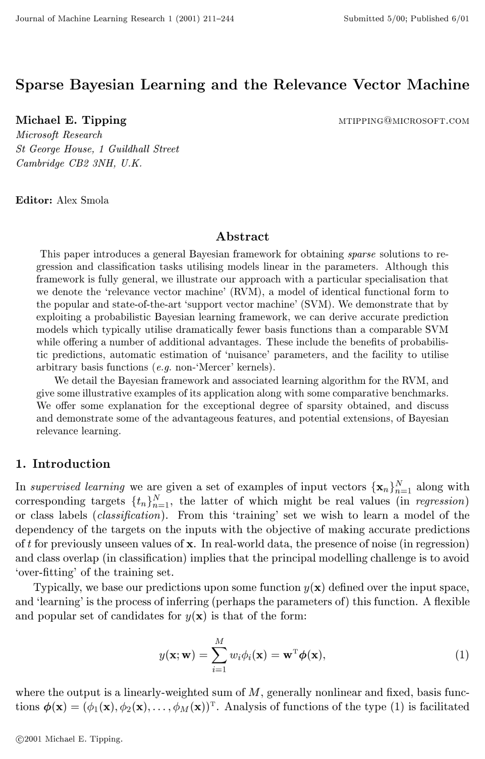
This paper introduces a general Bayesian framework for obtaining sparse solutions to regression and classification tasks utilising models linear in the parameters. Although this framework is fully general, we illustrate our approach with a particular specialisation that we denote the ‘relevance vector machine’ (RVM), a model of identical functional form to the popular and state-of-the-art ‘support vector machine’ (SVM). We demonstrate that by exploiting a probabilistic Bayesian learning framework, we can derive accurate prediction models which typically utilise dramatically fewer basis functions than a comparable SVM while offering a number of additional advantages. These include the benefits of probabilistic predictions, automatic estimation of ‘nuisance’ parameters, and the facility to utilise arbitrary basis functions (e.g. non-Mercer’ kernels).

We detail the Bayesian framework and associated learning algorithm for the RVM, and give some illustrative examples of its application along with some comparative benchmarks. We offer some explanation for the exceptional degree of sparsity obtained, and discuss and demonstrate some of the advantageous features, and potential extensions, of Bayesian relevance learning.

BDBA D2D8D6D3CSD9CRD8CXD3D2
BEBA CBD4CPD6D7CT BUCPDDCTD7CXCPD2 CTCPD6D2CXD2CV CUD3D6 CACTCVD6CTD7D7CXD3D2
BEBABD D3CSCTD0 CBD4CTCRCXACCRCPD8CXD3D2
BEBABE D2CUCTD6CTD2CRCT
BEBABF D4D8CXD1CXD7CXD2CV D8CWCT DDD4CTD6D4CPD6CPD1CTD8CTD6D7
BEBABG CPCZCXD2CV D6CTCSCXCRD8CXD3D2D7
BFBA CBD4CPD6D7CT BUCPDDCTD7CXCPD2 BVD0CPD7D7CXACCRCPD8CXD3D2
BGBA CACTD0CTDACPD2CRCT CECTCRD8D3D6 BXDCCPD1D4D0CTD7
BGBABD CACTD0CTDACPD2CRCT CECTCRD8D3D6 CACTCVD6CTD7D7CXD3D2BM D8CWCT COD7CXD2CRB3 CUD9D2CRD8CXD3D2
BGBABE CACTD0CTDACPD2CRCT CECTCRD8D3D6 BVD0CPD7D7CXACCRCPD8CXD3D2BM CACXD4D0CTDDB3D7 D7DDD2D8CWCTD8CXCR CSCPD8CP
BGBABF BXDCD8CTD2D7CXD3D2D7
BGBABG BUCTD2CRCWD1CPD6CZ BVD3D1D4CPD6CXD7D3D2D7
BGBABGBABD CACTCVD6CTD7D7CXD3D2
BGBABGBABE BVD0CPD7D7CXCUCXCRCPD8CXD3D2
BHBA CTD6D7D4CTCRD8CXDACTD7 D3D2 CBD4CPD6D7CXD8DD
BHBABD CCCWCT D6CXD3D6 D3DACTD6 D8CWCT CFCTCXCVCWD8D7
BHBABE BT BZCPD9D7D7CXCPD2 D6D3CRCTD7D7 CECXCTDB
BIBA BWCXD7CRD9D7D7CXD3D2
BTCRCZD2D3DBD0CTCSCVD1CTD2D8D7
BTD4D4CTD2CSCXDC BTBA BYD9D6D8CWCTD6 BWCTD8CPCXD0D7 D3CU CACTD0CTDACPD2CRCT CECTCRD8D3D6 CTCPD6D2CXD2CV
BTBABD BVD3D1D4D9D8CXD2CV D8CWCT D3CV CQCYCTCRD8CXDACT BYD9D2CRD8CXD3D2
BTBABE BWCTD6CXDACPD8CXDACTD7 CPD2CS CDD4CSCPD8CTD7
BTBABEBABD CCCWCT CWDDD4CTD6D4CPD6CPD1CTD8CTD6D7
BTBABEBABE CCCWCT D2D3CXD7CT DACPD6CXCPD2CRCT
BTBABF BXDCD4CTCRD8CPD8CXD3D2B9 CPDCCXD1CXD7CPD8CXD3D2 B4BX B5 CDD4CSCPD8CTD7
BTD4D4CTD2CSCXDC BUBA BVD3D1D4D9D8CPD8CXD3D2CPD0 BVD3D2D7CXCSCTD6CPD8CXD3D2D7
BUBABD D9D1CTD6CXCRCPD0 BTCRCRD9D6CPCRDD
BUBABE BTD0CVD3D6CXD8CWD1 BVD3D1D4D0CTDCCXD8DD
BTD4D4CTD2CSCXDC BVBA BTCSCPD4D8CXD2CV D2D4D9D8 CBCRCPD0CT CPD6CPD1CTD8CTD6D7
BTD4D4CTD2CSCXDC BWBA D6D3CQCPCQCXD0CXD7D8CXCR D9D8D4D9D8D7
BWBABD BXD6D6D3D6 BUCPD6D7 CXD2 CACTCVD6CTD7D7CXD3D2
BWBABE D3D7D8CTD6CXD3D6 D6D3CQCPCQCXD0CXD8CXCTD7 CXD2 BVD0CPD7D7CXACCRCPD8CXD3D2
BTD4D4CTD2CSCXDC BXBA BUCTD2CRCWD1CPD6CZ BWCPD8CP CBCTD8D7
BXBABD CACTCVD6CTD7D7CXD3D2
BXBABE BVD0CPD7D7CXACCRCPD8CXD3D2
CACTCUCTD6CTD2CRCTD7

Knowls

Knowl 1 — Relevance Vector Machine Regression Model
model/method
The Relevance Vector Machine (RVM) for regression models real-valued scalar targets $t_n \in \mathbb{R}$ given $d$ -dimensional input vectors $\mathbf{x}_n \in \mathbb{R}^d$ across a dataset of $N$ observations $\{\mathbf{x}_n, t_n\}_{n=1}^N$ via a linearly-parameterised model with additive Gaussian noise:

$t_n = y(\mathbf{x}_n; \mathbf{w}) + \epsilon_n = \mathbf{w}^T \boldsymbol{\phi}(\mathbf{x}_n) + \epsilon_n$

where $\boldsymbol{\phi}(\mathbf{x}) = [1, K(\mathbf{x}, \mathbf{x}_1), K(\mathbf{x}, \mathbf{x}_2), \dots, K(\mathbf{x}, \mathbf{x}_N)]^T \in \mathbb{R}^{M}$ (with initial model size $M = N+1$ ) is a vector of basis functions defined by a kernel function $K(\cdot, \cdot)$ centred at the training points with an explicit bias $w_0$ , $\mathbf{w} = (w_0, w_1, \dots, w_N)^T \in \mathbb{R}^{M}$ is the adjustable weight vector, and $\epsilon_n \sim \mathcal{N}(0, \sigma^2)$ are independent zero-mean Gaussian noise variables with variance $\sigma^2$ .

The likelihood of the target vector $\mathbf{t} = (t_1, \dots, t_N)^T \in \mathbb{R}^N$ given weights $\mathbf{w}$ and noise variance $\sigma^2$ is:

$p(\mathbf{t}|\mathbf{w}, \sigma^2) = (2\pi\sigma^2)^{-N/2} \exp\left(-\frac{1}{2\sigma^2}\|\mathbf{t} - \boldsymbol{\Phi}\mathbf{w}\|^2\right)$

where $\boldsymbol{\Phi} \in \mathbb{R}^{N \times M}$ is the design matrix whose $n$ -th row is $\boldsymbol{\phi}(\mathbf{x}_n)^T$ .

To induce sparsity, an automatic relevance determination (ARD) prior is defined over the weights $\mathbf{w}$ , assigning an independent hyperparameter $\alpha_i$ to each weight $w_i$ :

$p(\mathbf{w}|\boldsymbol{\alpha}) = \prod_{i=0}^N \mathcal{N}(w_i|0, \alpha_i^{-1}) = (2\pi)^{-(N+1)/2} |\mathbf{A}|^{1/2} \exp\left(-\frac{1}{2}\mathbf{w}^T \mathbf{A} \mathbf{w}\right)$

where $\boldsymbol{\alpha} = (\alpha_0, \alpha_1, \dots, \alpha_N)^T$ is the vector of non-negative hyperparameters and $\mathbf{A} = \operatorname{diag}(\alpha_0, \alpha_1, \dots, \alpha_N)$ . Hyperpriors over $\alpha_i$ and the inverse noise variance $\beta = \sigma^{-2}$ are Gamma distributions:

$p(\boldsymbol{\alpha}) = \prod_{i=0}^N \operatorname{Gamma}(\alpha_i|a, b), \quad p(\beta) = \operatorname{Gamma}(\beta|c, d)$

with parameters $a, b, c, d$ . Setting $a = b = c = d = 0$ yields non-informative uniform scale priors on a logarithmic scale, ensuring scale invariance of predictions under linear transformations of $\mathbf{t}$ and basis function outputs. Unlike Support Vector Machines, the kernel $K(\cdot, \cdot)$ is not required to satisfy Mercer's positive definiteness condition.
Knowl 2 — Hyperparameter Optimization and Pruning Algorithm for Sparse Bayesian Regression
algorithm
In the Relevance Vector Machine regression model, inference over the weights $\mathbf{w} \in \mathbb{R}^M$ and hyperparameters $\boldsymbol{\alpha} \in \mathbb{R}^M, \sigma^2 \in \mathbb{R}$ is performed via type-II maximum likelihood (evidence maximisation). Given fixed hyperparameters $\boldsymbol{\alpha}$ and noise variance $\sigma^2$ , the analytical posterior distribution over the weights is Gaussian $p(\mathbf{w}|\mathbf{t}, \boldsymbol{\alpha}, \sigma^2) = \mathcal{N}(\mathbf{w}|\boldsymbol{\mu}, \boldsymbol{\Sigma})$ , where:

$\boldsymbol{\Sigma} = (\sigma^{-2}\boldsymbol{\Phi}^T\boldsymbol{\Phi} + \mathbf{A})^{-1}, \quad \boldsymbol{\mu} = \sigma^{-2}\boldsymbol{\Sigma}\boldsymbol{\Phi}^T\mathbf{t}$

with $\mathbf{A} = \operatorname{diag}(\alpha_0, \dots, \alpha_N)$ , $\boldsymbol{\Phi} \in \mathbb{R}^{N \times M}$ the design matrix, and $\mathbf{t} \in \mathbb{R}^N$ the target vector.

The learning algorithm alternates between computing the posterior statistics $(\boldsymbol{\mu}, \boldsymbol{\Sigma})$ and updating the hyperparameters $(\boldsymbol{\alpha}, \sigma^2)$ until convergence, pruning basis functions whose weights are driven to zero.
Input: Design matrix $\boldsymbol{\Phi} \in \mathbb{R}^{N \times M}$ , target vector $\mathbf{t} \in \mathbb{R}^N$ , initial hyperparameters $\boldsymbol{\alpha} > \mathbf{0}$ , initial noise variance $\sigma^2 > 0$ , convergence tolerance $\tau$ , machine precision $\epsilon_{\text{mach}} \approx 2.22 \times 10^{-16}$
Output: Active relevance vector index set $I$ , posterior mean weights $\boldsymbol{\mu}$ , posterior covariance $\boldsymbol{\Sigma}$ , estimated noise variance $\sigma^2$
Initialize active basis set $I = \{0, 1, \dots, M-1\}$
repeat
    Compute covariance matrix $\boldsymbol{\Sigma} = (\sigma^{-2} \boldsymbol{\Phi}_I^T \boldsymbol{\Phi}_I + \mathbf{A}_I)^{-1}$ via Cholesky decomposition
    Compute mean vector $\boldsymbol{\mu} = \sigma^{-2} \boldsymbol{\Sigma} \boldsymbol{\Phi}_I^T \mathbf{t}$
    for each active index $i \in I$ do
        Compute well-determinedness factor $\gamma_i = 1 - \alpha_i \Sigma_{ii}$
        if $\gamma_i < \epsilon_{\text{mach}}$ then
            Prune index $i$ : remove $i$ from $I$ , delete column $i$ from $\boldsymbol{\Phi}$ , and set $\alpha_i = \infty$
        else
            Update hyperparameter $\alpha_i \leftarrow \gamma_i / \mu_i^2$
        end if
    end for
    Update noise variance $\sigma^2 \leftarrow \|\mathbf{t} - \boldsymbol{\Phi}_I \boldsymbol{\mu}\|^2 / (N - \sum_{i \in I} \gamma_i)$
until change in log marginal likelihood or parameters is below $\tau$
return $I$ , $\boldsymbol{\mu}$ , $\boldsymbol{\Sigma}$ , $\sigma^2$
The computational complexity per iteration is $\mathcal{O}(M^3)$ and storage is $\mathcal{O}(M^2)$ , where $M = |I|$ rapidly decreases as non-relevant basis functions are pruned.
Knowl 3 — Predictive Distribution for RVM Regression
theoretical result
Given the converged hyperparameter estimates $\boldsymbol{\alpha}_{\text{MP}}$ and $\sigma^2_{\text{MP}}$ obtained by maximising the marginal likelihood, predictions for the scalar target $t_* \in \mathbb{R}$ at a new input vector $\mathbf{x}_* \in \mathbb{R}^d$ are given by marginalising over the posterior weight distribution $p(\mathbf{w}|\mathbf{t}, \boldsymbol{\alpha}_{\text{MP}}, \sigma^2_{\text{MP}}) = \mathcal{N}(\mathbf{w}|\boldsymbol{\mu}, \boldsymbol{\Sigma})$ :

$p(t_*|\mathbf{t}, \boldsymbol{\alpha}_{\text{MP}}, \sigma^2_{\text{MP}}) = \int p(t_*|\mathbf{w}, \sigma^2_{\text{MP}}) p(\mathbf{w}|\mathbf{t}, \boldsymbol{\alpha}_{\text{MP}}, \sigma^2_{\text{MP}}) \, d\mathbf{w} = \mathcal{N}(t_*|y_*, \sigma_*^2)$

where the predictive mean $y_*$ and predictive variance $\sigma_*^2$ are:

$y_* = \boldsymbol{\mu}^T \boldsymbol{\phi}(\mathbf{x}_*)$

$\sigma_*^2 = \sigma^2_{\text{MP}} + \boldsymbol{\phi}(\mathbf{x}_*)^T \boldsymbol{\Sigma} \boldsymbol{\phi}(\mathbf{x}_*)$

Here $\boldsymbol{\phi}(\mathbf{x}_*) = [1, K(\mathbf{x}_*, \mathbf{x}_{i_1}), \dots, K(\mathbf{x}_*, \mathbf{x}_{i_R})]^T$ is the vector of basis functions evaluated only at the $R$ retained relevance vectors, $\boldsymbol{\mu} \in \mathbb{R}^{R+1}$ is the posterior mean weight vector, and $\boldsymbol{\Sigma} \in \mathbb{R}^{(R+1) \times (R+1)}$ is the posterior weight covariance matrix.

The predictive variance $\sigma_*^2$ decomposes into two distinct sources of uncertainty: the estimated observational noise on the data $\sigma^2_{\text{MP}}$ , and the parameter estimation uncertainty $\boldsymbol{\phi}(\mathbf{x}_*)^T \boldsymbol{\Sigma} \boldsymbol{\phi}(\mathbf{x}_*)$ induced by the posterior variance of the weights.
Knowl 4 — Sparse Bayesian Classification via Laplace Approximation
model/method
The Relevance Vector Machine for two-class classification models binary class labels $t_n \in \{0, 1\}$ given input vectors $\mathbf{x}_n \in \mathbb{R}^d$ for $n=1, \dots, N$ by applying the logistic sigmoid link function $\sigma(y) = 1/(1 + e^{-y})$ to a linear combination of basis functions $y(\mathbf{x}; \mathbf{w}) = \mathbf{w}^T \boldsymbol{\phi}(\mathbf{x})$ . Under the Bernoulli likelihood assumption:

$P(\mathbf{t}|\mathbf{w}) = \prod_{n=1}^N \sigma(y(\mathbf{x}_n; \mathbf{w}))^{t_n} [1 - \sigma(y(\mathbf{x}_n; \mathbf{w}))]^{1 - t_n}$

with the zero-mean Gaussian prior over weights $p(\mathbf{w}|\boldsymbol{\alpha}) = \prod_{i=0}^N \mathcal{N}(w_i|0, \alpha_i^{-1})$ .

Because the marginal likelihood cannot be computed in closed form, a Gaussian Laplace approximation is constructed around the mode $\mathbf{w}_{\text{MP}}$ of the log-posterior:

$\log [P(\mathbf{t}|\mathbf{w}) p(\mathbf{w}|\boldsymbol{\alpha})] = \sum_{n=1}^N [t_n \log y_n + (1 - t_n) \log(1 - y_n)] - \frac{1}{2}\mathbf{w}^T \mathbf{A} \mathbf{w}$

where $y_n = \sigma(y(\mathbf{x}_n; \mathbf{w}))$ and $\mathbf{A} = \operatorname{diag}(\alpha_0, \dots, \alpha_N)$ . Because this objective is strictly log-concave (the Hessian is negative definite everywhere), the posterior $p(\mathbf{w}|\mathbf{t}, \boldsymbol{\alpha})$ is strictly unimodal.

The Laplace approximation yields a Gaussian posterior $\mathcal{N}(\mathbf{w}|\mathbf{w}_{\text{MP}}, \boldsymbol{\Sigma})$ where:

$\boldsymbol{\Sigma} = (\boldsymbol{\Phi}^T \mathbf{B} \boldsymbol{\Phi} + \mathbf{A})^{-1}, \quad \mathbf{w}_{\text{MP}} = \boldsymbol{\Sigma} \boldsymbol{\Phi}^T \mathbf{B} \hat{\mathbf{t}}$

where $\mathbf{B} = \operatorname{diag}(\beta_1, \dots, \beta_N)$ with data-dependent inverse noise variances $\beta_n = \sigma(y(\mathbf{x}_n))[1 - \sigma(y(\mathbf{x}_n))]$ , and $\hat{\mathbf{t}} = \boldsymbol{\Phi}\mathbf{w}_{\text{MP}} + \mathbf{B}^{-1}(\mathbf{t} - \mathbf{y})$ .

Hyperparameters $\alpha_i$ are updated iteratively using $\alpha_i^{\text{new}} = \gamma_i / w_{\text{MP}, i}^2$ with $\gamma_i = 1 - \alpha_i \Sigma_{ii}$ , and basis functions with $\alpha_i > 10^{12}$ are pruned. For polychotomous classification with $K > 2$ classes, the likelihood is generalised to a multinomial distribution over 1-of- $K$ coded targets using multiple outputs $y_k(\mathbf{x}; \mathbf{w}_k)$ .
Knowl 5 — Student-t Marginal Weight Prior as the Mechanism of Sparsity
theoretical result
Although the prior conditioned on the hyperparameters $p(\mathbf{w}|\boldsymbol{\alpha}) = \prod_{i=0}^N \mathcal{N}(w_i|0, \alpha_i^{-1})$ is Gaussian, the true marginal prior over each weight $w_i$ obtained by integrating out $\alpha_i$ under a Gamma hyperprior $p(\alpha_i) = \operatorname{Gamma}(\alpha_i|a, b)$ is an independent Student- $t$ distribution:

$p(w_i) = \int_0^\infty \mathcal{N}(w_i|0, \alpha_i^{-1}) \operatorname{Gamma}(\alpha_i|a, b) \, d\alpha_i = \frac{b^a \Gamma(a + 1/2)}{(2\pi)^{1/2}\Gamma(a)} \left(b + \frac{w_i^2}{2}\right)^{-\left(a + 1/2\right)}$

where $\Gamma(\cdot)$ is the gamma function.

In the case of uniform logarithmic scale hyperpriors ( $a = b = 0$ ), the marginal weight prior simplifies to the improper prior:

$p(w_i) \propto \frac{1}{|w_i|}$

The joint prior $p(\mathbf{w}) = \prod_{i=0}^N p(w_i)$ concentrates infinite probability mass at the origin and along the coordinate axes ("spines") where one or more weights are exactly zero, strongly favoring sparse solutions a priori.

Maximising the marginal likelihood with respect to $\boldsymbol{\alpha}$ (type-II maximum likelihood) finds the hyperparameter posterior mode $\boldsymbol{\alpha}_{\text{MP}}$ , which represents the posterior distribution $p(\boldsymbol{\alpha}|\mathbf{t})$ effectively. In contrast, integrating out $\boldsymbol{\alpha}$ first and seeking the mode of $p(\mathbf{w}|\mathbf{t})$ corresponds to minimising a penalized likelihood with a logarithmic penalty $\sum_{i=0}^N \log |w_i|$ ; this objective exhibits extreme multi-modality where Gaussian likelihood ridges intersect the prior spines, rendering direct weight-space mode estimation unrepresentative of posterior probability mass.
Knowl 6 — Gaussian Process Interpretation of Sparsity in Relevance Vector Machines
theoretical result
The marginal likelihood of the Relevance Vector Machine regression model is equivalent to an $N$ -dimensional Gaussian process over the dataset target vector $\mathbf{t} \in \mathbb{R}^N$ :

$p(\mathbf{t}|\boldsymbol{\alpha}, \sigma^2) = \mathcal{N}(\mathbf{t}|\mathbf{0}, \mathbf{C})$

where the dataset covariance matrix $\mathbf{C} \in \mathbb{R}^{N \times N}$ is:

$\mathbf{C} = \sigma^2 \mathbf{I} + \sum_{i=0}^N \alpha_i^{-1} \mathbf{v}_i \mathbf{v}_i^T$

with $\mathbf{v}_i = (\phi_i(\mathbf{x}_1), \phi_i(\mathbf{x}_2), \dots, \phi_i(\mathbf{x}_N))^T \in \mathbb{R}^N$ representing the output vector of basis function $i$ evaluated across all $N$ training examples.

In the $N$ -dimensional dataset space $\mathbb{R}^N$ , each basis function contributes an outer product component $\alpha_i^{-1} \mathbf{v}_i \mathbf{v}_i^T$ to the covariance ellipsoid $\mathbf{C}$ , while $\sigma^2 \mathbf{I}$ provides isotropic variance in all directions. If a basis vector $\mathbf{v}_i$ is not well aligned with the observed target vector $\mathbf{t}$ , increasing its inverse hyperparameter $\alpha_i^{-1}$ spreads the covariance mass orthogonal to $\mathbf{t}$ , which decreases the marginal probability density $p(\mathbf{t}|\boldsymbol{\alpha}, \sigma^2)$ due to the normalisation penalty $|\mathbf{C}|^{-1/2}$ .

Consequently, the marginal likelihood is maximised by driving $\alpha_i \to \infty$ for all basis vectors whose directional variance cannot explain $\mathbf{t}$ more efficiently than the isotropic noise variance $\sigma^2$ . The retained "relevance vectors" are those whose basis function outputs $\mathbf{v}_i$ align closely with the data vector $\mathbf{t}$ ; in classification, these correspond to prototypical class exemplars rather than boundary-adjacent points.
Knowl 7 — Input Scale Parameter Adaptation via Marginal Likelihood Maximisation
model/method
Parameters controlling the input scales within basis functions (such as dimension-specific inverse squared widths in Gaussian kernels) can be directly estimated by gradient-based maximisation of the marginal log-likelihood $\mathcal{L}(\boldsymbol{\alpha}, \sigma^2, \boldsymbol{\eta})$ without cross-validation.

For parameterized basis functions $\phi_m(\mathbf{x}) = \phi_m(\sqrt{\eta_1}x_1, \dots, \sqrt{\eta_d}x_d)$ with input scale parameters $\boldsymbol{\eta} = (\eta_1, \dots, \eta_d)^T$ , the gradient of the log marginal likelihood with respect to the $k$ -th scale parameter $\eta_k$ is:

$\frac{\partial \mathcal{L}}{\partial \eta_k} = \sum_{n=1}^N \sum_{m=1}^N D_{nm} \frac{\partial \Phi_{nm}}{\partial \eta_k}$

where $\Phi_{nm} = \phi_m(\mathbf{x}_n)$ , and the matrix $\mathbf{D} \in \mathbb{R}^{N \times M}$ is given by:

$\mathbf{D} = (\mathbf{C}^{-1}\mathbf{t}\mathbf{t}^T\mathbf{C}^{-1} - \mathbf{C}^{-1})\boldsymbol{\Phi}\mathbf{A}^{-1} = \sigma^{-2} [(\mathbf{t} - \mathbf{y})\boldsymbol{\mu}^T - \boldsymbol{\Phi}\boldsymbol{\Sigma}]$

with $\mathbf{y} = \boldsymbol{\Phi}\boldsymbol{\mu} \in \mathbb{R}^N$ , $\mathbf{C} = \sigma^2 \mathbf{I} + \boldsymbol{\Phi}\mathbf{A}^{-1}\boldsymbol{\Phi}^T$ , $\mathbf{A} = \operatorname{diag}(\alpha_0, \dots, \alpha_N)$ , and posterior statistics $\boldsymbol{\mu}, \boldsymbol{\Sigma}$ .

For Gaussian kernels with dimension-specific scale parameters $\Phi_{nm} = \exp\left(-\sum_{k=1}^d \eta_k (x_{mk} - x_{nk})^2\right)$ :

$\frac{\partial \mathcal{L}}{\partial \eta_k} = -\sum_{m=1}^N \sum_{n=1}^N D_{nm} \Phi_{nm} (x_{mk} - x_{nk})^2$

Optimising $\boldsymbol{\eta}$ alongside $\boldsymbol{\alpha}$ implements automatic relevance determination across input dimensions: irrelevant input dimensions $k$ are assigned $\eta_k \to 0$ , eliminating their influence on predictions.

Knowl 8 — Benchmark Comparison of Regression Performance between RVM and SVM

data/table

The table below compares the root-mean-square (RMS) prediction error and the number of basis functions (support vectors for SVM, relevance vectors for RVM) utilized across five regression benchmarks using Gaussian kernels. For the Friedman #1 dataset, results are also shown for an RVM with dimension-specific input scale parameters optimised via marginal likelihood ( $\boldsymbol{\eta}$ -RVM).

			Errors		Vectors
Data set	$N$	$d$	SVM	RVM	SVM	RVM
Sinc (Gaussian noise)	100	1	0.378	0.326	45.2	6.7
Sinc (Uniform noise)	100	1	0.215	0.187	44.3	7.0
Friedman #2	240	4	4140	3505	110.3	6.9
Friedman #3	240	4	0.0202	0.0164	106.5	11.5
Boston Housing	481	13	8.04	7.46	142.8	39.0
Normalised Mean			1.00	0.86	1.00	0.15
Data set	$N$	$d$	SVM	$\boldsymbol{\eta}$ -RVM	SVM	$\boldsymbol{\eta}$ -RVM
Friedman #1	240	10	2.92	0.27	116.6	11.5

Across the standard regression benchmarks, the RVM achieves a normalised mean prediction error of 0.86 relative to SVM (a 14% reduction in error) while using only 15% of the basis functions (an 85% reduction in model size from 1.00 to 0.15). On the Friedman #1 synthetic problem (where the true target function depends only on 5 of the 10 input variables), optimizing the 10 input scale parameters in $\boldsymbol{\eta}$ -RVM shrinks the scale parameters for the 5 irrelevant distractor inputs toward zero, reducing the test error from 2.92 (SVM) and 2.80 (standard RVM) to 0.27, and reducing the vector count from 116.6 (SVM) and 59.4 (standard RVM) to 11.5.

Knowl 9 — Benchmark Comparison of Classification Performance between RVM and SVM

data/table

The table below compares the test classification error rates and the number of retained vectors (support vectors for SVM, relevance vectors for RVM) across eight binary and multiclass classification benchmark datasets using Gaussian kernels.

			Errors (%)		Vectors
Data set	$N$	$d$	SVM	RVM	SVM	RVM
Pima Diabetes	200	8	20.1%	19.6%	109.0	4.0
U.S.P.S.	7291	256	4.4%	5.1%	2540.0	316.0
Banana	400	2	10.9%	10.8%	135.2	11.4
Breast Cancer	200	9	26.9%	29.9%	116.7	6.3
Titanic	150	3	22.1%	23.0%	93.7	65.3
Waveform	400	21	10.3%	10.9%	146.4	14.6
German	700	20	22.6%	22.2%	411.2	12.5
Image	1300	18	3.0%	3.9%	166.6	34.6
Normalised Mean			1.00	1.08	1.00	0.17

The RVM attains classification accuracy comparable to the SVM (mean normalised error rate of 1.08 relative to SVM's 1.00) while requiring a mean normalised vector count of 0.17 (an 83% reduction in retained vectors). In several datasets (e.g., Pima Diabetes and German Credit), the RVM reduces the number of basis functions by more than an order of magnitude (from 109 to 4 vectors on Pima Diabetes; from 411.2 to 12.5 vectors on German Credit) with equal or slightly improved classification error.

Knowl 10 — Unreliability of Post-Processing Sigmoidal Posterior Estimates from Support Vector Machines
theoretical result
Unlike the Relevance Vector Machine classifier—which directly optimises the Bernoulli cross-entropy likelihood to produce consistent posterior class probability estimates $P(t=1|\mathbf{x}) = \sigma(y(\mathbf{x}))$ —a standard Support Vector Machine produces an uncalibrated margin output $y(\mathbf{x}) \in \mathbb{R}$ that is thresholded for hard decision-making.

Post-hoc fitting of a two-parameter sigmoid $\sigma(A \cdot y(\mathbf{x}) + B)$ to fixed SVM outputs (Platt scaling) assumes that the unthresholded SVM score $y(\mathbf{x})$ is a faithful linear approximation to the true log-odds:

$\log \frac{P(t = 1|\mathbf{x})}{P(t = 0|\mathbf{x})}$

For overlapping class distributions where classes overlap uniformly (for example, class $C_0$ uniform on $[0.5, 1.5]$ and class $C_1$ uniform on $[0, 1]$ ), the true log-odds in the overlap region $[0.5, 1]$ is exactly zero (constant), with a 25% Bayes error. The RVM's latent output $y(\mathbf{x})$ correctly flattens across the overlap region, whereas the SVM margin output $y(\mathbf{x})$ varies steeply across $[0.5, 1]$ to maximise margin separation. Because the underlying SVM score is structurally misaligned with the log-odds profile, no choice of scaling parameters $A$ and $B$ can produce accurate posterior probabilities in the critical decision boundary region.

Coverage note — None omitted; the complete core theoretical formulation, learning and pruning algorithms, hyperparameter and input scale optimisation methods, Gaussian process and hierarchical prior analyses, and empirical benchmark evaluations for both regression and classification are included.

References

1.J. O. Berger. Statistical decision theory and Bayesian analysis. Springer, second edition, 1985.
2.C. M. Bishop. Neural Networks for Pattern Recognition. Oxford University Press, 1995.
3.C. M. Bishop and M. E. Tipping. Variational relevance vector machines. In C. Boutilier and M. Goldszmidt, editors, Proceedings of the 16th Conference on Uncertainty in Artificial Intelligence, pages 46–53. Morgan Kaufmann, 2000.
4.B. Boser, I. Guyon, and V. N. Vapnik. A training algorithm for optimal margin classifiers. In Proceedings of the Fifth Annual Workshop on Computational Learning Theory, pages 144–152, 1992.
5.C. J. C. Burges. Simplified support vector decision rules. In L. Saitta, editor, Proceedings of the Thirteenth International Conference on Machine Learning, pages 71–77, Bari, Italy, 1996. Morgan Kaufmann.
6.C. J. C. Burges and B. Schölkopf. Improving the accuracy and speed of support vector machines. In M. C. Mozer, M. I. Jordan, and T. Petsche, editors, Advances in Neural Information Processing Systems 9, pages 375–381. MIT Press, 1997.
7.S. Chen, D. L. Donoho, and M. A. Saunders. Atomic decomposition by basis pursuit. Technical Report 479, Department of Statistics, Stanford University, 1995.
8.R. O. Duda and P. E. Hart. Pattern Classification and Scene Analysis. John Wiley, 1973.
9.J. H. Friedman. Multivariate adaptive regression splines. Annals of Statistics, 19(1):1–141, 1991.
10.Y. Grandvalet. Least absolute shrinkage is equivalent to quadratic penalisation. In L. Niklasson, M. Bodén, and T. Ziemske, editors, Proceedings of the Eighth International Conference on Artificial Neural Networks (ICANN98), pages 201–206. Springer, 1998.
11.T. S. Jaakkola and M. I. Jordan. Bayesian logistic regression: a variational approach. In D. Madigan and P. Smyth, editors, Proceedings of the 1997 Conference on Artificial Intelligence and Statistics, Ft Lauderdale, FL, 1997.
12.J. T.-K. Kwok. The evidence framework applied to support vector machines. IEEE Transactions on Neural Networks, 11(5):1162–1173, 2000.
13.D. J. C. MacKay. Bayesian interpolation. Neural Computation, 4(3):415–447, 1992a.
14.D. J. C. MacKay. The evidence framework applied to classification networks. Neural Computation, 4(5):720–736, 1992b.
15.D. J. C. MacKay. Bayesian methods for backpropagation networks. In E. Domany, J. L. van Hemmen, and K. Schulten, editors, Models of Neural Networks III, chapter 6, pages 211–254. Springer, 1994.
16.D. J. C. MacKay. Introduction to Gaussian processes. In C. M. Bishop, editor, Neural Networks and Machine Learning, pages 133–165. Springer, 1998.
17.D. J. C. MacKay. Comparison of approximate methods for handling hyperparameters. Neural Computation, 11(5):1035–1068, 1999.
18.K. V. Mardia, J. T. Kent, and J. M. Bibby. Multivariate Analysis. Probability and Mathematical Statistics. Academic Press, 1979.
19.I. T. Nabney. Efficient training of RBF networks for classification. In Proceedings of the Ninth International Conference on Artificial Neural Networks (ICANN99), pages 210–215. IEE, 1999.
20.R. M. Neal. Bayesian Learning for Neural Networks. Springer, 1996.
21.J. Platt. Probabilistic outputs for support vector machines and comparisons to regularized likelihood methods. In A. J. Smola, P. Bartlett, B. Schölkopf, and D. Schuurmans, editors, Advances in Large Margin Classifiers. MIT Press, 2000.
22.C. E. Rasmussen. Evaluation of Gaussian processes and other methods for non-linear regression. PhD thesis, Graduate Department of Computer Science, University of Toronto, 1996.
23.G. Rätsch, T. Onoda, and K.-R. Müller. Soft margins for AdaBoost. Machine Learning, 42(3):287–320, 2001.
24.B. D. Ripley. Pattern Recognition and Neural Networks. Cambridge University Press, 1996.
25.B. Schölkopf. The kernel trick for distances. In Advances in Neural Information Processing Systems 13. MIT Press, 2001.
26.B. Schölkopf, C. J. C. Burges, and A. J. Smola, editors. Advances in Kernel Methods: Support Vector Learning. MIT Press, 1999a.
27.B. Schölkopf, S. Mika, C. J. C. Burges, P. Knirsch, K.-R. Müller, G. Rätsch, and A. J. Smola. Input space versus feature space in kernel-based methods. IEEE Transactions on Neural Networks, 10(5):1000–1017, 1999b.
28.M. Seeger. Bayesian model selection for support vector machines, Gaussian processes and other kernel classifiers. In S. A. Solla, T. K. Leen, and K.-R. Müller, editors, Advances in Neural Information Processing Systems 12, pages 603–609. MIT Press, 2000.
29.A. J. Smola, B. Schölkopf, and K.-R. Müller. The connection between regularization operators and support vector kernels. Neural Networks, 11:637–649, 1998.
30.A. J. Smola, B. Schölkopf, and G. Rätsch. Linear programs for automatic accuracy control in regression. In Proceedings of the Ninth International Conference on Artificial Neural Networks (ICANN99), pages 575–580, 1999.
31.P. Sollich. Probabilistic methods for support vector machines. In S. A. Solla, T. K. Leen, and K.-R. Müller, editors, Advances in Neural Information Processing Systems 12, pages 349–355. MIT Press, 2000.
32.M. E. Tipping. The Relevance Vector Machine. In S. A. Solla, T. K. Leen, and K.-R. Müller, editors, Advances in Neural Information Processing Systems 12, pages 652–658. MIT Press, 2000.
33.M. E. Tipping. Sparse kernel principal component analysis. In Advances in Neural Information Processing Systems 13. MIT Press, 2001.
34.V. N. Vapnik. Statistical Learning Theory. Wiley, 1998.
35.V. N. Vapnik, S. E. Golowich, and A. J. Smola. Support vector method for function approximation, regression estimation and signal processing. In M. C. Mozer, M. I. Jordan, and T. Petsche, editors, Advances in Neural Information Processing Systems 9. MIT Press, 1997.
36.C. K. I. Williams. Prediction with Gaussian processes: from linear regression to linear prediction and beyond. In M. I. Jordan, editor, Learning in Graphical Models, pages 599–621. MIT Press, 1999.
37.C. K. I. Williams and D. Barber. Bayesian classification with Gaussian processes. IEEE Transactions on Pattern Analysis and Machine Intelligence, 20(12):1342–1351, 1998.
38.P. M. Williams. Bayesian regularisation and pruning using a Laplace prior. Neural Computation, 7(1):117–143, 1995.

Citation

MLA

Tipping, M. E. “Sparse Bayesian Learning and the Relevance Vector Machine”. Journal of Machine Learning Research, vol. 1, no. Jun, 2001, pp. 211–44, https://www.jmlr.org/papers/v1/tipping01a.html.

APA

Tipping, M. E. (2001). Sparse Bayesian Learning and the Relevance Vector Machine. Journal of Machine Learning Research, 1(Jun), 211–244. https://www.jmlr.org/papers/v1/tipping01a.html

Chicago

Tipping, M. E. 2001. “Sparse Bayesian Learning and the Relevance Vector Machine”. Journal of Machine Learning Research 1 (Jun): 211–44. https://www.jmlr.org/papers/v1/tipping01a.html.

Harvard

Tipping, M.E. (2001) “Sparse Bayesian Learning and the Relevance Vector Machine”, Journal of Machine Learning Research, 1(Jun), pp. 211–244. Available at: https://www.jmlr.org/papers/v1/tipping01a.html.

Vancouver

1. Tipping ME (2001) Sparse Bayesian Learning and the Relevance Vector Machine. Journal of Machine Learning Research 1:211–244

BibTeX

@article{tipping2001sparse,
  title = {Sparse Bayesian Learning and the Relevance Vector Machine},
  author = {Tipping, Michael E.},
  year = {2001},
  journal = {Journal of Machine Learning Research},
  volume = {1},
  number = {Jun},
  pages = {211-244},
  url = {https://www.jmlr.org/papers/v1/tipping01a.html}
}

Metadata:DOI registry

Access the Paper

This paper is available from its original source. Click below to access the PDF.

Open PDF

License: https://creativecommons.org/licenses/by/4.0/

Sparse Bayesian Learning and the Relevance Vector Machine

Abstract

Topics

Keywords

Table of Contents

Knowls

Knowl 1 — Relevance Vector Machine Regression Model

Knowl 2 — Hyperparameter Optimization and Pruning Algorithm for Sparse Bayesian Regression

Knowl 3 — Predictive Distribution for RVM Regression

Knowl 4 — Sparse Bayesian Classification via Laplace Approximation

Knowl 5 — Student-t Marginal Weight Prior as the Mechanism of Sparsity

Knowl 6 — Gaussian Process Interpretation of Sparsity in Relevance Vector Machines