Support Vector Method for Function Approximation, Regression Estimation and Signal Processing

V. VapnikS. GolowichAlex Smola

article1996NeurIPS3,270 citations

Extends the Support Vector framework to regression and linear inverse operator equations, demonstrating how spline-based kernel expansions achieve effective data compression while keeping model complexity independent of input dimensionality.

Listen

The Support Vector method, originally developed for pattern recognition, has been extended to handle estimation of real-valued functions in high-dimensional spaces. Researchers demonstrated its use for function approximation, regression, and solving linear operator equations, showing that solutions depend primarily on a small number of support vectors rather than the input dimension or number of grid points.

The work set out to show that this approach can solve multidimensional estimation tasks that classical techniques handle only by estimating large numbers of free parameters. Experiments focused on constructing one- and two-dimensional splines, Fourier expansions, and regression models from clean and noisy data, plus reconstruction of images from the Radon equation using kernels that generate the required feature spaces. Tests used uniform lattices of 100 points in one dimension and 2,500 in two dimensions, along with 2,048 noisy observations for the inverse problem.

The key results are that linear splines approximated the sinc function to within ±0.02 using 31 support vectors and to within ±0.1 using only 9; the two-dimensional version reached ±0.01 accuracy with 157 support vectors. Regression on noisy observations still identified a compact support-vector set. Image reconstruction from the Radon transform succeeded with 172 support vectors, avoiding the 10,00060,000 parameters typical of pixel-based methods. The same framework supplied built-in regularization for ill-posed operator equations.

These outcomes indicate that function estimation and data compression can be achieved at far lower complexity than dimension-dependent methods, while still delivering controlled accuracy and robustness to noise. In applications such as tomography or signal processing, the reduction in parameters directly lowers computational cost and memory use without sacrificing reconstruction quality.

The method therefore offers a practical route for high-dimensional problems in statistics and applied mathematics. Further work could test the kernels on larger real-world data sets and compare reconstruction error against established spline or wavelet baselines under varying noise levels. The reported experiments rely on specific kernel choices and synthetic or semi-synthetic data, so generalization to other function classes or measurement conditions remains to be verified.

Vapnik et al (1996).pdf
  • Paper: A training algorithm for optimal margin classifiers, B. Boser et al. (1992). This earlier paper establishes the foundational dual-space quadratic optimization and margin-maximization training algorithm for support vector machines that the source paper applies to function approximation and regression.
  • Paper: Support-vector networks, Corinna Cortes et al. (1995). Understanding this foundational work on support-vector networks is necessary to follow the source paper's extension of the methodology to regression and operator equations.
  • Paper: Support Vector Regression Machines, Harris Drucker et al. (1996). This paper directly extends the source's support vector regression framework into practical regression machines and evaluates them on benchmark datasets.
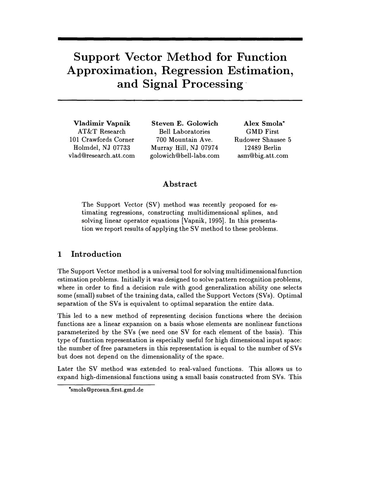
Cover for Support Vector Method for Function Approximation, Regression Estimation and Signal Processing

Abstract

The Support Vector (SV) method was recently proposed for estimating regressions, constructing multidimensional splines, and solving linear operator equations [Vapnik, 1995]. In this presentation we report results of applying the SV method to these problems.

Table of Contents

  • 1 Introduction
  • 2 SV method for estimation of real functions
  • 3 Constructing kernels for inner products
  • 3.1 Kernels generating splines
  • 3.2 Kernels generating Fourier expansions
  • 4 Function estimation and data compression
  • 5 Solution of the linear operator equations
  • 6 Conclusion
  • Acknowledgments
  • References

Knowls

  1. Knowl 1 — Support Vector Regression with ε-Insensitive Loss

    model/method

    The Support Vector (SV) method estimates a real-valued function f(x,w)=i=1wiϕi(x)=(w,Φ(x))+bf(x, w) = \sum_{i=1}^\infty w_i \phi_i(x) = (w, \Phi(x)) + b on training data (x1,y1),,(x,y)(x_1, y_1), \dots, (x_\ell, y_\ell) where xiRnx_i \in \mathbb{R}^n and yiRy_i \in \mathbb{R} by minimizing the regularized risk functional:

    R(w)=1i=1yif(xi,w)ϵ+γ(w,w)R(w) = \frac{1}{\ell} \sum_{i=1}^\ell |y_i - f(x_i, w)|_\epsilon + \gamma (w, w)

    where γ>0\gamma > 0 is a regularization parameter, (w,w)(w, w) denotes the Hilbert space inner product, and ϵ|\cdot|_\epsilon is the ϵ\epsilon-insensitive loss function:

    yf(x,w)ϵ={0if yf(x,w)<ϵyf(x,w)ϵotherwise|y - f(x, w)|_\epsilon = \begin{cases} 0 & \text{if } |y - f(x, w)| < \epsilon \\ |y - f(x, w)| - \epsilon & \text{otherwise} \end{cases}

    The dual quadratic optimization problem maximizes:

    W(α,α)=ϵi=1(αi+αi)+i=1yi(αiαi)12i,j=1(αiαi)(αjαj)K(xi,xj)W(\alpha^*, \alpha) = -\epsilon \sum_{i=1}^\ell (\alpha_i^* + \alpha_i) + \sum_{i=1}^\ell y_i (\alpha_i^* - \alpha_i) - \frac{1}{2} \sum_{i,j=1}^\ell (\alpha_i^* - \alpha_i)(\alpha_j^* - \alpha_j) K(x_i, x_j)

    subject to the linear constraints:

    i=1(αiαi)=0,0αi,αiC(i=1,,)\sum_{i=1}^\ell (\alpha_i^* - \alpha_i) = 0, \quad 0 \le \alpha_i, \alpha_i^* \le C \quad (i = 1, \dots, \ell)

    where CC is a constant determined by γ\gamma, and K(xi,xj)=(Φ(xi),Φ(xj))K(x_i, x_j) = (\Phi(x_i), \Phi(x_j)) is a symmetric positive definite kernel satisfying Mercer's condition K(u,v)g(u)g(v)dudv>0\int K(u, v) g(u) g(v) \, du \, dv > 0 for all non-zero gg. The resulting function depends only on the support vectors where (αiαi)0(\alpha_i^* - \alpha_i) \ne 0:

    f(x,α,α)=i=1(αiαi)K(x,xi)+bf(x, \alpha, \alpha^*) = \sum_{i=1}^\ell (\alpha_i^* - \alpha_i) K(x, x_i) + b

    with αi,αi0\alpha_i^*, \alpha_i \ge 0 and αiαi=0\alpha_i^* \alpha_i = 0.

  2. Knowl 2 — Support Vector Method for Solving Linear Operator Equations

    model/method

    To solve a linear operator equation Af(t)=F(x)A f(t) = F(x), where f(t)Ξf(t) \in \Xi and F(x)ΨF(x) \in \Psi, based on discrete, noisy observations of the right-hand side (x1,F1),,(x,F)(x_1, F_1), \dots, (x_\ell, F_\ell), the unknown function f(t)f(t) is represented in a feature space {ϕr(t)}r=0\{\phi_r(t)\}_{r=0}^\infty as:

    f(t,w)=r=0wrϕr(t)=(w,Φ(t))f(t, w) = \sum_{r=0}^\infty w_r \phi_r(t) = (w, \Phi(t))

    Applying the linear operator AA maps this set into functions:

    F(x,w)=Af(t,w)=r=0wrAϕr(t)=r=0wrψr(x)=(w,Ψ(x))F(x, w) = A f(t, w) = \sum_{r=0}^\infty w_r A \phi_r(t) = \sum_{r=0}^\infty w_r \psi_r(x) = (w, \Psi(x))

    where ψr(x)=Aϕr(t)\psi_r(x) = A \phi_r(t). Solving the inverse problem is equivalent to regression estimation on (xi,Fi)(x_i, F_i) using the image space kernel:

    K(xi,xj)=r=0ψr(xi)ψr(xj)=(Ψ(xi),Ψ(xj))K(x_i, x_j) = \sum_{r=0}^\infty \psi_r(x_i) \psi_r(x_j) = (\Psi(x_i), \Psi(x_j))

    Fitting this SV regression yields coefficients (αiαi)(\alpha_i^* - \alpha_i) for i=1,,i = 1, \dots, \ell. The approximation to the original solution f(t)f(t) is then reconstructed using the cross-kernel function Kc(xi,t)=(Ψ(xi),Φ(t))=r=0ψr(xi)ϕr(t)K_c(x_i, t) = (\Psi(x_i), \Phi(t)) = \sum_{r=0}^\infty \psi_r(x_i) \phi_r(t):

    f(t,α)=i=1(αiαi)Kc(xi,t)f(t, \alpha) = \sum_{i=1}^\ell (\alpha_i^* - \alpha_i) K_c(x_i, t)

  3. Knowl 3 — Reproducing Kernels for Finite-Node and Infinite-Node Polynomial Splines

    equation

    Splines of order nn on [0,1][0, 1] can be represented as linear functions in reproducing kernel Hilbert spaces:

    1. Finite Nodes: For fixed nodes t1,,tN[0,1]t_1, \dots, t_N \in [0, 1] in the basis {1,x,,xn,(xt1)+n,,(xtN)+n}\{1, x, \dots, x^n, (x - t_1)_+^n, \dots, (x - t_N)_+^n\}, where (xt)+=max(xt,0)(x - t)_+ = \max(x - t, 0), the generating kernel is:

    K(xi,xj)=r=0nxirxjr+s=1N(xits)+n(xjts)+nK(x_i, x_j) = \sum_{r=0}^n x_i^r x_j^r + \sum_{s=1}^N (x_i - t_s)_+^n (x_j - t_s)_+^n

    1. Infinite Nodes (Sn()S_n^{(\infty)}): With a continuous distribution of nodes across [0,1][0, 1], the inner product kernel becomes:

    K(xi,xj)=r=0nxirxjr+01(xit)+n(xjt)+ndtK(x_i, x_j) = \sum_{r=0}^n x_i^r x_j^r + \int_0^1 (x_i - t)_+^n (x_j - t)_+^n \, dt

    For one-dimensional linear splines (n=1n = 1), this integrates to:

    K(xi,xj)=1+xixj+xixjmin(xi,xj)xi+xj2(min(xi,xj))2+(min(xi,xj))33K(x_i, x_j) = 1 + x_i x_j + x_i x_j \min(x_i, x_j) - \frac{x_i + x_j}{2} (\min(x_i, x_j))^2 + \frac{(\min(x_i, x_j))^3}{3}

    1. Multidimensional Splines: For mm-dimensional inputs ui=(xi(1),,xi(m))u_i = (x_i^{(1)}, \dots, x_i^{(m)}) and uj=(xj(1),,xj(m))u_j = (x_j^{(1)}, \dots, x_j^{(m)}), the generating kernel is the tensor product of the one-dimensional kernels:

    K(ui,uj)=k=1mK(xi(k),xj(k))K(u_i, u_j) = \prod_{k=1}^m K(x_i^{(k)}, x_j^{(k)})

  4. Knowl 4 — Reproducing Kernels for B_n-Splines and Fourier Expansions

    equation

    Positive definite generating kernels for BnB_n-splines and Fourier series expansions are given as follows:

    1. BnB_n-Spline Kernel: For BnB_n-splines defined by:

    Bn(x)=r=0n+1(1)rn!(n+1r)(x+n+12r)+nB_n(x) = \sum_{r=0}^{n+1} \frac{(-1)^r}{n!} \binom{n+1}{r} \left(x + \frac{n+1}{2} - r\right)_+^n

    the continuous inner product kernel yields the higher-order spline kernel:

    K(xi,xj)=Bn(xit)Bn(xjt)dt=B2n+1(xixj)K(x_i, x_j) = \int_{-\infty}^\infty B_n(x_i - t) B_n(x_j - t) \, dt = B_{2n+1}(x_i - x_j)

    1. Fourier Expansion Kernel: For expansions in the (2N+1)(2N + 1)-dimensional subspace spanned by {12,cosx,sinx,,cosNx,sinNx}\{\frac{1}{\sqrt{2}}, \cos x, \sin x, \dots, \cos Nx, \sin Nx\}, the inner product is given by the Dirichlet kernel:

    K(xi,xj)=12+r=1N(cos(rxi)cos(rxj)+sin(rxi)sin(rxj))=sin((N+1/2)(xixj))2sin(xixj2)K(x_i, x_j) = \frac{1}{2} + \sum_{r=1}^N (\cos(r x_i) \cos(r x_j) + \sin(r x_i) \sin(r x_j)) = \frac{\sin\left((N + 1/2)(x_i - x_j)\right)}{2 \sin\left(\frac{x_i - x_j}{2}\right)}

  5. Knowl 5 — Data Compression in Sinc Function Approximation via ε-Insensitive Splines

    empirical result

    Approximating noiseless samples of the sinc function using infinite-node linear splines S1()S_1^{(\infty)} illustrates how the ϵ\epsilon-insensitive SV method achieves data compression:

    • 1D Sinc Function (f(x)=sinxxf(x) = \frac{\sin|x|}{|x|} sampled on a 100-point uniform lattice):

      • With accuracy ϵ=0.02\epsilon = 0.02, the SV method uses 31 support vectors.
      • With accuracy ϵ=0.1\epsilon = 0.1, the SV method uses 9 support vectors.
    • 2D Sinc Function (f(x,y)=sincx2+y2f(x, y) = \text{sinc}\sqrt{x^2 + y^2} sampled on a 2,500-point uniform lattice):

      • With accuracy ϵ=0.01\epsilon = 0.01, the 2D linear spline requires 157 support vectors, compressing 2,500 data points into 157 parameters.
  6. Knowl 6 — Tomographic Image Reconstruction from Radon Projections Using SV Operator Inversion

    empirical result

    The Support Vector linear operator equation method was applied to image reconstruction from Radon transform projections resembling Positron Emission Tomography (PET):

    a(m)a(m)f(mcosμ+usinμ,msinμucosμ)du=p(m,μ)\int_{-a(m)}^{a(m)} f(m \cos \mu + u \sin \mu, m \sin \mu - u \cos \mu) \, du = p(m, \mu)

    where 1m1-1 \le m \le 1, 0<μ<π0 < \mu < \pi, a(m)=1m2a(m) = \sqrt{1 - m^2}, and observations pi=p(mi,μi)+ξip_i = p(m_i, \mu_i) + \xi_i contain zero-mean noise with E[ξi2]<\mathbb{E}[\xi_i^2] < \infty.

    Using 2D linear splines S1()S_1^{(\infty)}, analytical expressions for the image kernel K(xi,xj)K(x_i, x_j) and cross-kernel Kc(xi,t)K_c(x_i, t) were employed. The continuous target image was reconstructed from 2,048 projection measurements using 172 support vectors (support lines). This continuous kernel representation avoids the standard discrete pixel grid approach, which requires estimating 10,000 to 60,000 parameters.

Coverage note — None was omitted; all key theoretical formulations, kernel derivations, and empirical demonstrations are fully covered.

References

  1. 1.Vladimir Vapnik, "The Nature of Statistical Learning Theory", 1995, Springer Verlag N.Y., 189 p.
  2. 2.Michael Unser and Akram Aldroubi, "Polynomial Splines and Wevelets - A Signal Perspectives", In the book: "Wavelets -A tutorial in Theory and Applications", C.K. Chui (ed) pp. 91 - 122, 1992 Academic Press, Inc.
  3. 3.L. Shepp, Y. Vardi, and L. Kaufman, "A statistical model for Positron Emission Tomography," J. Amer. Stat. Assoc. 80:389 pp. 8-37 1985.

Citation

MLA
Vapnik, V., et al. “Support Vector Method for Function Approximation, Regression Estimation and Signal Processing”. Advances in Neural Information Processing Systems, vol. 9, 1996, pp. 281–87, https://proceedings.neurips.cc/paper_files/paper/1996/file/4f284803bd0966cc24fa8683a34afc6e-Paper.pdf.
APA
Vapnik, V., Golowich, S., & Smola, A. (1996). Support Vector Method for Function Approximation, Regression Estimation and Signal Processing. Advances in Neural Information Processing Systems, 9, 281–287. https://proceedings.neurips.cc/paper_files/paper/1996/file/4f284803bd0966cc24fa8683a34afc6e-Paper.pdf
Chicago
Vapnik, V., S. Golowich, and A. Smola. 1996. “Support Vector Method for Function Approximation, Regression Estimation and Signal Processing”. Advances in Neural Information Processing Systems 9: 281–87. https://proceedings.neurips.cc/paper_files/paper/1996/file/4f284803bd0966cc24fa8683a34afc6e-Paper.pdf.
Harvard
Vapnik, V., Golowich, S. and Smola, A. (1996) “Support Vector Method for Function Approximation, Regression Estimation and Signal Processing”, Advances in Neural Information Processing Systems. Curran Associates, Inc., pp. 281–287. Available at: https://proceedings.neurips.cc/paper_files/paper/1996/file/4f284803bd0966cc24fa8683a34afc6e-Paper.pdf.
Vancouver
1. Vapnik V, Golowich S, Smola A (1996) Support Vector Method for Function Approximation, Regression Estimation and Signal Processing. In: Advances in Neural Information Processing Systems. Curran Associates, Inc., pp 281–287

BibTeX

@inproceedings{NIPS1996_4f284803,
 author = {Vapnik, Vladimir and Golowich, Steven and Smola, Alex},
 booktitle = {Advances in Neural Information Processing Systems},
 editor = {M.C. Mozer and M. Jordan and T. Petsche},
 pages = {},
 publisher = {MIT Press},
 title = {Support Vector Method for Function Approximation, Regression Estimation and Signal Processing},
 url = {https://proceedings.neurips.cc/paper_files/paper/1996/file/4f284803bd0966cc24fa8683a34afc6e-Paper.pdf},
 volume = {9},
 year = {1996}
}
Metadata:DOI registry

Access the Paper

This paper is available from its original source. Click below to access the PDF.

Open PDF

License: Authors