One-Class SVMs for Document Classification

Larry M. Manevitz
[email protected]
Malik Yousef
[email protected]
Department of Computer Science
University of Haifa
Haifa 31905 Israel

Editors: Nello Cristianini, John Shawe-Taylor and Bob Williamson

Abstract

We implemented versions of the SVM appropriate for one-class classification in the context of information retrieval. The experiments were conducted on the standard Reuters data set.

For the SVM implementation we used both a version of Schölkopf et al. and a somewhat different version of one-class SVM based on identifying "outlier" data as representative of the second-class. We report on experiments with different kernels for both of these implementations and with different representations of the data, including binary vectors, tf-idf representation and a modification called "Hadamard" representation. Then we compared it with one-class versions of the algorithms prototype (Rocchio), nearest neighbor, naive Bayes, and finally a natural one-class neural network classification method based on "bottleneck" compression generated filters.

The SVM approach as represented by Schölkopf was superior to all the methods except the neural network one, where it was, although occasionally worse, essentially comparable. However, the SVM methods turned out to be quite sensitive to the choice of representation and kernel in ways which are not well understood; therefore, for the time being leaving the neural network approach as the most robust.

Keywords: Support Vector Machine, SVM, Neural Network, Compression Neural Network, Text Retrieval, Positive Information

Executive Summary: Real-world information retrieval and document filtering systems often encounter situations where only positive training examples are available. For instance, when tracking a user's web browsing history, an automated system can reliably identify topics or sites the user likes, but it is difficult to identify representative negative examples. Traditional machine learning classifiers rely heavily on both positive and negative data to define category boundaries. Adapting algorithms to learn accurately from purely positive information is critical for personalization, recommendation engines, and targeted filtering.

The article evaluates how well one-class support vector machine algorithms perform on document classification when trained exclusively on positive examples. It directly compares these methods against other single-class approaches, including compression neural networks, nearest neighbor, naive Bayes, and prototype methods.

To conduct the evaluation, the authors tested the models across the ten most frequent categories in the standard Reuters news dataset. For each category, the models were trained using 25% of the positive category documents and evaluated on the remaining 75% of the dataset. The study analyzed two single-class support vector machine formulations: the standard one-class formulation (which separates data points from the origin) and an outlier formulation (which treats data points close to the origin as pseudo-negative examples). The experiments systematically varied mathematical transformation functions (kernels), data representation types (such as binary word indicators and frequency-weighted representations), and feature sizes ranging from 10 to 100 terms.

The findings show that the standard one-class support vector machine achieves the highest unweighted overall performance among all tested methods, reaching an average F1 classification score of 0.519 when using a binary representation, 10 features, and a radial basis kernel. This slightly edges out the compression neural network baseline (0.513) and outperforms standard single-class baselines like naive Bayes (0.425), nearest neighbor (0.423), and prototype filtering (0.426) by roughly 20% to 22%. Second, when evaluated using category-weighted macro averaging, the compression neural network achieved the highest score (0.615), followed by the outlier formulation (0.587) and the one-class formulation (0.572), indicating that neural networks perform particularly well on high-volume categories. Third, the one-class support vector machine proved highly sensitive to input choices: performance dropped drastically when moving from a binary format to frequency-weighted representations, or when increasing feature dimensions beyond 10 to 20 terms.

These results demonstrate that single-class support vector machines are computationally faster and simpler to train than neural networks while offering top-tier classification accuracy. However, their extreme sensitivity creates operational risk. Deploying them in automated production environments without extensive tuning could cause significant performance degradation, whereas compression neural networks offer substantially greater out-of-the-box stability across diverse configurations.

For current operational deployments, organizations requiring stable, low-risk single-class filtering should rely on compression neural networks. Teams seeking the lower computational overhead of support vector machines must carefully calibrate their pipelines, strictly utilizing low feature dimensions and binary word representations. Future research must focus on clarifying why these parameter sensitivities occur and developing automated methods to select feature sizes and thresholds when negative training data is entirely absent.

The primary limitation of this study is its reliance on a single benchmark news corpus and preselected keyword representations. While confidence in the comparative performance across these benchmark conditions is high, practitioners should exercise caution and conduct pilot validations before transferring these parameter settings to other text domains.

1. Introduction

Section Summary: Recent work has shown that support vector machines can achieve strong results in tasks like document classification, but standard approaches require both positive and negative training examples. The authors examine methods that use only positive examples, focusing on a one-class SVM technique and comparing it with alternatives such as a neural-network filter. While the one-class SVM performs well, it proves sensitive to choices of data representation and kernel function, leading the authors to favor the neural-network approach for greater robustness.

Recently, mechanisms related to the Support Vector Machine (SVM) paradigm have produced the dramatically best results for information retrieval, e.g. in experiments as measured over the standard Reuters dataset (Dumais et al., 1998).

However, these studies are based on training using both positive and negative examples, as the basic SVM paradigm suggests. We have been interested, however, in information retrieval using only positive examples for training. This is important in many applications (see Manevitz and Yousef, 2001). Consider, for example, trying to classify sites of "interest" to a web surfer where the only information available is the history of the user's activities. One can envisage identifying typical positive examples by such tracking, but it would be hard to identify representative negative examples. Of course, the absence of negative information entails a price, and one should not expect as good results as when they are available (Dumais et al., 1998, Joachims, 1998).

Since Schölkopf et al. (1999) recently extended the SVM methodology to handle training using only positive information (what they call "one-class" classification), we decided to apply their method to documentation classification and compare it with other one-class methods, including a method we recently developed and studied based on a compression neural network as a filter.

There are many parameters in these methods, including the representation of the data, and the decisions involved in modifying basically two-class methods to one class ones. Our studies are fairly broad although not completely comprehensive; below we describe each of the choices we made.

In the end, it turns out that the suggestion of Schölkopf is quite excellent, substantially better than all other methods except the neural network based one with which it is comparable. Moreover, it is somewhat simpler to implement than the neural network method.

However, it turns out to be surprisingly sensitive to specific choices of representation and kernel in ways which are not very transparent. For example, the method works best with binary representation as opposed to tf-idf or "Hadamard" representations which are known to be superior in other methods. In addition, the proper choice of a kernel is dependent on the number of features in the binary vector. Since the difference in performance is very dramatic based on these choices, this means that the method is not robust without a deeper understanding of these representation issues.

This means that, for the moment, we would prefer the neural network method for reasons of robustness.

2. Document Representations, Data Set and Measurements

Section Summary: The section describes four ways to turn documents into numerical vectors based on the most frequent keywords after basic cleaning: a simple binary check for whether each keyword appears, a count of how often it appears, a tf-idf version that down-weights common words across the whole collection, and a Hadamard product that multiplies a word’s local frequency by its global frequency. These representations were evaluated on the standard Reuters news-article collection by training a separate classifier for each of its ten largest categories, using only a quarter of the positive training examples. Results were reported with the usual precision, recall, and balanced F1 scores.

2.1 Document Representations

We used the following different representations in these experiments:

1. binary representation
2. frequency representation
3. tf-idf representation
4. Hadamard representation

These are defined as follows. List all the words (after "stemming"; i.e. removing suffixes and prefixes to avoid duplicate entries and removing basic "stop" words) in all the training documents sorted by the document-frequency (i.e. the number of documents it appears in). Choose the top $m$ such words according to this "dictionary" frequency (called "keywords"). (See in the sequel for experiments with different values of $m$.)

For binary representation of a specific document, choose the $m$ dimensional binary vector where the $i^{th}$ entry is 1 if the $i^{th}$ keyword appears in the document and 0 if it does not.

For the frequency representation, choose the $m$ dimensional real valued vector, where the $i^{th}$ entry is the normalized frequency of appearance of the $i^{th}$ keyword in the specific document.

For the tf-idf representation ("term frequency inverse document frequency"), choose the $m$ dimensional real valued vector, where the $i^{th}$ entry is given by the formula

$ \text{tf}-\text{idf}(\text{keyword}) = \text{frequency}(\text{keyword}) \cdot [\log \frac{n}{N(\text{keyword})} + 1]. $

where $n$ is the total number of words in the dictionary and $N$ is a function giving the total number of documents the keyword appears in.

The Hadamard product representation was discovered experimentally; it consists of the $m$ dimensional vector where the $i^{th}$ entry is the product of the frequency of the $i^{th}$ keyword in the document and its frequency over all documents (in the training set). See Manevitz and Yousef (2001) for further discussion of this representation. In any case, it is clear that this transformation emphasizes differences between large and small feature entries.

2.2 Data Set and Measurements

To test the above ideas, we applied these filters to the standard Reuters dataset (Lewis, 1997), a preclassified collection of short articles. This is one of the standard test-beds used to test information retrieval algorithms (Dumais et al., 1998).

For each choice of category, we used 25% of the positive data from the training set to train; and then tested the filters on the remaining 75% of the data set. Table 1 shows the ten most frequent categories along with the number of training and test examples in each.

: Table 1: Number of Training/Test Items

\begin{tabular}{|l|l|l|}
\hline
Category Name & Num Train & Num Test \\
\hline
Earn & 966 & 2902 \\
Acquisitions & 590 & 1773 \\
Money-fx & 187 & 563 \\
Grain & 151 & 456 \\
Crude & 155 & 465 \\
Trade & 133 & 401 \\
Interest & 123 & 370 \\
Ship & 65 & 195 \\
Wheat & 62 & 186 \\
Corn & 62 & 184 \\
\hline
\end{tabular}

We treated each of the 10 categories as a binary classification task and evaluated the classifiers for each category separately.

For reporting the results, we used the $F_1$ measure, the recall and the precision values. For text categorization, the effectiveness measure of recall and precision are defined as follows:

$ \text{recall} = \frac{\text{Number of items of category identified}}{\text{Number of category members in test set}} $

$ \text{precision} = \frac{\text{Number of items of category identified}}{\text{Total items assigned to category}} $

Van Rijsbergen (1979) defined the $F_1$-measure as a combination of recall (R) and Precision (P) with an equal weight in the following form: $F_1(\text{R,P}) = \frac{2\text{RP}}{\text{R}+\text{P}}$ (This implies that $F_1$, like R and P, is bounded by 1 and the best results under this measure are the higher values.)

3. SVM for One Class Classification: Separating Data from Origin

Section Summary: The section explains how standard SVM techniques, normally requiring both positive and negative examples, can be adapted for one-class classification using only positive data by designating outliers or the origin in feature space as negatives. It details Schölkopf’s approach, which maps inputs via a kernel and separates them from the origin with maximum margin to enclose most points in a simple region, along with a related outlier method that flags sparse vectors near the origin as negatives before applying ordinary two-class SVM. The authors tested both variants extensively with different kernels, feature representations, and thresholds, concluding that the one-class method performed better overall.

The SVM algorithm as it is usually construed is essentially a two-class algorithm (i.e. one needs negative as well as positive examples). Below we present two modifications, one due to Schölkopf and one we proposed, to allow its use for only positive data. Both mechanisms identify "outliers" amongst the positive examples and use them as negative examples. Below we refer to the Schölkopf method as "one-class" and to the other as "outlier".

We investigated both algorithms under a variety of choices of parameters. Our experiments were more extensive for the one-class SVM which seems to be the superior of the two.

3.1 Schölkopf Methodology

Schölkopf et al. (1999) suggested a method of adapting the SVM methodology to the one-class classification problem. Essentially, after transforming the feature via a kernel, they treat the origin as the only member of the second class. Then using "relaxation parameters" they separate the image of the one class from the origin. Then the standard two-class SVM techniques are employed.

They framed the problem in the following way:

Suppose that a dataset has a probability distribution $P$ in the feature space. Find a "simple" subset $S$ of the feature space such that the probability that a test point from $P$ lies outside $S$ is bounded by some a priori specified value.

Supposing that there is a dataset drawn from an underlying probability distribution $P$, one needs to estimate a "simple" subset $S$ of the input space such that the probability that a test point from $P$ lies outside of $S$ is bounded by some a prior specified $\nu \in (0, 1)$ . The solution for this problem is obtained by estimating a function $f$ which is positive on $S$ and negative on the complement $\overline{S}$. In other words, Schölkopf et al., developed an algorithm which returns a function $f$ that takes the value +1 in a "small" region capturing most of the data vectors, and -1 elsewhere.

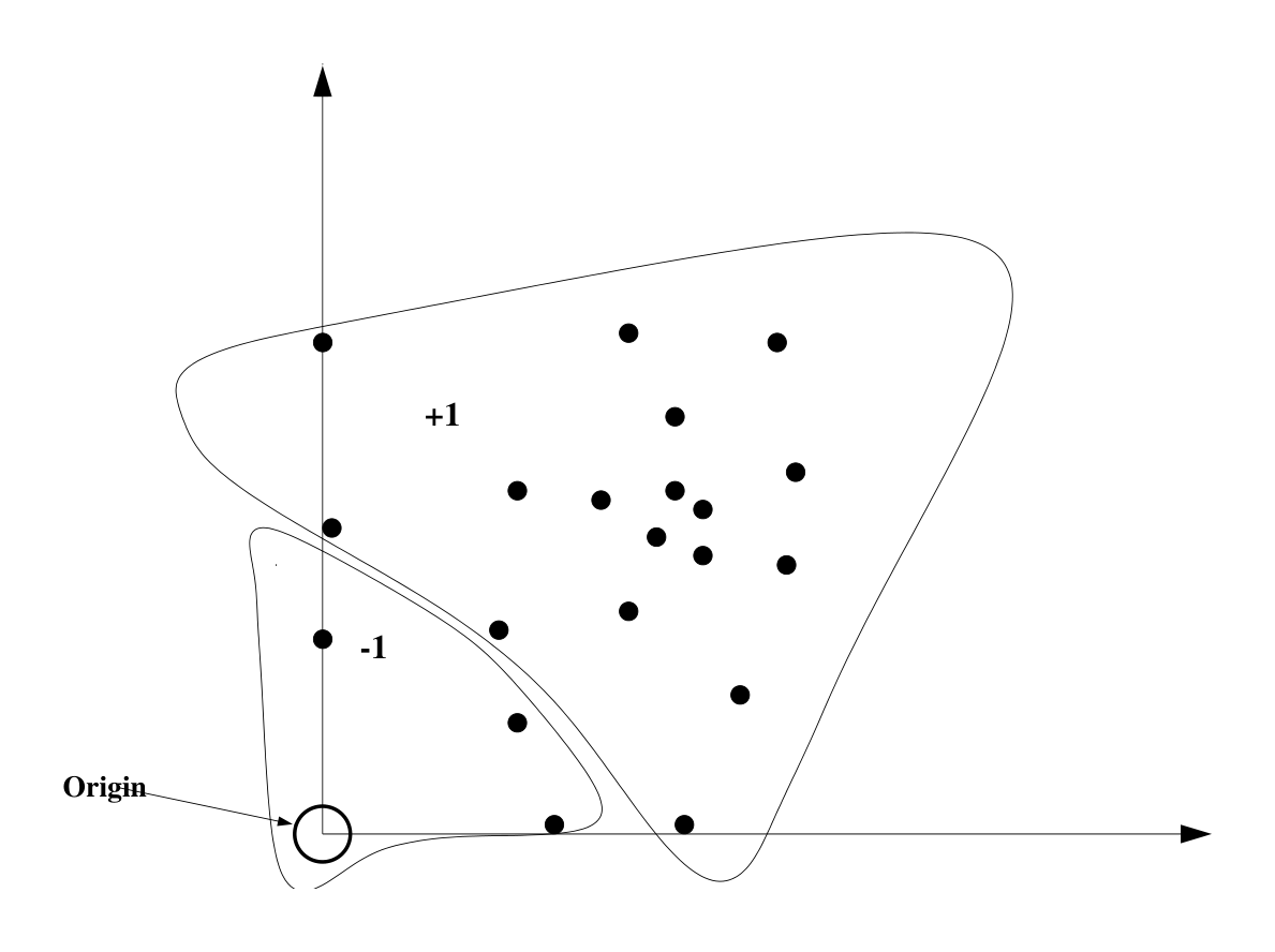
The algorithm can be summarized as mapping the data into a feature space $H$ using an appropriate kernel function, and then trying to separate the mapped vectors from the origin with maximum margin (see Figure 1).

$ f(x) = \begin{cases} +1 & \text{if } x \in S \ -1 & \text{if } x \in \overline{S} \end{cases} $

In our context, let $x_1, x_2, \ldots, x_l$ be training examples belonging to one class $X$, where $X$ is a compact subset of $R^N$. Let $\Phi : X \longrightarrow H$ be a kernel map which transforms the training examples to another space. Then, to separate the data set from the origin, one needs to solve the following quadratic programming problem:

$ \min \frac{1}{2}|w|^2 + \frac{1}{\nu l}\sum_{i=1}^l \xi_i - \rho $

subject to

$ (w \cdot \Phi(x_i)) \geq \rho - \xi_i \quad i = 1, 2, \ldots, l \quad \xi_i \geq 0 $

If $w$ and $\rho$ solve this problem, then the decision function

$ f(x) = \text{sign}((w \cdot \Phi(x)) - \rho) $

will be positive for most examples $x_i$ contained in the training set.

In our research we used the LIBSVM (version 2.0). This is an integrated tool for support vector classification and regression which can handle one-class SVM using the Sholkopf etc algorithms. The LIBSVM 2.0 is available at http://www.csie.ntu.edu.tw/~cjlin/libsvm. We used the standard parameters of the algorithm.

For this "one-class SVM", one has to choose the original frequency representation, (e.g. the number of features), the appropriate kernel, and for each kernel the appropriate parameters. We allowed, linear, sigmoid, polynomial and radial basis kernels; each chosen with the standard parameters. For the original feature representation, we used binary, tf-idf and Hadamard representations. For the number of features we tried 10, 20, 40, 60 and 100 features for the one-class SVM.

3.2 Outlier Methodology

The basic idea is to work first in the feature space, and assume that not only is the origin in the second class (as in the previous section), but also that all data points "close enough" to the origin are to be considered as noise or outliers.

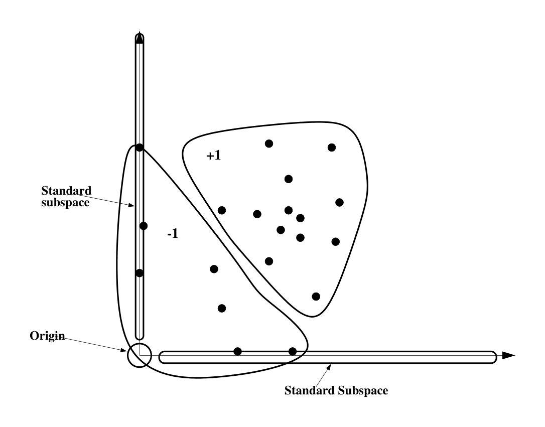
If a vector has few non-zero entries, then this indicates that this document shares very few items with the chosen feature subset of the dictionary. So, intuitively, this item will not serve well as a representative of the class. In this way, it is reasonable to treat such a vector as an outlier. (Note that while the idea of choosing the outliers as data points close to the origin is a general one, the intuitive justification of this procedure is specific to this application.)

Geometrically, using the Hamming distance means that all vectors lying on standard sub-spaces of small dimension (i.e. axes, faces, etc.) are treated as outliers (see Figure 2).

Hence, we decided to identify these outliers by counting the features of an example with non-zero value; and if this is less than a threshold, then the feature is labeled as a negative example.

This raises the problem as to how to choose the appropriate values for the threshold. We investigated this in two ways: (1) by experimentally trying different global values of the threshold and (2) by determining individual thresholds for the different categories. One should note that, in principle, this determination of threshold can be done automatically, e.g. by comparing results on a test set. After having determined the threshold one then continues with the standard two-class SVM.

For this "outlier-SVM", one also has to choose the original frequency representation, and how far from the origin a point can be (in our case, in Hamming distance) before being classified as an outlier.

For the outlier-SVM we tried 10 and 20 features for binary representations. Note that the features are individual category-specific, i.e. different features for each category. (We did sample runs with other representations (e.g. Hadamard, tf-idf) and larger numbers of features, but since the results were clearly poor, we did not complete the experiments.)

In addition, we experimented with varying the Hamming distance in order to define the outlier threshold. Note that this decision can also be chosen automatically (by comparing results on a test set after training) so we also did some statistics over the data set wherein each category had its own such threshold. Table 6 lists the number of documents designated as outliers for each choice of Hamming distance.

We allowed, linear, sigmoid, polynomial and radial basis kernels; each chosen with the "standard" parameters for the two class SVM.

4. Other Methods

Section Summary: In this section the authors outline several established algorithms they will benchmark against their SVM one-class methods, all adapted from an earlier study on the Reuters data set for use with positive examples only. The methods include the simple Prototype (Rocchio) algorithm that averages document vectors, a modified Nearest Neighbor technique, a version of Naive Bayes adjusted to estimate probabilities from positive data alone, and a three-layer neural network with a narrow hidden layer that learns to reconstruct its inputs and thereby identify similar items. These comparisons are presented to allow a consistent evaluation of the SVM approaches.

In recent research (Manevitz and Yousef, 2001) we proposed a one-class neural network classification scheme and compared it over the standard Reuters data set with variants appropriate to the positive example case of several algorithms, using various choices of parameters and various methods of representing the details. For extensive details, see Manevitz and Yousef (2001).

Here we will compare the two SVM one-class algorithms with the following ones from that study:

1. Prototype (Rocchio's) algorithm
   The Prototype algorithm is widely used in information retrieval (Pazzani and Billsus, 1997, Balabanovic and Shoham, 1995, Pazzani et al., 1996, Lang, 1995, and others) . This algorithm is used frequently because it is considered as a baseline algorithm and it is simple to implement. For more details see Joachims (1996).
   The basic idea of the algorithm is to represent each document, e, as a vector in a vector space so that documents with similar content have similar vectors. The value $e_i$ of the $i^{th}$ key-word is represented as the tf-idf weight.
   The Prototype algorithm learns the class model by combining document vectors into a prototype vector . This vector is generated by adding the document vectors of all documents in the class. Classification is done by judging the angular distance from the prototype vector. In our experiments, we used the $F_1$ measure to optimize the threshold.

2. Nearest Neighbor
   This is a modification of the standard Nearest Neighbor algorithm (Yang and Liu, 1999) appropriate for one-class learning. This algorithm was original presented in detail by Datta (1997); and the method of optimizing the parameters is explained by Manevitz and Yousef (2001).

3. Naive Bayes
   Traditional Naive Bayes calculates the probability of being in a class given an example, which has specific values for the different attributes. One calculates this by assuming the different attributes are independent, applying Bayes' theorem and using the a priori probability of the different classes.
   P. Datta (1997) showed how to modify the algorithm for positive data only and we follow his presentation.
   $E$ is the class of training documents in a category. We calculate $p(d|E)$ as the product of $p(w|E)$ for all keywords that appear in the document $d$. Each of the $p(w|E)$ is estimated independently using the formula: $p(w|E) = \frac{n_w+1}{n+m}$ where $n_w$ is the number of times word $w$ occurs in $E$, $n$ is the total number of words in $E$, and $m$ is the number of keywords.
   The threshold is calculated as a fraction (optimized using the $F_1$ measure) of the minimum over all examples in $E$ of the value $p(d|E)$

4. Compression Neural Network
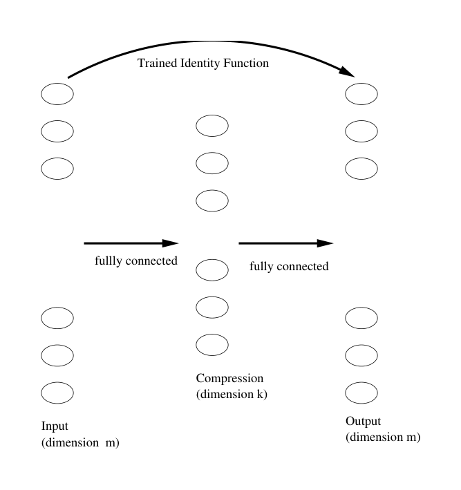
   The algorithm is based on a feed-forward three layer neural network with a "bottleneck". That is, under the assumption that the documents are represented in an $m$-dimensional space; we choose a three level network with $m$ inputs, $m$ outputs and $k$ neurons on the hidden level, where $k < m$. Then the network is trained, under standard back-propagation, to learn the identity function on the sample examples (see Figure 3). This design was first used by G.W. Cottrell and Zipser (1988) to produce a compression algorithm. See also Japkowicz et al. (1995) for another use as a novelty detector.
   The idea is that while the bottleneck prevents learning the full identity function on $m$-space; the identity on the small set of examples is in fact learnable. Then the set of vectors for which the network acts as the identity function is a sort of sub-space which is similar to the trained set. This avoids the "saturation" problem of learning from only positive examples. Thus the filter is defined by applying the network to a given vector; if the result is the identity, then the vector is "interesting".

By running the same experiments using the two SVM-one class algorithms, we are in a position to make a comparative study.

The reader is referred to Manevitz and Yousef (2001) for detailed descriptions of each of the above algorithms and the various choices of parameters investigated.

5. Results

Section Summary: The results section presents performance metrics such as F1 scores, recall, and precision for two SVM-based algorithms across various parameter settings and data representations, with an overall comparison gathered in a summary table. The one-class SVM approach achieved the strongest outcomes under specific conditions, particularly with binary features, a radial basis kernel, and around 10 features per category, although performance proved highly sensitive to changes in these choices. The outlier-SVM variant produced somewhat weaker results in most cases but performed better on larger categories and when averaging across differing category sizes.

We present our results in a series of tables listing the $F_1$, recall and precision values over different parameters. The main summary table is Table 8 where results from all the tables are gathered for comparison.

5.1 One-class SVM (Schölkopf algorithm) Results

The results for this algorithm were very sensitive to the parameters. However, under proper choices it can give the best results.

In particular:

• This algorithm worked much better with the binary representation; in fact the results under all kernels were extremely poor under the other three representations we tested (frequency, tf-idf, and Hadamard). Table 5 presents the Hadamard results with 20 features; results with tf-idf and frequency were equally poor.

• 10 features were best in general, but this depended on the choice of kernel. For polynomial kernel the 20 features were dramatically better. On the other hand, for radial basis kernel 10 features were dramatically better than 20 features (see Table 3).

• Increasing the number of features further caused large decreases in performance (see Table 4).

Aside: Note that the features are category-specific in our approach; unlike other studies such as performed by Joachims (1998), for example. This makes direct dimension comparison difficult. Roughly, the total number of features over all categories in our experiments is about 100 (for twenty features per category).

• We investigated the effect of removing the near-Hamming distance examples from the data set before running this algorithm. We did this for vectors with 10 features. Since the results are worse in all cases in comparison with the original algorithm, we do not reproduce the data tables here.

In summary, the best choice of parameters for this algorithm were 10 features, binary representation with radial basis kernel. However, the sensitivity to changes in any of these parameters makes it difficult to generalize to other applications. The linear kernel, however, while giving somewhat worse results did not seem to be as sensitive.

5.2 Outlier-SVM Results

The results were generally somewhat worse than the one-class SVM results reported above, especially when looked over the array of categories. Occasionally, (e.g. for polynomial kernel with 10 features) this method was superior. Compare Table 3 with Table 2.

For larger categories, outlier-SVM obtained somewhat better results. Using macro averaging (i.e. taking into account the differing number of items in each category), this algorithm reports somewhat better results than the one-class SVM (see Table 8).

• We only tested this algorithm for binary representation.

• 10 features were preferable to 20 features. Compare Table 7 and the subtables in Table 2.

• For 10 features, the best choice of Hamming distance for outlier threshold was 4 or 5. Looking at Table 6 this means that roughly a third of the data were specified as outliers. This indicates that it would be useful to find a better criteria for the original specification of keywords. This is somewhat difficult because in our context only positive information is available.

: Table 2: $F_1$ Values for the Outlier-SVM with different kernels. All with binary representation and vector dimension 10. The number in the first row indicates the number of non-zero feature entries which is required to consider an object an outlier.

\begin{tabular}{|l|l|l|l|l|l|l||l|l|l|l|l|l|l|}
\multicolumn{7}{l}{Linear kernel} & \multicolumn{7}{l}{Polynomial kernel} \\
\hline
 & 3 & 4 & 5 & 6 & 7 & Optimal & & 3 & 4 & 5 & 6 & 7 & Optimal \\
 & $F_1$ & $F_1$ & $F_1$ & $F_1$ & $F_1$ & $F_1$ & & $F_1$ & $F_1$ & $F_1$ & $F_1$ & $F_1$ & $F_1$ \\
\hline
Earn & 0.689 & 0.750 & 0.712 & 0.586 & 0.446 & 0.750 & Earn & 0.718 & 0.784 & 0.705 & 0.584 & 0.445 & 0.784 \\
Acq & 0.488 & 0.504 & 0.450 & 0.323 & 0.195 & 0.504 & Acq & 0.319 & 0.484 & 0.414 & 0.283 & 0.088 & 0.484 \\
Money & 0.492 & 0.563 & 0.508 & 0.425 & 0.292 & 0.563 & Money & 0.111 & 0.522 & 0.448 & 0.397 & 0.221 & 0.522 \\
Grain & 0.444 & 0.523 & 0.481 & 0.283 & 0.133 & 0.523 & Grain & 0.093 & 0.468 & 0.270 & 0.152 & 0.042 & 0.468 \\
Crude & 0.199 & 0.359 & 0.474 & 0.371 & 0.275 & 0.474 & Crude & 0.091 & 0.540 & 0.540 & 0.338 & 0.271 & 0.540 \\
Trade & 0.352 & 0.423 & 0.348 & 0.346 & 0.313 & 0.423 & Trade & 0.078 & 0.078 & 0.451 & 0.327 & 0.273 & 0.451 \\
Int & 0.308 & 0.455 & 0.465 & 0.422 & 0.298 & 0.465 & Int & 0.073 & 0.346 & 0.480 & 0.354 & 0.096 & 0.480 \\
Ship & 0.402 & 0.287 & 0.265 & 0.142 & 0.040 & 0.402 & Ship & 0.115 & 0.078 & 0.020 & 0.000 & 0.000 & 0.115 \\
Wheat & 0.271 & 0.389 & 0.265 & 0.188 & 0.162 & 0.389 & Wheat & 0.036 & 0.036 & 0.192 & 0.168 & 0.125 & 0.192 \\
Corn & 0.228 & 0.332 & 0.306 & 0.356 & 0.185 & 0.356 & Corn & 0.037 & 0.037 & 0.325 & 0.294 & 0.157 & 0.325 \\
\hline
Average & 0.387 & 0.458 & 0.427 & 0.344 & 0.233 & 0.484 & Average & 0.167 & 0.337 & 0.384 & 0.289 & 0.171 & 0.436 \\
\hline
\end{tabular}
\begin{tabular}{|l|l|l|l|l|l|l||l|l|l|l|l|l|l|}
\multicolumn{7}{l}{Radial kernel} & \multicolumn{7}{l}{Sigmoid kernel} \\
\hline
 & 3 & 4 & 5 & 6 & 7 & Optimal & & 3 & 4 & 5 & 6 & 7 & Optimal \\
 & $F_1$ & $F_1$ & $F_1$ & $F_1$ & $F_1$ & $F_1$ & & $F_1$ & $F_1$ & $F_1$ & $F_1$ & $F_1$ & $F_1$ \\
\hline
Earn & 0.688 & 0.751 & 0.712 & 0.586 & 0.440 & 0.751 & Earn & 0.668 & 0.756 & 0.723 & 0.581 & 0.431 & 0.756 \\
Acq & 0.488 & 0.503 & 0.449 & 0.304 & 0.117 & 0.503 & Acq & 0.439 & 0.475 & 0.443 & 0.298 & 0.071 & 0.475 \\
Money & 0.462 & 0.578 & 0.538 & 0.437 & 0.269 & 0.578 & Money & 0.468 & 0.535 & 0.525 & 0.431 & 0.038 & 0.535 \\
Grain & 0.502 & 0.574 & 0.460 & 0.228 & 0.025 & 0.574 & Grain & 0.429 & 0.547 & 0.448 & 0.155 & 0.000 & 0.547 \\
Crude & 0.128 & 0.357 & 0.541 & 0.376 & 0.237 & 0.541 & Crude & 0.124 & 0.382 & 0.494 & 0.372 & 0.257 & 0.494 \\
Trade & 0.352 & 0.429 & 0.380 & 0.275 & 0.278 & 0.429 & Trade & 0.362 & 0.449 & 0.377 & 0.268 & 0.292 & 0.449 \\
Int & 0.253 & 0.441 & 0.457 & 0.365 & 0.092 & 0.457 & Int & 0.190 & 0.397 & 0.472 & 0.291 & 0.000 & 0.472 \\
Ship & 0.327 & 0.333 & 0.142 & 0.040 & 0.000 & 0.333 & Ship & 0.333 & 0.327 & 0.050 & 0.000 & 0.000 & 0.333 \\
Wheat & 0.036 & 0.271 & 0.253 & 0.230 & 0.218 & 0.271 & Wheat & 0.036 & 0.261 & 0.221 & 0.213 & 0.129 & 0.261 \\
Corn & 0.142 & 0.315 & 0.351 & 0.357 & 0.215 & 0.357 & Corn & 0.037 & 0.337 & 0.344 & 0.313 & 0.177 & 0.344 \\
\hline
Average & 0.337 & 0.455 & 0.428 & 0.319 & 0.189 & 0.479 & Average & 0.308 & 0.446 & 0.409 & 0.292 & 0.139 & 0.466 \\
\hline
\end{tabular}

: Table 3: One-class SVM using the binary representation.

\begin{tabular}{|l|l|l|l||l|l|l||l|l|l||l|l|l|}
\multicolumn{13}{l}{Vector Dimension 10} \\
\hline
 & \multicolumn{3}{l||}{Linear} & \multicolumn{3}{l||}{Sigmoid} & \multicolumn{3}{l||}{Polynomial} & \multicolumn{3}{l|}{Radial basis} \\
 & $F_1$ & R & P & $F_1$ & R & P & $F_1$ & R & P & $F_1$ & R & P \\
\hline
Earn & 0.676 & 0.534 & 0.912 & 0.702 & 0.566 & 0.924 & 0.409 & 0.547 & 0.326 & 0.676 & 0.534 & 0.921 \\
Acq & 0.483 & 0.489 & 0.477 & 0.481 & 0.483 & 0.478 & 0.185 & 0.391 & 0.121 & 0.482 & 0.491 & 0.474 \\
Money & 0.541 & 0.504 & 0.585 & 0.516 & 0.451 & 0.604 & 0.074 & 0.481 & 0.040 & 0.514 & 0.481 & 0.552 \\
Grain & 0.585 & 0.447 & 0.846 & 0.533 & 0.388 & 0.850 & 0.084 & 0.491 & 0.046 & 0.585 & 0.447 & 0.846 \\
Crude & 0.545 & 0.490 & 0.614 & 0.532 & 0.470 & 0.611 & 0.441 & 0.462 & 0.423 & 0.544 & 0.490 & 0.613 \\
Trade & 0.445 & 0.376 & 0.545 & 0.476 & 0.396 & 0.597 & 0.363 & 0.463 & 0.299 & 0.597 & 0.492 & 0.433 \\
Int & 0.473 & 0.410 & 0.558 & 0.454 & 0.367 & 0.593 & 0.145 & 0.483 & 0.085 & 0.485 & 0.440 & 0.541 \\
Ship & 0.563 & 0.600 & 0.531 & 0.518 & 0.471 & 0.575 & 0.025 & 0.471 & 0.013 & 0.539 & 0.564 & 0.516 \\
Wheat & 0.474 & 0.376 & 0.642 & 0.450 & 0.365 & 0.586 & 0.619 & 0.516 & 0.774 & 0.474 & 0.376 & 0.642 \\
Corn & 0.293 & 0.380 & 0.238 & 0.339 & 0.380 & 0.307 & 0.036 & 0.440 & 0.019 & 0.298 & 0.391 & 0.240 \\
\hline
Avg & 0.507 & 0.460 & 0.594 & 0.500 & 0.433 & 0.612 & 0.238 & 0.474 & 0.214 & 0.519 & 0.470 & 0.577 \\
\hline
\multicolumn{13}{l}{Vector Dimension 20} \\
\hline
 & \multicolumn{3}{l||}{Linear} & \multicolumn{3}{l||}{Sigmoid} & \multicolumn{3}{l||}{Polynomial} & \multicolumn{3}{l|}{Radial basis} \\
 & $F_1$ & R & P & $F_1$ & R & P & $F_1$ & R & P & $F_1$ & R & P \\
\hline
Earn & 0.652 & 0.521 & 0.873 & 0.686 & 0.562 & 0.880 & 0.678 & 0.555 & 0.871 & 0.321 & 0.479 & 0.241 \\
Acq & 0.488 & 0.495 & 0.481 & 0.489 & 0.497 & 0.482 & 0.491 & 0.482 & 0.501 & 0.194 & 0.465 & 0.122 \\
Money & 0.487 & 0.470 & 0.504 & 0.494 & 0.479 & 0.509 & 0.503 & 0.428 & 0.611 & 0.084 & 0.541 & 0.045 \\
Grain & 0.504 & 0.467 & 0.548 & 0.504 & 0.467 & 0.548 & 0.487 & 0.412 & 0.596 & 0.071 & 0.480 & 0.038 \\
Crude & 0.496 & 0.430 & 0.586 & 0.496 & 0.430 & 0.588 & 0.485 & 0.408 & 0.599 & 0.111 & 0.589 & 0.062 \\
Trade & 0.441 & 0.359 & 0.571 & 0.441 & 0.361 & 0.566 & 0.453 & 0.366 & 0.592 & 0.239 & 0.496 & 0.157 \\
Int & 0.440 & 0.456 & 0.424 & 0.425 & 0.429 & 0.420 & 0.425 & 0.356 & 0.528 & 0.092 & 0.518 & 0.050 \\
Ship & 0.220 & 0.517 & 0.139 & 0.219 & 0.517 & 0.139 & 0.310 & 0.410 & 0.250 & 0.025 & 0.405 & 0.013 \\
Wheat & 0.449 & 0.392 & 0.525 & 0.449 & 0.392 & 0.525 & 0.420 & 0.338 & 0.552 & 0.097 & 0.548 & 0.053 \\
Corn & 0.376 & 0.356 & 0.395 & 0.376 & 0.358 & 0.395 & 0.352 & 0.282 & 0.468 & 0.029 & 0.673 & 0.015 \\
\hline
Avg & 0.455 & 0.446 & 0.504 & 0.458 & 0.449 & 0.505 & 0.460 & 0.403 & 0.557 & 0.126 & 0.519 & 0.079 \\
\hline
\end{tabular}

: Table 4: One-class SVM using the binary representation, with different vector dimensions. Some sample categories.

\begin{tabular}{|l|l|l|l||l|l|l||l|l|l||l|l|l|}
\hline
 & \multicolumn{3}{l||}{Linear} & \multicolumn{3}{l||}{Sigmoid} & \multicolumn{3}{l||}{Polynomial} & \multicolumn{3}{l|}{Radial basis} \\
 & $F_1$ & R & P & $F_1$ & R & P & $F_1$ & R & P & $F_1$ & R & P \\
\hline
\multicolumn{13}{|l|}{dimension 40} \\
\hline
Grain & 0.479 & 0.453 & 0.707 & 0.425 & 0.331 & 0.594 & 0.059 & 0.524 & 0.031 & 0.478 & 0.453 & 0.506 \\
Ship & 0.135 & 0.482 & 0.078 & 0.203 & 0.205 & 0.202 & 0.027 & 0.589 & 0.014 & 0.135 & 0.482 & 0.078 \\
Wheat & 0.416 & 0.392 & 0.442 & 0.307 & 0.226 & 0.482 & 0.030 & 0.548 & 0.015 & 0.414 & 0.392 & 0.439 \\
Corn & 0.340 & 0.380 & 0.308 & 0.325 & 0.250 & 0.464 & 0.029 & 0.625 & 0.015 & 0.339 & 0.380 & 0.307 \\
\hline
\multicolumn{13}{|l|}{dimension 60} \\
\hline
Grain & 0.436 & 0.434 & 0.438 & 0.398 & 0.300 & 0.593 & 0.056 & 0.486 & 0.029 & 0.434 & 0.434 & 0.435 \\
Ship & 0.177 & 0.400 & 0.114 & 0.229 & 0.169 & 0.358 & 0.029 & 0.671 & 0.014 & 0.178 & 0.405 & 0.014 \\
Wheat & 0.383 & 0.381 & 0.385 & 0.254 & 0.182 & 0.419 & 0.028 & 0.591 & 0.014 & 0.388 & 0.387 & 0.389 \\
Corn & 0.326 & 0.347 & 0.307 & 0.272 & 0.195 & 0.450 & 0.027 & 0.592 & 0.013 & 0.324 & 0.347 & 0.303 \\
\hline
\multicolumn{13}{|l|}{dimension 100} \\
\hline
Grain & 0.412 & 0.425 & 0.400 & 0.259 & 0.157 & 0.727 & 0.031 & 0.232 & 0.017 & 0.412 & 0.425 & 0.400 \\
Ship & 0.164 & 0.446 & 0.100 & 0.150 & 0.092 & 0.400 & 0.028 & 0.625 & 0.014 & 0.164 & 0.446 & 0.100 \\
Wheat & 0.530 & 0.376 & 0.897 & 0.258 & 0.150 & 0.903 & 0.039 & 0.634 & 0.020 & 0.530 & 0.376 & 0.897 \\
Corn & 0.273 & 0.320 & 0.237 & 0.186 & 0.125 & 0.370 & 0.028 & 0.619 & 0.014 & 0.272 & 0.320 & 0.236 \\
\hline
\end{tabular}

: Table 5: One-class SVM using the Hadamard representation, with vector dimension 20 ($m=20$).

\begin{tabular}{|l|l|l|l||l|l|l||l|l|l||l|l|l|}
\hline
 & \multicolumn{3}{l||}{Linear} & \multicolumn{3}{l||}{Sigmoid} & \multicolumn{3}{l||}{Polynomial} & \multicolumn{3}{l|}{Radial basis} \\
 & $F_1$ & R & P & $F_1$ & R & P & $F_1$ & R & P & $F_1$ & R & P \\
\hline
Earn & 0.592 & 0.440 & 0.905 & 0.285 & 0.172 & 0.824 & 0.000 & 0.000 & 0.000 & 0.523 & 0.369 & 0.896 \\
Acq & 0.253 & 0.368 & 0.192 & 0.007 & 0.005 & 0.014 & 0.000 & 0.000 & 0.000 & 0.039 & 0.321 & 0.049 \\
Money & 0.266 & 0.278 & 0.255 & 0.168 & 0.312 & 0.114 & 0.000 & 0.000 & 0.000 & 0.266 & 0.278 & 0.255 \\
Grain & 0.067 & 0.035 & 0.888 & 0.066 & 0.035 & 0.615 & 0.098 & 0.910 & 0.051 & 0.067 & 0.035 & 0.888 \\
Crude & 0.139 & 0.101 & 0.227 & 0.068 & 0.116 & 0.048 & 0.000 & 0.000 & 0.000 & 0.139 & 0.101 & 0.227 \\
Trade & 0.523 & 0.755 & 0.400 & 0.273 & 0.795 & 0.165 & 0.000 & 0.000 & 0.000 & 0.523 & 0.755 & 0.400 \\
Int & 0.149 & 0.083 & 0.704 & 0.169 & 0.102 & 0.487 & 0.000 & 0.000 & 0.000 & 0.162 & 0.094 & 0.583 \\
Ship & 0.150 & 0.707 & 0.084 & 0.105 & 0.641 & 0.057 & 0.000 & 0.000 & 0.000 & 0.150 & 0.707 & 0.084 \\
Wheat & 0.054 & 0.225 & 0.031 & 0.014 & 0.059 & 0.008 & 0.051 & 0.962 & 0.026 & 0.057 & 0.236 & 0.032 \\
Corn & 0.079 & 0.304 & 0.046 & 0.019 & 0.043 & 0.012 & 0.040 & 0.989 & 0.020 & 0.079 & 0.304 & 0.046 \\
\hline
Avg & 0.227 & 0.329 & 0.373 & 0.117 & 0.228 & 0.234 & 0.018 & 0.286 & 0.009 & 0.200 & 0.320 & 0.346 \\
\hline
\end{tabular}

In summary, the best parameters for this algorithm were binary representation, feature length 10, and linear kernel function (there was not much difference from the radial basis kernel).

: Table 6: Cumulative number of negative examples (outliers) used from the training set to train the outlier-SVM classifier.

\begin{tabular}{|l|l||l|l|l|l|l|l|l|}
\multicolumn{9}{l}{Vector Dimension 10} \\
\hline
Category Name & Original & 1 & 2 & 3 & 4 & 5 & 6 & 7 \\
\hline
Earn & 966 & 35 & 144 & 231 & 318 & 451 & 630 & 765 \\
Acquisitions & 590 & 33 & 78 & 157 & 254 & 371 & 467 & 532 \\
Money-fx & 187 & 7 & 26 & 43 & 67 & 101 & 123 & 157 \\
Grain & 151 & 2 & 21 & 37 & 61 & 100 & 122 & 139 \\
Crude & 155 & 1 & 16 & 30 & 55 & 72 & 92 & 110 \\
Trade & 133 & 2 & 9 & 17 & 27 & 50 & 73 & 91 \\
Interest & 123 & 3 & 8 & 19 & 38 & 51 & 84 & 107 \\
Ship & 65 & 8 & 20 & 33 & 46 & 53 & 58 & 63 \\
Wheat & 62 & 1 & 5 & 8 & 23 & 39 & 46 & 49 \\
Corn & 62 & 2 & 7 & 8 & 20 & 30 & 35 & 44 \\
\hline
\multicolumn{9}{l}{Vector Dimension 20} \\
\hline
Category Name & Original & 3 & 4 & 5 & 6 & 7 & 8 & \multicolumn{1}{|l}{} \\
\cline{1-8}
Earn & 966 & 41 & 120 & 235 & 410 & 538 & 650 & \multicolumn{1}{|l}{} \\
Acquisitions & 590 & 98 & 148 & 235 & 311 & 368 & 422 & \multicolumn{1}{|l}{} \\
Money-fx & 187 & 18 & 30 & 48 & 74 & 97 & 118 & \multicolumn{1}{|l}{} \\
Grain & 151 & 13 & 29 & 45 & 68 & 96 & 110 & \multicolumn{1}{|l}{} \\
Crude & 155 & 14 & 23 & 37 & 49 & 65 & 82 & \multicolumn{1}{|l}{} \\
Trade & 133 & 8 & 14 & 18 & 27 & 39 & 51 & \multicolumn{1}{|l}{} \\
Interest & 123 & 11 & 14 & 35 & 45 & 62 & 78 & \multicolumn{1}{|l}{} \\
Ship & 65 & 20 & 31 & 35 & 40 & 47 & 52 & \multicolumn{1}{|l}{} \\
Wheat & 62 & 1 & 7 & 15 & 23 & 32 & 45 & \multicolumn{1}{|l}{} \\
Corn & 62 & 2 & 7 & 9 & 11 & 26 & 32 & \multicolumn{1}{|l}{} \\
\cline{1-8}
\end{tabular}

: Table 7: Outlier-SVM using binary representation with different kernel functions, outliers with Hamming distance 7, vector dimension 20.

\begin{tabular}{|l|l|l|l||l|l|l||l|l|l||l|l|l|}
\hline
 & \multicolumn{3}{l||}{Linear} & \multicolumn{3}{l||}{Sigmoid} & \multicolumn{3}{l||}{Polynomial} & \multicolumn{3}{l|}{Radial basis} \\
 & $F_1$ & R & P & $F_1$ & R & P & $F_1$ & R & P & $F_1$ & R & P \\
\hline
Earn & 0.605 & 0.490 & 0.791 & 0.593 & 0.451 & 0.864 & 0.391 & 0.249 & 0.909 & 0.592 & 0.477 & 0.779 \\
Acq & 0.449 & 0.376 & 0.556 & 0.452 & 0.366 & 0.591 & 0.329 & 0.214 & 0.706 & 0.449 & 0.371 & 0.567 \\
Money & 0.480 & 0.463 & 0.498 & 0.474 & 0.415 & 0.551 & 0.315 & 0.202 & 0.716 & 0.484 & 0.431 & 0.551 \\
Grain & 0.350 & 0.364 & 0.337 & 0.369 & 0.271 & 0.574 & 0.091 & 0.048 & 0.849 & 0.384 & 0.289 & 0.573 \\
Crude & 0.455 & 0.501 & 0.416 & 0.522 & 0.541 & 0.504 & 0.458 & 0.354 & 0.647 & 0.493 & 0.511 & 0.476 \\
Trade & 0.419 & 0.618 & 0.317 & 0.432 & 0.735 & 0.306 & 0.078 & 1.000 & 0.041 & 0.441 & 0.685 & 0.325 \\
Int & 0.390 & 0.391 & 0.388 & 0.378 & 0.321 & 0.461 & 0.137 & 0.075 & 0.736 & 0.379 & 0.332 & 0.440 \\
Ship & 0.280 & 0.189 & 0.536 & 0.221 & 0.128 & 0.806 & 0.000 & 0.000 & 0.000 & 0.236 & 0.143 & 0.666 \\
Wheat & 0.225 & 0.413 & 0.154 & 0.197 & 0.268 & 0.155 & 0.031 & 0.016 & 0.428 & 0.183 & 0.376 & 0.121 \\
Corn & 0.217 & 0.391 & 0.150 & 0.352 & 0.467 & 0.282 & 0.037 & 1.000 & 0.019 & 0.353 & 0.472 & 0.282 \\
\hline
Avg & 0.378 & 0.419 & 0.414 & 0.399 & 0.396 & 0.509 & 0.186 & 0.315 & 0.505 & 0.399 & 0.408 & 0.478 \\
\hline
\end{tabular}

: Table 8: Comparison of One-class SVM (binary representation), Outlier-SVM (binary representation), Neural Networks (Hadamard representation), Naive Bayes, Nearest Neighbor (Hadamard representation), and Prototype Algorithms (tf-idf representation). (Each method with the best representation tested.)

\begin{tabular}{|l|l|l|l|l|l|l|}
\hline
 & One-class & Outlier- & Neural & Naive & Nearest & Prototype \\
 & SVM Radial & SVM & Networks & Bayes & Neighbor & \\
 & Basis & Linear & & & & \\
 & $F_1$ & $F_1$ & $F_1$ & $F_1$ & $F_1$ & $F_1$ \\
\hline
Earn & 0.676 & 0.750 & 0.714 & 0.708 & 0.703 & 0.637 \\
Acq & 0.482 & 0.504 & 0.621 & 0.503 & 0.476 & 0.468 \\
Money & 0.514 & 0.563 & 0.642 & 0.493 & 0.468 & 0.484 \\
Grain & 0.585 & 0.523 & 0.473 & 0.382 & 0.333 & 0.402 \\
Crude & 0.544 & 0.474 & 0.534 & 0.457 & 0.392 & 0.398 \\
Trade & 0.597 & 0.423 & 0.569 & 0.483 & 0.441 & 0.557 \\
Int & 0.485 & 0.465 & 0.487 & 0.394 & 0.295 & 0.454 \\
Ship & 0.539 & 0.402 & 0.361 & 0.288 & 0.389 & 0.370 \\
Wheat & 0.474 & 0.389 & 0.404 & 0.288 & 0.566 & 0.262 \\
Corn & 0.298 & 0.356 & 0.324 & 0.254 & 0.168 & 0.230 \\
\hline
Avg & 0.519 & 0.484 & 0.513 & 0.425 & 0.423 & 0.426 \\
\hline
Macro & 0.572 & 0.587 & 0.615 & 0.547 & 0.530 & 0.516 \\
\hline
\end{tabular}

6. Comparisons and Conclusions

Section Summary: In comparisons across ten Reuters categories, the one-class SVM achieved the strongest overall results on unweighted averages, performing comparably to a neural network method while offering computational advantages over it. Macro averages that account for category size showed stronger results from the neural network and outlier-SVM approaches, which excelled on larger categories, whereas the one-class SVM proved more robust on smaller ones. However, because the one-class SVM proved highly sensitive to parameter and kernel choices while the neural network remained more stable, the authors conclude that the neural network method is currently preferable.

In Table 8, we list the best $F_1$ results from one-class SVM, outlier-SVM and the four other algorithms from the work by Manevitz and Yousef (2001). The results from ten Reuters categories are presented. We also list, in this table, the "macro" averages which take into account the different number of items in each category.

Looking over this table, and focusing on the unweighted average, we see that the one-class SVM as proposed by Schölkopf et al., gives the best overall performance. This is quite clear with respect to all the other algorithms except the compression NN algorithm which is comparable. Schölkopf's proposal has the usual advantages of SVM; in particular it is less computationally intensive than neural networks.

Under the "macro" averaging, the NN and outlier-SVM were somewhat superior. This means that while the one-class SVM was more robust with regards to smaller categories, the NN and outlier-SVM showed good results by emphasizing success in the larger categories.

On the other hand, the one-class SVM was very sensitive to the parameters and choice of kernel. The neural network method, in comparison, seemed relatively stable over these parameters. (In our experiments, the linear kernel was, however, fairly stable although its results were slightly worse than the neural network algorithm.) Thus, under current knowledge, i.e. until understanding of the parameter choice is clearer, it would seem that the neural network method is the preferred one.

Acknowledgments

This work was partially supported by HIACS, the Haifa Interdisciplinary Center for Advanced Computer Science.

References

Section Summary: This section compiles a list of academic papers, technical reports, and theses primarily from the 1980s through early 2000s, centered on machine learning methods for handling text and web information. The works explore techniques such as neural networks, support vector machines, and algorithms for categorizing documents, detecting novelty, or filtering content like news articles. Many cite conferences in artificial intelligence and information retrieval, along with foundational texts on the subject.

M. Balabanovic and Y. Shoham. Learning information retrieval agents: Experiments with automated web browsing. In Working Notes of AAAI Spring Symposium Series on Information Gathering from Distributed, Heterogeneous Environments. AAAI-Press, 1995.

P. Datta. Characteristic Concept Representations. PhD thesis, University of California, Irvine, 1997.

S.T. Dumais, J. Platt, D. Heckerman, and M. Sahami. Inductive learning algorithms and representation for text categorization. In Proceedings of the seventh International Conference on Information and Knowledge Management (CIKM'98), pages 148–155, 1998.

P. Munro G.W. Cottrell and D. Zipser. Image compression by back propagation: an example of extensional programming. In N.E. Sharkey, editor, Advances in Cognitive Science, volume 3. Ablex, 1988.

N. Japkowicz, C. Myers, and M. Gluck. A novelty detection approach to classification. In Proceeding of the Fourteenth International Conference On Artificial Intelligence, pages 518–523. Montreal, Canada, 1995.

T. Joachims. A probabilistic analysis of the Rocchio algorithm with TF-IDF for text categorization. Technical Report CMU-CS-96-118, School of Computer Science, Carnegie Mellon University, Pittsburgh, 1996.

T. Joachims. Text categorization with support vector machines: Learning with many relevant features. In Proceeding 10 European Conference on Machine Learning (ECML), pages 137–142. Springer Verlag, 1998. URL http://www-ai.cs.uni-dortmund.de/DOKIMENTE/Joachims_97a.sp.gz.

K. Lang. NewsWeeder:Learning to filter news. In Twelfth International Conference on Machine Learning, pages 331–339. Lake Tahoe, CA, 1995.

D. Lewis. Reuters-21578 text categorization test collection. http://www.research.att.com/~lewis, 1997.

L. Manevitz and M. Yousef. Document classification via neural networks trained exclusively with positive examples. Technical report, Department of Computer Science, University of Haifa, Haifa, 2001.

M. Pazzani and D. Billsus. Learning and revising user profiles: The identification of interesting web sites. Machine Learning, 27:313–331, 1997.

M. Pazzani, J. Muramatsu, and D. Billsus. Syskill & Webert:Identifying interesting web sites. In AAAI Conference 1996, pages 54–61, 1996.

B. Schölkopf, J.C. Platt, J.Shawe-Taylor, A.J. Smola, and R.C. Williamson. Estimating the support of a high-dimensional distribution. Technical report, Microsoft Research, MSR-TR-99-87, 1999.

C.J. van Rijsbergen. Information Retrieval. Butterworths, London, second edition, 1979.

Yiming Yang and Xin Liu. A re-examination of text categorization methods. In Marti A. Hearst, Fredric Gey, and Richard Tong, editors, Proceedings of SIGIR-99, 22nd ACM International Conference on Research and Development in Information Retrieval, pages 42–49, Berkeley, US, 1999. ACM Press, New York, US. URL http://www.cs.cmu.edu/~yiming/papers.yy/sigir99.ps.