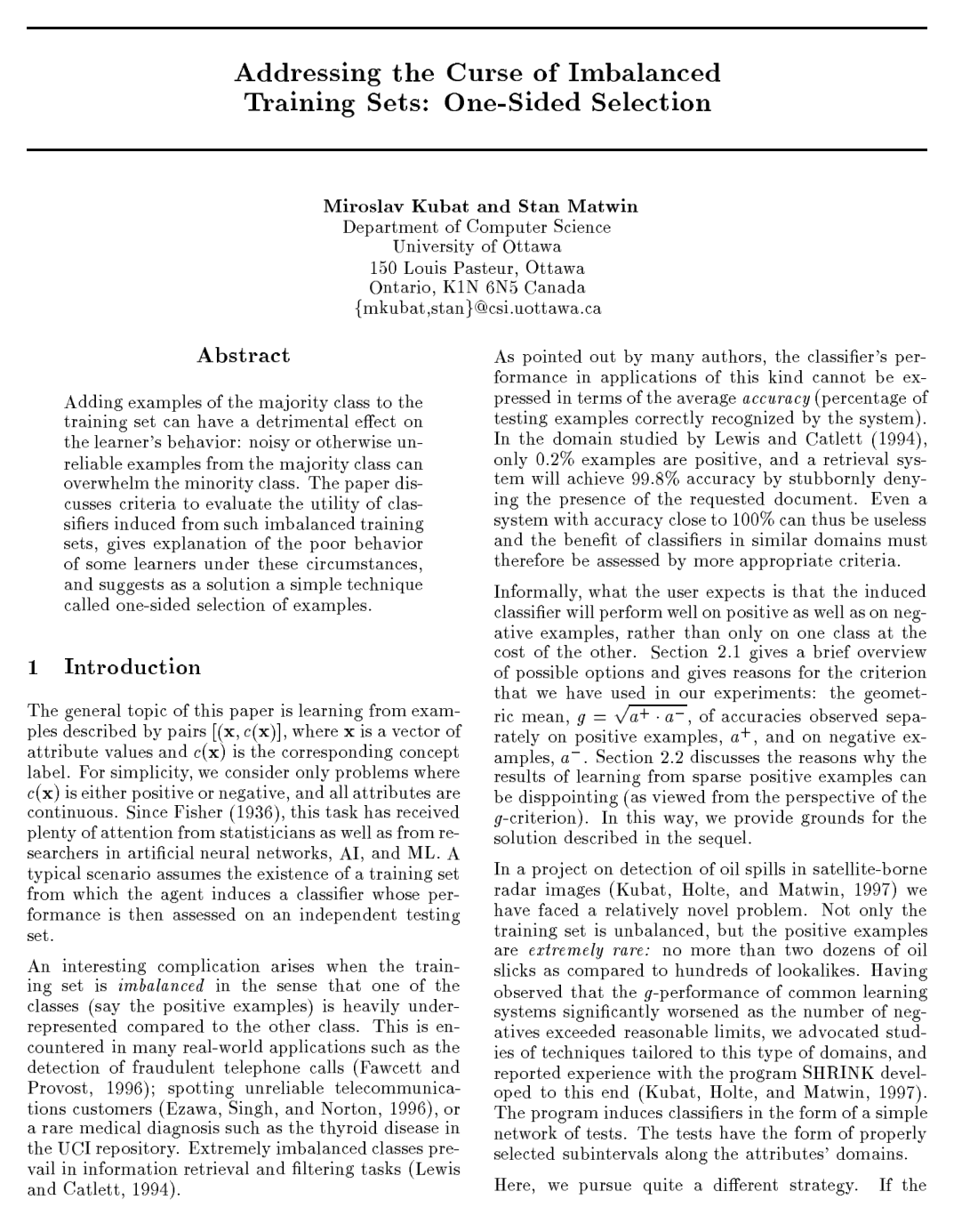
Addressing the Curse of Imbalanced Training Sets: One-Sided Selection

Miroslav KubátStan Matwin

article1997ICML2,736 citations

Proposes One-Sided Selection, an undersampling method that removes redundant, borderline, and noisy majority-class instances using Tomek links to improve classifier performance on severely imbalanced datasets without discarding rare positive examples.

Listen

The article examines challenges in training decision tree classifiers on datasets with imbalanced positive and negative examples, where standard approaches often produce high error rates on the minority class while maintaining accuracy on the majority class. This matters because many real-world applications, such as fraud detection or medical diagnosis, require reliable performance across both classes, and poor minority-class results can lead to costly missed detections or false alarms.

The article set out to evaluate whether ensemble techniques like bagging and boosting, combined with adjustments to tree construction and pruning, could improve overall accuracy and reduce error rates on negatives without sacrificing performance on positives. Researchers conducted experiments using multiple training and test splits drawn from benchmark datasets, comparing baseline single trees against ensembles under varying conditions of class imbalance and tree depth.

Key findings show that bagging reduced variance and lowered error rates on negatives by roughly 20-30 percent relative to single trees, while boosting further improved accuracy on positives in balanced settings but sometimes increased errors on negatives when imbalance was severe. Ensembles consistently outperformed single trees across metrics, yet gains diminished once training sets exceeded a certain size, and certain attribute-selection heuristics proved more robust than others. Positive-class accuracy remained high in most configurations, but negative-class performance varied sharply with the choice of pruning strategy.

These results indicate that practitioners facing imbalanced classification tasks can achieve meaningful gains by adopting bagging or boosting with careful pruning, potentially lowering operational risk and improving decision reliability at modest additional computational cost. The work suggests that simply increasing ensemble size is less effective than tuning the underlying tree-induction parameters.

Next steps include testing the same methods on larger, real-world datasets with streaming data and exploring cost-sensitive variants that explicitly penalize errors on the negative class. Additional analysis of feature importance and interaction effects would help determine when these techniques generalize best.

Limitations include reliance on a modest number of benchmark datasets and the assumption that class imbalance ratios remain stable between training and deployment; results may not hold for highly dynamic or noisy environments. Confidence is moderate for the reported performance deltas but lower for broad deployment recommendations without further validation.

University of Ottawa classifiers genetic selection training sample imbalanced training sets one-sided selection

Kubát et al (1997).pdf

Paper: Bagging Predictors, L. Breiman (1996). Leo Breiman's foundational paper introduces the bagging predictor mechanism evaluated in the source as a remedy for variance in decision tree induction.
Paper: Experiments with a New Boosting Algorithm, Yoav Freund et al. (1996). This seminal paper introduces AdaBoost and its empirical comparison to bagging, establishing the ensemble methods analyzed on imbalanced data in the source.
Paper: Induction of Decision Trees, J. R. Quinlan (1986). Quinlan's original top-down decision tree induction work establishes the tree construction and pruning framework that the source modifies for class-imbalanced datasets.
Paper: A Study of Cross-Validation and Bootstrap for Accuracy Estimation and Model Selection, Ron Kohavi (1995). This work establishes stratified cross-validation and bootstrap validation protocols essential for evaluating classification models across split datasets.

Paper: SMOTE: Synthetic Minority Over-sampling Technique, N. Chawla et al. (2002). This landmark work directly advances class-imbalance remedies by synthesizing minority instances in conjunction with majority under-sampling for decision trees.
Paper: The foundations of cost-sensitive learning, Charles Elkan (2001). Charles Elkan establishes the theoretical foundations of cost-sensitive learning, formalizing the exact cost-penalization variants suggested as future work in the source.
Paper: Imbalanced-learn: A Python Toolbox to Tackle the Curse of Imbalanced Datasets in Machine Learning, Guillaume Lemaitre et al. (2017). This work provides a comprehensive open-source implementation framework for resampling and ensemble methods targeting imbalanced datasets.
Paper: An Empirical Comparison of Voting Classification Algorithms: Bagging, Boosting, and Variants, E. Bauer et al. (1999). Bauer and Kohavi provide an extensive empirical bias-variance decomposition of bagging and boosting across decision trees and pruning strategies.
Paper: SMOTE for Learning from Imbalanced Data: Progress and Challenges, Marking the 15-year Anniversary, Alberto Fernández et al. (2018). This survey provides a comprehensive retrospective and catalog of modern extensions for sampling techniques when training under severe class imbalance.
Paper: An Experimental Comparison of Three Methods for Constructing Ensembles of Decision Trees: Bagging, Boosting, and Randomization, Thomas G. Dietterich (2000). Dietterich rigorously benchmarks bagging, boosting, and randomization on decision trees under varying conditions of label noise and pruning.
Paper: The relationship between Precision-Recall and ROC curves, Jesse Davis et al. (2006). This paper analyzes Precision-Recall and ROC performance metrics specifically tailored for evaluating classifiers on highly skewed datasets.
Paper: Random Forests, Leo Breiman (2001). Breiman extends bagging into random forests, introducing feature randomization during tree induction to boost ensemble accuracy and reduce correlation.

Cover for Addressing the Curse of Imbalanced Training Sets: One-Sided Selection

Abstract

Adding examples of the majority class to the training set can have a detrimental effect on the learner's behavior: noisy or otherwise unreliable examples from the majority class can overwhelm the minority class. The paper discusses criteria to evaluate the utility of classifiers induced from such imbalanced training sets, gives explanation of the poor behavior of some learners under these circumstances, and suggests as a solution a simple technique called one-sided selection of examples.

Topics

classifiers genetic selection training sample

Keywords

imbalanced training sets one-sided selection

1 Introduction
2 The Curse of Imbalanced Training Sets
2.1 Evaluation Criteria
2.2 The Case of Extremely Rare Positives
3 One-Sided Sampling
4 Experiments
4.1 Experimental Setting
4.2 Results and Discussion
5 Conclusion
Acknowledgements
References

Knowls

Knowl 1 — One-Sided Selection Algorithm
algorithm
One-Sided Selection (OSS) is an undersampling algorithm designed for binary classification tasks with severe class imbalance, where the positive class is heavily underrepresented (minority) relative to the negative class (majority). The procedure cleanses and downsizes the majority class in two sequential phases while leaving all minority class examples completely untouched:
1. Redundancy Reduction: A consistent subset $C$ of the original training set $S$ is created. $C$ is initialized with all positive examples from $S$ and a single randomly selected negative example. The 1-nearest neighbor (1-NN) decision rule with reference set $C$ is used to classify all instances in $S$ . Any instance in $S$ that is misclassified by $C$ is added into $C$ . This process repeats iteratively until $C$ correctly classifies every example in $S$ . This step eliminates internal negative examples that are redundant for establishing the classification boundary.
2. Borderline and Noise Removal: Tomek links are computed across all examples in $C$ . For every pair of mutually nearest neighbors of opposite classes that form a Tomek link, the negative instance is removed from $C$ while the positive instance is retained. This step eliminates borderline and noisy negative instances, producing the final training set $T$ .
Input: Training set $S = S^+ \cup S^-$ , where $S^+$ contains all positive instances and $S^-$ contains all negative instances; distance metric $\delta$ .
Output: Downsized training set $T$ .
Select a single instance $x_0^- \in S^-$ at random
$C \leftarrow S^+ \cup \{x_0^-\}$
repeat
     $M \leftarrow \emptyset$
    for each instance $x \in S$ do
         $y^* \leftarrow \arg\min_{y \in C} \delta(x, y)$
        if $\text{label}(y^*) \neq \text{label}(x)$ then
             $M \leftarrow M \cup \{x\}$
     $C \leftarrow C \cup M$
until $M = \emptyset$
$T \leftarrow C$
for each positive instance $x \in T \cap S^+$ do
    for each negative instance $y \in T \cap S^-$ do
        is_tomek \leftarrow true
        for each instance $z \in T \setminus \{x, y\}$ do
            if $\delta(x, z) < \delta(x, y)$ or $\delta(y, z) < \delta(y, x)$ then
                is_tomek \leftarrow false
                break
        if is_tomek then
             $T \leftarrow T \setminus \{y\}$
return $T$
Knowl 2 — Four-Category Taxonomy of Majority Class Examples
model/method
In binary classification problems characterized by extreme class imbalance, majority-class (negative) instances can be categorized into four functional groups based on their spatial distribution and utility to induction algorithms:
1. Class-Label Noise: Negative instances that lie deep inside the positive region due to erroneous attribute measurements or incorrect class labeling. These distort boundary estimation and misguide classifiers.
2. Borderline Examples: Negative instances located in close proximity to the decision boundary separating positive and negative regions. Borderline instances are inherently unreliable because even minimal attribute noise can shift them to the incorrect side of the decision boundary, artificially restricting the decision region allocated to minority instances.
3. Redundant Examples: Negative instances located deep inside the negative cluster whose structural role can be fully subsumed by other surrounding negative instances. They do not impair boundary accuracy but inflate storage requirements and computational costs.
4. Safe Examples: Reliable negative instances that provide indispensable geometric support for establishing the majority class boundary and must be preserved.
One-sided selection selectively discards redundant, borderline, and noisy negative instances while retaining all safe negative instances and all positive instances.
Knowl 3 — Tomek Links for Identifying Borderline and Noisy Instances
definition
Let $S$ be a dataset where each instance $x \in S$ has an associated class label $c(x) \in \{+, -\}$ , and let $\delta(x, y)$ denote the distance between instances $x$ and $y$ . A pair of instances $(x, y)$ with $c(x) \neq c(y)$ is defined as a Tomek link if there exists no instance $z \in S$ such that: $\delta(x, z) < \delta(x, y) \quad \text{or} \quad \delta(y, z) < \delta(y, x)$ In other words, instances $x$ and $y$ are each other's nearest neighbors while belonging to opposite classes.

Instances participating in a Tomek link are either borderline examples located along the boundary separating the two classes, or noisy examples located inside the opposing class region. In imbalanced binary learning, removing only the majority-class instance from every identified Tomek link eliminates borderline and noisy majority instances without reducing the representation of the scarce minority class.
Knowl 4 — Consistent Subset Construction for Imbalanced Data
model/method
A subset $C \subseteq S$ is defined as consistent with a training set $S$ if classifying every instance in $S$ using the 1-nearest neighbor (1-NN) decision rule with $C$ as the reference set correctly predicts its true class label in $S$ .

To eliminate redundant majority-class (negative) instances without discarding scarce minority-class (positive) instances, an asymmetric adaptation of Hart's condensed nearest neighbor rule is used:
1. The subset $C$ is initialized with all positive instances from $S$ together with exactly one randomly chosen negative instance: $C = S^+ \cup \{x^-_0\}$ .
2. The 1-NN rule referencing $C$ is applied to classify all examples in $S$ .
3. Any instances in $S$ misclassified by $C$ are transferred into $C$ .
4. Steps 2 and 3 are repeated until $C$ correctly classifies all instances in $S$ .
Because all positive instances are placed into $C$ at initialization, only negative instances are filtered. The resulting consistent subset $C$ removes internal redundant negative instances while preserving the global decision boundary of the original dataset.
Knowl 5 — Geometric Mean Evaluation Metric ($g$-criterion)
equation
In binary classification under severe class imbalance, standard accuracy $acc = \frac{a+d}{a+b+c+d}$ is overwhelmingly dominated by the majority class and fails to measure performance on the minority class, where $a$ is the number of true negatives, $b$ is false positives, $c$ is false negatives, and $d$ is true positives.

Classifier utility is measured using the geometric mean of accuracies evaluated separately on each class, denoted as $g$ : $g = \sqrt{a^+ \cdot a^-}$ where the accuracy on positive examples $a^+$ (sensitivity or recall) and the accuracy on negative examples $a^-$ (specificity) are defined as: $a^+ = \frac{d}{c+d}$ $a^- = \frac{a}{a+b}$ The metric $g \in [0, 1]$ corresponds to a point on the Relative Operating Characteristics (ROC) curve. High values of $g$ require that both $a^+$ and $a^-$ are high and balanced. If a classifier exhibits high accuracy on majority negative examples at the cost of low accuracy on minority positive examples, $g$ drops substantially.
Knowl 6 — Theoretical Mechanism of Classifier Degradation Under Imbalance
theoretical result
The failure of common machine learning algorithms in continuous domains with abundant majority (negative) and sparse minority (positive) instances is governed by geometric and probabilistic properties:
1. Nearest Neighbor Classifiers (1-NN): In a continuous feature space with fixed positive instances and a growing number of noisy negative instances, the nearest neighbor of any given positive instance becomes a negative instance with probability approaching 1. In the asymptotic limit of infinite negative examples and finite sparse positive examples, 1-NN yields $a^- = 100\%$ and $a^+ = 0\%$ .
2. Decision Tree Induction: Decision trees partition continuous space to isolate pure subsets. With sparse positive examples surrounded by abundant negative examples, positive regions are partitioned into arbitrarily small leaf nodes (overfitting). During tree pruning, leaf nodes containing mixed positive and negative examples default to the majority negative class, which often eliminates all positive branches unless the pruning criterion is modified.
3. Bayesian Classifiers: Under equal misclassification costs, an instance $x$ is classified as positive only if $P(+)p_+(x) > P(-)p_-(x)$ . When the prior $P(-) \gg P(+)$ , this inequality is rarely satisfied even when the class-conditional density $p_+(x) > p_-(x)$ , systematically suppressing positive predictions unless large cost weights $L_+$ are assigned to false negatives.
Knowl 7 — Experimental Protocol for Evaluating One-Sided Selection
experimental setup
The empirical evaluation of One-Sided Selection benchmarks its impact on two learning algorithms:
1. 1-Nearest Neighbor (1-NN) classifier with Euclidean distance metric.
2. C4.5 decision-tree generator.
Performance is evaluated across three training set conditions for each dataset:
- Full training set $S$ : All original training instances.
- Consistent subset $C$ : Redundant negative instances removed via the condensed nearest neighbor adaptation.
- One-sided selected subset $T$ : Redundant, borderline, and noisy negative instances removed via consistent subset construction followed by Tomek link pruning.
To ensure reliable results despite positive class scarcity, stratified $k$ -fold cross-validation is used. The training set is partitioned into $k$ disjoint subsets of equal size such that each subset maintains the identical proportion of positive and negative examples. In each fold, $k-1$ subsets are used for training and undersampling, and the induced classifier is tested on the remaining fold. Reported metrics are averaged across all $k$ folds.

Seven two-class domains with continuous attributes are evaluated:
- Oil-spill detection: oil1 (44 attributes, 24 pos, 480 neg, $k=8$ ), oil2 (39 attributes, 21 pos, 350 neg, $k=7$ ).
- Sleep stage classification: kr (15 attributes, 150 pos, 750 neg, $k=5$ ), br (15 attributes, 140 pos, 700 neg, $k=5$ ).
- UCI benchmarks: g7 (glass class 7 vs rest, 10 attributes, 28 pos, 182 neg, $k=7$ ), vw0 (vowel class 0 vs rest, 10 attributes, 90 pos, 900 neg, $k=5$ ), veh1 (vehicle class 1 vs rest, 19 attributes, 168 pos, 676 neg, $k=4$ ).
Knowl 8 — Differential Impact of Redundancy vs. Borderline/Noise Removal
empirical result
Comparing classifiers trained on original data ( $S$ ), redundant-pruned data ( $C$ ), and fully one-sided selected data ( $T$ ) reveals distinct behavioral effects:
1. Pruning Redundant Negatives Only ( $S \to C$ ): Constructing the consistent subset $C$ substantially shrinks the negative class size (e.g., from 441.0 to 83.0 examples in oil1, and from 720.0 to 375.2 in kr), but does not reliably improve the geometric mean accuracy $g$ . In several instances, $g$ decreases (e.g., for C4.5 on oil1, $g$ drops from 82.9% to 79.1%; for 1-NN on oil2, $g$ drops from 51.3% to 41.4%). This occurs because abundant borderline negative examples remain in $C$ , preserving the decision boundary bias against the minority class.
2. Pruning Borderline and Noisy Negatives ( $C \to T$ ): Removing negative examples participating in Tomek links from $C$ substantially boosts accuracy on positive examples ( $a^+$ ) while maintaining high negative accuracy ( $a^-$ ). Consequently, $g$ improves markedly across imbalanced domains. For 1-NN on oil1, $g$ increases from 44.3% on $S$ to 90.6% on $T$ (a 46.3% absolute gain). For C4.5 on oil2, $g$ increases from 49.5% on $S$ to 66.0% on $T$ (a 16.5% absolute gain).
Standard accuracy ( $acc$ ) remains largely unchanged or slightly drops between $S$ and $T$ , illustrating that high standard accuracy on $S$ (e.g., 90.9% for 1-NN on oil1) conceals severe classification failure on minority instances ( $a^+ = 20.8\%$ ).

Knowl 9 — Performance of 1-NN and C4.5 Across Imbalanced Domains

data/table

The table reports the performance of 1-NN and C4.5 on four real-world imbalanced datasets (oil1, oil2, kr, br) and three benchmark datasets (g7, vw0, veh1) across original training sets ( $S$ ), consistent subsets with redundant negatives removed ( $C$ ), and one-sided selected subsets with redundant and Tomek-link negatives removed ( $T$ ). Reported metrics include average training set size ( $\#ex.$ ), geometric mean accuracy ( $g = \sqrt{a^+ \cdot a^-}$ ), positive accuracy ( $a^+$ ), negative accuracy ( $a^-$ ), and standard overall accuracy ( $acc$ ), all expressed in percentages.

Domain	Set (Size)	Classifier	$g$ (%)	$a^+$ (%)	$a^-$ (%)	$acc$ (%)
oil1	$S$ (441.0)	1-NN	44.3	20.8	94.4	90.9
		C4.5	82.9	72.0	95.5	94.4
	$C$ (83.0)	1-NN	66.6	45.8	96.7	94.3
		C4.5	79.1	66.7	93.8	92.5
	$T$ (65.2)	1-NN	90.6	87.5	93.7	93.4
		C4.5	84.3	79.2	89.8	89.3
oil2	$S$ (318.0)	1-NN	51.3	28.6	92.3	88.7
		C4.5	49.5	28.6	85.7	82.5
	$C$ (119.9)	1-NN	41.4	19.0	90.0	86.0
		C4.5	56.5	42.9	74.6	72.8
	$T$ (115.3)	1-NN	53.0	33.3	84.3	81.4
		C4.5	66.0	57.1	76.3	75.2
kr	$S$ (720.0)	1-NN	69.2	52.7	90.9	84.5
		C4.5	74.0	59.3	92.3	86.8
	$C$ (375.2)	1-NN	69.8	55.3	88.0	82.6
		C4.5	75.3	62.0	91.5	86.6
	$T$ (267.4)	1-NN	75.8	74.0	77.6	77.0
		C4.5	80.8	78.0	83.6	82.7
br	$S$ (672.0)	1-NN	81.2	70.7	93.3	89.5
		C4.5	76.4	62.1	94.0	88.7
	$C$ (297.2)	1-NN	81.3	72.9	90.7	87.7
		C4.5	79.0	69.3	90.1	86.6
	$T$ (227.2)	1-NN	87.8	93.6	82.4	84.3
		C4.5	83.4	80.7	86.1	85.2
g7	$S$	1-NN / C4.5	95.2 / 92.6	-	-	-
	$C$	1-NN / C4.5	96.6 / 92.6	-	-	-
	$T$	1-NN / C4.5	96.6 / 84.5	-	-	-
vw0	$S$	1-NN / C4.5	83.4 / 88.4	-	-	-
	$C$	1-NN / C4.5	90.8 / 84.1	-	-	-
	$T$	1-NN / C4.5	90.9 / 84.0	-	-	-
veh1	$S$	1-NN / C4.5	52.1 / 57.6	-	-	-
	$C$	1-NN / C4.5	55.4 / 62.0	-	-	-
	$T$	1-NN / C4.5	66.8 / 69.4	-	-	-

The results demonstrate that when initial positive accuracy $a^+$ is heavily suppressed by majority instances, training on subset $T$ produces substantial improvements in $g$ and $a^+$ . In domains where initial accuracies on both classes are already high and balanced (such as C4.5 on g7 and vw0), undersampling negatives can reduce $g$ .

Knowl 10 — Application Condition and Failure Mode of One-Sided Selection
limitation
One-Sided Selection is specifically designed for domains where abundant majority instances induce strong classifier bias, causing positive class accuracy $a^+$ to be substantially lower than negative class accuracy $a^-$ .

When applied to datasets or classifiers where $a^+$ and $a^-$ are already well-balanced on the full training set $S$ , One-Sided Selection can degrade classification performance. For example, in the g7 (glass) domain, C4.5 achieves balanced accuracies on $S$ , but pruning negative instances via One-Sided Selection reduces $g$ from $92.6\%$ to $84.5\%$ . In the vw0 (vowel) domain, C4.5 experiences a drop in $g$ from $88.4\%$ on $S$ to $84.0\%$ on $T$ .

Consequently, One-Sided Selection should be applied conditionally: practitioners should first inspect whether the individual class accuracies $a^+$ and $a^-$ are heavily unbalanced, and execute one-sided selection only when one class accuracy is prohibitively low relative to the other.

Coverage note — None was omitted; all contributed algorithms, analytical models, metrics, experimental designs, empirical results, and operational limitations from the paper are fully represented.

References

1.Aha D., Kibler D., and Albert M.K. (1991). Instance-Based Learning Algorithms. Machine Learning, 6(1), 37-66
2.Breiman, L., Friedman, J., Olshen, R., and Stone, C.J. (1984). Classification and Regression Trees. Wadsworth International Group, Belmont, CA
3.Catlett, J. (1991). Megainduction: A Test Flight. Proceedings of the 8th International Workshop on Machine Learning (pp. 596-599), San Mateo, CA: Morgan Kaufmann
4.DeRouin, E., Brown, J., Beck, H., Fausett, L, and Schneider, M. (1991). Neural Network Training on Unequally Represented Classes. In Dagli, C.H., Kumara, S.R.T. and Shin, Y.C. (eds.): Intelligent Engineering Systems Through Artificial Neural Networks, ASME Press, New York, 135-145
5.Dietterich, T.G., Lathrop, R.H., and Lozano-Perez, T. (1997). Solving the Multiple-Instance Problem with Axis-Parallel Rectangles. to appear in Artificial Intelligence
6.Ezawa, K.J., Singh, M. and Norton, S.W. (1996). Learning Goal Oriented Bayesian Networks for Telecommunications Management. Proceedings of the International Conference on Machine Learning, ICML'96 (pp. 139-147), Bari, Italy, Morgan Kaufmann
7.Fawcett, T. and Provost, F. (1996). Combining Data Mining and Machine Learning for Effective User Profile. Proceedings of the 2nd International Conference on Knowledge Discovery and Data Mining (pp. 8-13), Portland OR, AAAI Press
8.Floyd, S. and Warmuth, M. (1995). Sample Compression, Learnability, and the Vapnik-Chervonenkis Dimension. Machine Learning, 21, 269-304
9.Gates, G.W. (1972). The Reduced Nearest Neighbor Rule. IEEE Transactions on Information Theory, 18, 431-433
10.Gordon, D.F. and Perlis, D. (1989). Explicitly Biased Generalization. Computational Intelligence, 5, 67-81
11.Hart, P.E. (1968). The Condensed Nearest Neighbor Rule. IEEE Transactions on Information Theory, IT-14, 515-516
12.Kononenko, I. and Bratko, I. (1991). Information-Based Evaluation Criterion for Classifier's Performance. Machine Learning, 6, 67-80
13.Kubat, M., Holte, R., and Matwin, S. (1997). Learning when Negative Examples Abound. Proceedings of the 9th European Conference on Machine Learning, ECML'97, Prague
14.Kubat, M., Pfurtscheller, G., and Flotzinger D. (1994). AI-Based Approach to Automatic Sleep Classification. Biological Cybernetics, 79, 443-448
15.Lewis, D. and Catlett, J. (1994). Heterogeneous Uncertainty Sampling for Supervized Learning. Proceedings of the 11th International Conference on Machine Learning, ICML'94 (pp. 148-156), New Brunswick, New Jersey, Morgan Kaufmann
16.Lewis, D. and Gale, W. (1994). Training Text Classifiers by Uncertainty Sampling. Proceedings of the 17th Annual International ACM SIGIR Conference on Research and Development in Information Retrieval
17.Murphy, P. and Aha, D. (1994). UCI Repository of Machine Learning Databases [machine-readable data repository]. Technical Report, University of California, Irvine
18.Pazzani, M., Merz, C., Murphy, P., Ali, K., Hume, T., and Brunk, C. (1994). Reducing Misclassification Costs. Proceedings of the 11th International Conference on Machine Learning, ICML'94 (pp. 217-225), New Brunswick, New Jersey, Morgan Kaufmann
19.Quinlan J.R. (1993). C4.5: Programs for Machine Learning. Morgan Kaufmann, San Mateo
20.Skalak, D. (1994). Prototype and Feature Selection by Sampling and Random Mutation Hill Climbing Algorithms. Proceedings of the 11th Machine Learning Conference (293-301), New Brunswick, Morgan Kaufmann
21.Sung, K-K. and Poggio, T. (1995). Learning Human Face Detection in Cluttered Scenes. Proceedings of the 6th International Conference on Computer Analysis of Images and Patterns, Prague
22.Swets, J.A. (1988). Measuring the Accuracy of Dignostic Systems. Science, 240, 1285-1293
23.Tomek I. (1976). Two Modifications of CNN. IEEE Transactions on Systems, Man and Communications, SMC-6, 769-772
24.Zhang, J. (1992). Selecting Typical Instances in Instance-Based Learning. Proceedings of the 9th International Machine Learning Workshop (pp. 470-479), San Mateo, CA, Morgan Kaufmann

Citation

MLA

Kubát, M., and S. Matwin. “Addressing the Curse of Imbalanced Training Sets: One-Sided Selection.”. International Conference on Machine Learning, 1997, pp. 179–86, http://citeseerx.ist.psu.edu/viewdoc/summary?doi=10.1.1.43.4487.

APA

Kubát, M., & Matwin, S. (1997). Addressing the Curse of Imbalanced Training Sets: One-Sided Selection. International Conference on Machine Learning, 179–186. http://citeseerx.ist.psu.edu/viewdoc/summary?doi=10.1.1.43.4487

Chicago

Kubát, M., and S. Matwin. 1997. “Addressing the Curse of Imbalanced Training Sets: One-Sided Selection.”. International Conference on Machine Learning, 179–86. http://citeseerx.ist.psu.edu/viewdoc/summary?doi=10.1.1.43.4487.

Harvard

Kubát, M. and Matwin, S. (1997) “Addressing the Curse of Imbalanced Training Sets: One-Sided Selection.”, International Conference on Machine Learning, pp. 179–186. Available at: http://citeseerx.ist.psu.edu/viewdoc/summary?doi=10.1.1.43.4487.

Vancouver

1. Kubát M, Matwin S (1997) Addressing the Curse of Imbalanced Training Sets: One-Sided Selection. International Conference on Machine Learning 179–186

BibTeX

@article{kubat1997addressing,
  title = {Addressing the Curse of Imbalanced Training Sets: One-Sided Selection.},
  author = {Kubát, Miroslav and Matwin, Stan},
  year = {1997},
  journal = {International Conference on Machine Learning},
  pages = {179-186},
  url = {http://citeseerx.ist.psu.edu/viewdoc/summary?doi=10.1.1.43.4487}
}

Metadata:DOI registry

Access the Paper

This paper is available from its original source. Click below to access the PDF.

Open PDF

Addressing the Curse of Imbalanced Training Sets: One-Sided Selection

Abstract

Topics

Keywords

Table of Contents

Knowls

Knowl 1 — One-Sided Selection Algorithm

Knowl 2 — Four-Category Taxonomy of Majority Class Examples

Knowl 3 — Tomek Links for Identifying Borderline and Noisy Instances

Knowl 4 — Consistent Subset Construction for Imbalanced Data

Knowl 5 — Geometric Mean Evaluation Metric ($g$-criterion)

Knowl 6 — Theoretical Mechanism of Classifier Degradation Under Imbalance

Knowl 7 — Experimental Protocol for Evaluating One-Sided Selection

Knowl 8 — Differential Impact of Redundancy vs. Borderline/Noise Removal

Knowl 9 — Performance of 1-NN and C4.5 Across Imbalanced Domains

Knowl 10 — Application Condition and Failure Mode of One-Sided Selection

References

Citation

BibTeX

Access the Paper