Generative Flow Networks for Discrete Probabilistic Modeling

Dinghuai ZhangNikolay MalkinZhen LiuAlexandra VolokhovaAaron C. CourvilleYoshua Bengio

article2022ICML141 citations

Proposes energy-based generative flow networks to overcome the slow mixing of traditional MCMC methods in high-dimensional discrete spaces by jointly training an energy function alongside a generative policy that amortizes mode-hopping exploration.

Listen

High-dimensional discrete data—such as binary images, text tokens, and symbolic graphs—present major challenges for standard probabilistic generative modeling. Classical energy-based approaches rely heavily on Markov Chain Monte Carlo (MCMC) methods to generate negative samples during training. However, in discrete spaces with complex, separated probability clusters (modes), traditional MCMC mixes slowly and often fails to traverse low-probability barriers. This leads to the discovery of spurious modes and inaccurate data representation, hindering effective deployment in complex real-world domains.

The article introduces and evaluates Energy-Based Generative Flow Networks (EB-GFN), a joint framework that trains an energy function alongside a generative flow network (GFlowNet) sampler directly from discrete datasets. The primary objective is to demonstrate that amortizing the sampling process into a learned stochastic policy enables efficient transitions across separated modes and improves discrete probabilistic modeling without needing predefined structural priors.

The authors construct a non-autoregressive sequential generation policy where discrete data vectors are constructed step-by-step through a directed acyclic graph. Training alternates between updating the GFlowNet via a trajectory balance objective using the current energy model as a reward signal, and updating the energy function using approximate maximum likelihood estimation driven by negative samples from the GFlowNet. The framework also implements a back-and-forth proposal mechanism combining backward erasure and forward construction to approximate high-dimensional block Gibbs sampling. The methodology was evaluated across synthetic 2D datasets remapped to binary strings via Gray codes, physics-based Ising models, and high-dimensional discrete image benchmarks including MNIST, Omniglot, and Caltech Silhouettes.

The experiments show that EB-GFN consistently outperforms or matches established baselines. In Ising model structure recovery, EB-GFN accurately inferred full interaction matrices from discrete samples, showing clear advantages over standard Gibbs and gradient-guided Gibbs sampling on complex, multi-modal negative coupling tasks. On 2D synthetic benchmarks, EB-GFN achieved lower test negative log-likelihood across all datasets and delivered better sample quality than comparable baselines without requiring oversized networks. On high-dimensional discrete image tasks, EB-GFN outperformed existing state-of-the-art methods in test likelihood on three of four benchmarks, including Omniglot and Caltech Silhouettes, and generated sharper visual reconstructions.

These findings indicate that discrete generative modeling can be significantly accelerated and stabilized by replacing iterative MCMC chains with trained sequential policies. By discovering and exploiting structural regularities in data distributions, the framework eliminates the computational bottlenecks and sample quality degradation typical of local MCMC exploration. This reduces training instability and lowers downstream sampling costs, making energy-based discrete modeling more viable for practical applications.

Organizations working with high-dimensional discrete representations should consider adopting GFlowNet-based samplers as an alternative to standard MCMC in generative pipelines. For implementation, practitioners should incorporate gradual proposal scheduling—starting from small local updates and expanding to full-dimension generation—and apply architectural enhancements such as layer normalization, which substantially boosted image modeling likelihoods in the study. Further research is recommended to explore iterating trained GFlowNet proposals as persistent exploration kernels and extending the framework to broader discrete domains such as biological sequences and program synthesis.

The main limitations include the requirement to train two interacting neural networks simultaneously, which increases optimization complexity compared to standalone models. In addition, ablation studies indicate that on challenging benchmarks like discrete image modeling, convergence relies heavily on both the back-and-forth proposal schedule and reverse trajectory sampling. Nevertheless, given the consistent performance gains across synthetic and benchmark tasks, confidence in the core findings remains high for binary discrete spaces.

Mila – Québec Artificial Intelligence Institute Université de Montréal network architecture probabilistic modeling probabilistic graphical models Generative Flow Networks discrete probabilistic modeling energy-based models

arXiv: 2202.01361

Paper: Structured Denoising Diffusion Models in Discrete State-Spaces, Jacob Austin et al. (2021). Provides fundamental techniques for probabilistic generative modeling in discrete state spaces, establishing key background on discrete data generation that EB-GFN addresses via flow networks.
Paper: Argmax Flows and Multinomial Diffusion: Learning Categorical Distributions, Emiel Hoogeboom et al. (2021). Introduces foundational methods for learning categorical and discrete probability distributions using generative models, motivating the discrete probabilistic modeling challenge solved in this paper.
Paper: The Concrete Distribution: A Continuous Relaxation of Discrete Random Variables, Chris J. Maddison et al. (2016). Explains continuous relaxations and gradient estimation strategies for discrete random variables, providing useful conceptual groundwork for discrete probabilistic modeling.

Paper: GFlowNet Foundations, Yoshua Bengio et al. (2023). Builds an extensive and rigorous mathematical framework for the theory, objectives, and flow properties of Generative Flow Networks established across discrete probabilistic applications.
Paper: Joint Bayesian Inference of Graphical Structure and Parameters with a Single Generative Flow Network, Tristan Deleu et al. (2023). Extends GFlowNets to complex Bayesian inference tasks over discrete and continuous graphical structures and parameters, continuing the amortized generation principles explored here.
Paper: Local Search GFlowNets, Minsu Kim et al. (2024). Enhances discrete GFlowNet sampling and exploration efficiency by combining amortized flow generation with local search algorithms.

Cover for Generative Flow Networks for Discrete Probabilistic Modeling

Abstract

We present energy-based generative flow networks (EB-GFN), a novel probabilistic modeling algorithm for high-dimensional discrete data. Building upon the theory of generative flow networks (GFlowNets; Bengio et al., 2021b), we model the generation process by a stochastic data construction policy and thus amortize expensive MCMC exploration into a fixed number of actions sampled from a GFlowNet. We show how GFlowNets can approximately perform large-block Gibbs sampling to mix between modes. We propose a framework to jointly train a GFlowNet with an energy function, so that the GFlowNet learns to sample from the energy distribution, while the energy learns with an approximate MLE objective with negative samples from the GFlowNet. We demonstrate EB-GFN's effectiveness on various probabilistic modeling tasks. Code is publicly available at github.com/zdhnarsil/EB_GFN.

Topics

network architecture probabilistic modeling probabilistic graphical models

Keywords

Generative Flow Networks discrete probabilistic modeling energy-based models EB-GFN algorithm backward trajectory sampling approximate MLE objective Markovian flow contrastive divergence Gibbs sampling MCMC methods

1. Introduction
2. Preliminaries
2.1. GFlowNets
2.2. Energy-based models
3. Methodology
3.1. GFlowNet generative process
3.2. GFlowNet training towards a target distribution
3.3. Interleaved updates of GFlowNet and energy
4. Experiments
4.1. Ising models
4.2. Synthetic tasks
4.3. Discrete image modeling
5. Related Work
6. Conclusion
Acknowledgement
References
A. Summary of GFlowNet notation
B. Proofs of propositions
C. More about experiments
C.1. Ising models
C.2. Synthetic tasks
C.3. Discrete image modeling

Knowls

Knowl 1 — Non-autoregressive discrete GFlowNet construction
model/method
The paper represents a binary data vector $x\in\mathcal{X}=\{0,1\}^{D}$ using a directed acyclic state graph whose states are partially specified vectors
$\mathcal{S}=\{(s^1,\ldots,s^D):s^d\in\{0,1,\varnothing\},\ d=1,\ldots,D\}.$
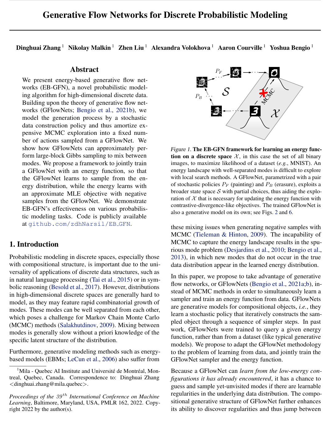
Here $\varnothing$ denotes an unassigned coordinate. Generation starts at $s_0=(\varnothing,\ldots,\varnothing)$ and terminates after exactly $D$ actions, each of which selects one unassigned coordinate and sets it to $0$ or $1$ . Thus, a terminal vector can be reached through many trajectories corresponding to different coordinate-ordering decisions. A forward policy $P_F(\cdot\mid s)$ assigns probabilities to the $2(D-|s|)$ possible assignments at state $s$ , where $|s|$ is the number of assigned coordinates. A backward policy $P_B(\cdot\mid s)$ assigns probabilities to the $|s|$ possible coordinate erasures.

The forward and backward policies are implemented with multilayer perceptrons. The input encodes $\varnothing$ as $-1$ and shares all hidden-layer weights between the two policies; only their final action-logit matrices differ. The scalar flow normalizer $Z$ is parameterized through $\log Z$ . This learned construction order allows the model to represent compositional regularities without imposing a fixed autoregressive ordering.
Knowl 2 — Trajectory-balance training of the GFlowNet
equation
For a complete trajectory $\tau=(s_0\to s_1\to\cdots\to s_n)$ ending at terminal state $s_n\in\mathcal{X}$ , the GFlowNet is trained with the squared trajectory-balance loss
$\mathcal{L}_\theta(\tau)=\left[\log\left(\frac{Z_\theta\prod_{t=0}^{n-1}P_F(s_{t+1}\mid s_t;\theta)}{R(s_n)\prod_{t=0}^{n-1}P_B(s_t\mid s_{t+1};\theta)}\right)\right]^2.$
Here $\theta$ denotes GFlowNet parameters, $R:\mathcal{X}\to\mathbb{R}_{\ge 0}$ is the terminal reward, $Z_\theta>0$ is the learned normalizing flow, and $P_F$ and $P_B$ are the forward and backward transition probabilities. The loss is evaluated on trajectories sampled either forward from $s_0$ or backward from a data example $x$ using $P_B$ .

If the loss is zero for every complete trajectory with positive reward, the terminal distribution induced by the forward policy satisfies $P_T(x)\propto R(x)$ , where $P_T(x)$ is the probability that forward sampling terminates at $x$ . Backward sampling from observed data is useful because it places training trajectories near data-supported regions that may be poorly visited by the current forward policy.
Knowl 3 — Alternating EB-GFN joint-training procedure
algorithm
EB-GFN jointly learns an energy function and a GFlowNet from a dataset $\{x_i\}$ without access to the normalized target distribution. The energy function $E_\phi(x)$ supplies the GFlowNet reward $R(x)=e^{-E_\phi(x)}$ , while the GFlowNet supplies negative samples for training $E_\phi$ .
Input: training dataset {x_i}, mixture coefficient α ∈ [0,1], GFlowNet parameters θ, energy parameters ϕ
Output: trained forward policy P_F, backward policy P_B, flow normalizer Z_θ, and energy E_ϕ
Initialize P_F, P_B, Z_θ, and E_ϕ
repeat
    Draw b ∼ Bernoulli(α)
    if b = 1 then
        Sample a complete trajectory τ forward from s_0 using P_F
    else
        Uniformly sample a data point x_i
        Sample a complete trajectory τ backward from x_i using P_B
    end if
    Update θ by a gradient step on the trajectory-balance loss using reward R(x)=e^{-E_ϕ(x)}
    Generate a negative terminal state x' with the GFlowNet-guided back-and-forth proposal
    Update ϕ using the gradient of E_ϕ(x)-E_ϕ(x') for a sampled data point x
until a convergence condition is reached
The paper uses $\alpha=1$ and $K=D$ for the Ising experiments, and $\alpha=0.5$ with $K$ increasing linearly from $1$ to $D$ for the synthetic and image experiments. The proposal-based energy update is performed once per energy update rather than iterating the proposal kernel to convergence. The method produces both a direct sampler, the trained forward GFlowNet, and an energy-based model.
Knowl 4 — Energy learning with GFlowNet-generated negative samples
equation
The energy model defines a distribution over the finite binary space $\mathcal{X}$ by
$p_\phi(x)=\frac{e^{-E_\phi(x)}}{Z_\phi},\qquad Z_\phi=\sum_{y\in\mathcal{X}}e^{-E_\phi(y)},$
where $E_\phi$ is the learned energy, $\phi$ its parameters, and $Z_\phi$ the intractable normalizer. The exact negative-log-likelihood gradient for a data point $x$ is
$-\nabla_\phi\log p_\phi(x)=\nabla_\phi E_\phi(x)-\mathbb{E}_{x'\sim p_\phi}\left[\nabla_\phi E_\phi(x')\right].$
EB-GFN replaces the intractable model expectation with terminal samples $x'\sim P_T$ , where $P_T$ is the distribution induced by the GFlowNet forward policy:
$\mathbb{E}_{x\sim p_{\mathrm{data}}}\left[\nabla_\phi E_\phi(x)\right]-\mathbb{E}_{x'\sim P_T}\left[\nabla_\phi E_\phi(x')\right].$
If the GFlowNet exactly matches the energy reward, so that $P_T(x)=p_\phi(x)$ , this update is an unbiased maximum-likelihood gradient for the energy model. During joint training, the GFlowNet therefore amortizes the negative-sample search that would otherwise require expensive MCMC.
Knowl 5 — GFlowNet back-and-forth Metropolis–Hastings proposal
algorithm
Given a terminal binary vector $x$ , an integer horizon $K$ with $1\le K\le D$ , and current policies $P_B$ and $P_F$ , EB-GFN constructs a large-block proposal as follows. First, sample $K$ erasures backward from $x=s_D$ to a partial state $s_{D-K}$ using $P_B$ . Then, starting from the same partial state, sample $K$ assignments forward using $P_F$ until reaching a proposed terminal vector $x'=s'_D$ .

The proposal changes at most $K$ coordinates. For the sampled backward path $\tau$ and forward path $\tau'$ , define
$P_B(\tau\mid x)=\prod_{t=D-K}^{D-1}P_B(s_t\mid s_{t+1}),\qquad P_F(\tau')=\prod_{t=D-K}^{D-1}P_F(s'_{t+1}\mid s'_t),$
with $s'_{D-K}=s_{D-K}$ . The reverse move from $x'$ to $x$ uses the reverse path probabilities $P_B(\tau'\mid x')$ and $P_F(\tau)$ . The proposal is accepted with probability
$A_{\tau,\tau'}(x\to x')=\min\left\{1,\frac{e^{-E_\phi(x')}\,P_B(\tau\mid x)P_F(\tau')}{e^{-E_\phi(x)}\,P_B(\tau'\mid x')P_F(\tau)}\right\}.$
If the proposal is rejected, the negative sample is set to $x$ ; otherwise it is $x'$ . Repeating this transition has the energy distribution proportional to $e^{-E_\phi(x)}$ as its stationary distribution. In EB-GFN training, one such transition is used to obtain each negative example, rather than running a long MCMC chain.
Knowl 6 — Perfect GFlowNet fitting eliminates proposal rejection
theoretical result
Suppose the GFlowNet satisfies the reward-matching condition for the energy reward $R(x)=e^{-E_\phi(x)}$ : the total trajectory flow terminating at every terminal state $x$ equals $R(x)$ . For any terminal state $x$ , any proposed terminal state $x'$ , and any pair of sampled backward and forward paths connecting them through a shared partial state, the path-probability ratio obeys
$e^{-E_\phi(x)}P_B(\tau\mid x)P_F(\tau')=e^{-E_\phi(x')}P_B(\tau'\mid x')P_F(\tau).$
Consequently, the Metropolis–Hastings acceptance probability for the GFlowNet back-and-forth proposal is exactly $1$ . The proposal therefore performs a rejection-free block update when the GFlowNet is perfectly trained. For $K=D$ , the shared partial state is the initial state $s_0$ , so the proposed terminal state is sampled directly from the GFlowNet forward policy and is independent of the starting terminal state. This is the paper's large-block Gibbs-sampling interpretation: unlike single-coordinate Gibbs updates, the learned proposal can change many coordinates and can jump between separated modes.
Knowl 7 — Uniform backward policy gives the maximum-entropy flow
theoretical result
For a Markovian flow $F$ on the partial-assignment DAG, define its forward-policy entropy as the expected sum of conditional entropies encountered along a complete trajectory:
$H[F]=\mathbb{E}_{\tau\sim P_F}\left[\sum_{t=0}^{n-1}H\big[P_F(\cdot\mid s_t)\big]\right],$
where $H[q]=-\sum_a q(a)\log q(a)$ for a discrete distribution $q$ . Fix any nonnegative terminal reward $R$ and consider all Markovian flows whose terminal flow equals $R(x)$ for every terminal state $x$ . The flow induced by choosing the backward policy uniformly over the parents of every state has maximal $H[F]$ among all such flows.

Thus, when several forward policies can realize the same terminal reward distribution, the canonical uniform-erasure backward policy selects the maximum-entropy solution. The result applies to the paper's $D$ -coordinate partial-assignment graph, where every trajectory passes through one state at each number of assigned coordinates.

Knowl 8 — Ising-model recovery and multimodal sampling

data/table

The paper tests EB-GFN on binary Ising models with spins $x\in\{-1,+1\}^{D}$ and energy

E_J(x)=-x^\top Jx,

where $J=\sigma A_N$ , $A_N$ is the adjacency matrix of an $N\times N$ toroidal grid, and $D=N^2$ . The model is trained only from 2000 samples and must recover a symmetric learned matrix $J_\phi$ . The metric is mean negative log-RMSE between $J$ and $J_\phi$ ; higher is better, and the reported standard deviation across runs is below $0.1$ .

Method and dimension	=0.1	0.2	0.3	0.4	0.5	-0.1	-0.2
Gibbs, D=10^2	4.8	4.7	3.4	2.6	2.3	4.8	4.7
GWG, D=10^2	4.8	4.7	3.4	2.6	2.3	4.8	4.7
EB-GFN, D=10^2	6.1	5.1	3.3	2.6	2.3	5.7	5.1
Gibbs, D=9^2	–	–	–	–	–	4.8	4.7
GWG, D=9^2	–	–	–	–	–	4.8	4.7
EB-GFN, D=9^2	–	–	–	–	–	5.7	5.1

For positive $\sigma$ , the learned samples show contiguous same-spin regions; for negative $\sigma$ , they show checkerboard-like modes. The visualizations on page 6 show that EB-GFN nearly reconstructs the full interaction graph despite receiving no grid-structure information. Its clearest advantage occurs for the negative- $\sigma$ multimodal cases, where local Gibbs-style methods must move between separated checkerboard modes.

Knowl 9 — Synthetic discrete-density modeling results

data/table

The synthetic benchmark converts seven planar distributions—2spirals, 8gaussians, circles, moons, pinwheel, swissroll, and checkerboard—into 32-bit binary vectors. Each planar coordinate is quantized into $2^{16}$ buckets and represented by a 16-bit Gray code, so neighboring planar buckets differ by one bit. EB-GFN uses $\alpha=0.5$ and increases the back-and-forth horizon $K$ linearly from $1$ to $D=32$ . It is compared with PCD, ALOE, and the much larger ALOE+ model. Lower NLL and MMD are better; MMD values are in units of $1\times10^{-4}$ .

NLL	2spirals	8gaussians	circles	moons	pinwheel	swissroll	checkerboard
PCD	20.094	19.991	20.565	19.763	19.593	20.172	21.214
ALOE	20.295	20.350	20.565	19.287	19.821	20.160	54.653
ALOE+	20.062	19.984	20.570	19.743	19.576	20.170	21.142
EB-GFN	20.050	19.982	20.546	19.732	19.554	20.146	20.696
MMD	2spirals	8gaussians	circles	moons	pinwheel	swissroll	checkerboard
PCD	2.160	0.954	0.188	0.962	0.505	1.382	2.831
ALOE	21.926	107.320	0.497	26.894	39.091	0.471	61.562
ALOE+	0.149	0.078	0.636	0.516	1.746	0.718	12.138
EB-GFN	0.583	0.531	0.305	0.121	0.492	0.274	1.206

EB-GFN has the lowest reported NLL on all seven distributions. Its MMD is particularly strong on moons, pinwheel, swissroll, and checkerboard; ALOE+ is better on 2spirals and 8gaussians, while PCD has a lower raw MMD value on circles. The page-7 visualizations show that EB-GFN recovers multimodal energy landscapes and generated samples, especially for checkerboard and 8gaussians, without the roughly thirty-times-larger parametrization used by ALOE+.

Knowl 10 — Discrete image modeling performance

data/table

The image experiments train multilayer-perceptron energy models on four binary image datasets using PCD-100-style training with replay buffers, comparing Gibbs, Gibbs-With-Gradients (GWG), and EB-GFN. EB-GFN uses a three-hidden-layer, 512-unit GFlowNet, a three-hidden-layer, 256-unit energy MLP, an equal mixture of forward and data-conditioned backward trajectories, and a horizon $K$ increased linearly from $1$ to the image dimension. The reported metric is test negative log-likelihood per sample, so lower is better.

EB-GFN improves on GWG for Omniglot, Silhouettes, and Dynamic MNIST, but not Static MNIST. The page-8 Dynamic MNIST visualizations show that EB-GFN captures some mode details more faithfully than the baselines. Adding LayerNorm to every forward-policy linear layer except the last further reduces EB-GFN NLL from $112.59$ to $104.88$ on Omniglot, from $185.57$ to $174.48$ on Silhouettes, from $102.43$ to $89.48$ on Static MNIST, and from $105.75$ to $88.76$ on Dynamic MNIST.

Coverage note — The importance-sampling estimator for evaluating GFlowNet likelihoods and the detailed backward-policy visualizations were omitted because they are auxiliary evaluation and diagnostic material; the core proposal, theory, training procedure, and benchmark results are included.

References

1.Arbel, M., Zhou, L., and Gretton, A. Generalized energy based models. International Conference on Learning Representations (ICLR), 2021.
2.Ba, J., Kiros, J. R., and Hinton, G. E. Layer normalization. ArXiv, abs/1607.06450, 2016.
3.Bengio, E., Pineau, J., and Precup, D. Interference and generalization in temporal difference learning. International Conference on Machine Learning (ICML), 2020.
4.Bengio, E., Jain, M., Korablyov, M., Precup, D., and Bengio, Y. Flow network based generative models for non-iterative diverse candidate generation. Neural Information Processing Systems (NeurIPS), 2021a.
5.Bengio, Y., Mesnil, G., Dauphin, Y., and Rifai, S. Better mixing via deep representations. International Conference on Machine Learning (ICML), 2013.
6.Bengio, Y., Deleu, T., Hu, E., Lahlou, S., Tiwari, M., and Bengio, E. GFlowNet foundations. arXiv preprint 2111.09266, 2021b.
7.Besold, T. R., d’Avila Garcez, A. S., Bader, S., Bowman, H., Domingos, P. M., Hitzler, P., Kuhnberger, K.-U., Lamb, L., Lowd, D., Lima, P. M. V., de Penning, L., Pinkas, G., Poon, H., and Zaverucha, G. Neural-symbolic learning and reasoning: A survey and interpretation. arXiv preprint 1711.03902, 2017.
8.Clevert, D.-A., Unterthiner, T., and Hochreiter, S. Fast and accurate deep network learning by exponential linear units (ELUs). International Conference on Learning Representations (ICLR), 2016.
9.Dai, B., Liu, Z., Dai, H., He, N., Gretton, A., Song, L., and Schuurmans, D. Exponential family estimation via adversarial dynamics embedding. Neural Information Processing Systems (NeurIPS), 2019.
10.Dai, H., Singh, R., Dai, B., Sutton, C., and Schuurmans, D. Learning discrete energy-based models via auxiliary-variable local exploration. Neural Information Processing Systems (NeurIPS), 2020.
11.Desjardins, G., Courville, A. C., Bengio, Y., Vincent, P., and Delalleau, O. Tempered Markov chain Monte Carlo for training of restricted Boltzmann machines. Artificial Intelligence and Statistics (AISTATS), 2010.
12.Du, Y. and Mordatch, I. Implicit generation and generalization in energy-based models. Neural Information Processing Systems (NeurIPS), 2019.
13.Du, Y., Li, S., Tenenbaum, J. B., and Mordatch, I. Improved contrastive divergence training of energy based models. International Conference on Machine Learning (ICML), 2021.
14.Emelianenko, D., Voita, E., and Serdyukov, P. Sequence modeling with unconstrained generation order. Neural Information Processing Systems (NeurIPS), 2019.
15.Ford, L. R. and Fulkerson, D. R. Maximal flow through a network. Canadian Journal of Mathematics, 8:243–248, 1956.
16.Gao, R., Song, Y., Poole, B., Wu, Y. N., and Kingma, D. P. Learning energy-based models by diffusion recovery likelihood. International Conference on Learning Representations (ICLR), 2021.
17.Germain, M., Gregor, K., Murray, I., and Larochelle, H. MADE: Masked autoencoder for distribution estimation. International Conference on Machine Learning (ICML), 2015.
18.Grathwohl, W., Chen, R. T. Q., Bettencourt, J., Sutskever, I., and Duvenaud, D. K. Ffjord: Free-form continuous dynamics for scalable reversible generative models. International Conference on Learning Representations (ICLR), 2019.
19.Grathwohl, W., Kelly, J., Hashemi, M., Norouzi, M., Swersky, K., and Duvenaud, D. K. No MCMC for me: Amortized sampling for fast and stable training of energy-based models. International Conference on Learning Representations (ICLR), 2021a.
20.Grathwohl, W., Swersky, K., Hashemi, M., Duvenaud, D. K., and Maddison, C. J. Oops I took a gradient: Scalable sampling for discrete distributions. International Conference on Machine Learning (ICML), 2021b.
21.Graves, A. Generating sequences with recurrent neural networks. arXiv preprint 1308.0850, 2013.
22.Gray, F. Pulse code communication. US Patent 2,632,058, 1953.
23.Gretton, A., Borgwardt, K. M., Rasch, M. J., Scholkopf, B., and Smola, A. A kernel two-sample test. J. Mach. Learn. Res., 13:723–773, 2012.
24.Haarnoja, T., Tang, H., Abbeel, P., and Levine, S. Reinforcement learning with deep energy-based policies. International Conference on Machine Learning (ICML), 2017.
25.Han, J., Ding, F., Liu, X., Torresani, L., Peng, J., and Liu, Q. Stein variational inference for discrete distributions. Artificial Intelligence and Statistics (AISTATS), 2020.
26.Hastings, W. K. Monte Carlo sampling methods using Markov chains and their applications. Biometrika, 57(1):97–109, 1970.
27.Hinton, G. E. Training products of experts by minimizing contrastive divergence. Neural Computation, 14:1771–1800, 2002.
28.Hinton, G. E., Osindero, S., and Teh, Y. W. A fast learning algorithm for deep belief nets. Neural Computation, 18:1527–1554, 2006.
29.Ising, E. Beitrag zur Theorie des Ferromagnetismus. Zeitschrift fur Physik, 31(1):253–258, 1925.
30.Jain, M., Bengio, E., Garc´ıa, A., Rector-Brooks, J., Dossou, B. F. P., Ekbote, C. A., Fu, J., Zhang, T., Kilgour, M., Zhang, D., Simine, L., Das, P., and Bengio, Y. Biological sequence design with gflownets. ArXiv, abs/2203.04115, 2022.
31.LeCun, Y., Chopra, S., Hadsell, R., Ranzato, A., and Huang, F. J. A tutorial on energy-based learning. 2006.
32.Li, X., Trabucco, B., Park, D., Luo, M., Shen, S. M., Darrell, T., and Gao, Y. Discovering non-monotonic autoregressive orderings with variational inference. International Conference on Learning Representations (ICLR), 2021.
33.Ma, Y., Ma, Y.-A., Chen, T., and Fox, E. B. A complete recipe for stochastic gradient MCMC. Neural Information Processing Systems (NIPS), 2015.
34.MacKay, D. J. C. Information Theory, Inference, and Learning Algorithms. Cambridge University Press, 2003.
35.Malkin, N., Jain, M., Bengio, E., Sun, C., and Bengio, Y. Trajectory balance: Improved credit assignment in GFlowNets. arXiv preprint 2201.13259, 2022.
36.Meng, C., Song, J., Song, Y., Zhao, S., and Ermon, S. Improved autoregressive modeling with distribution smoothing. International Conference on Learning Representations (ICLR), 2021.
37.Nijkamp, E., Hill, M., Zhu, S.-C., and Wu, Y. N. Learning non-convergent non-persistent short-run mcmc toward energy-based model. Neural Information Processing Systems (NeurIPS), 2019.
38.Nijkamp, E., Hill, M., Han, T., Zhu, S.-C., and Wu, Y. N. On the anatomy of MCMC-based maximum likelihood learning of energy-based models. Association for the Advancement of Artificial Intelligence (AAAI), 2020.
39.Salakhutdinov, R. Learning in Markov random fields using tempered transitions. Neural Information Processing Systems (NIPS), 2009.
40.Salakhutdinov, R. and Hinton, G. E. Deep Boltzmann machines. Artificial Intelligence and Statistics (AISTATS), 2009.
41.Song, Y. and Kingma, D. P. How to train your energy-based models. arXiv preprint 2101.03288, 2021.
42.Sutskever, I., Martens, J., and Hinton, G. E. Generating text with recurrent neural networks. International Conference on Machine Learning (ICML), 2011.
43.Sutton, R. S. Learning to predict by the methods of temporal differences. Machine Learning, 3:9–44, 2005.
44.Sutton, R. S. and Barto, A. G. Reinforcement learning: An introduction. IEEE Transactions on Neural Networks, 16:285–286, 2005.
45.Tai, K. S., Socher, R., and Manning, C. D. Improved semantic representations from tree-structured long short-term memory networks. Association for Computational Linguistics (ACL), 2015.
46.Tieleman, T. Training restricted Boltzmann machines using approximations to the likelihood gradient. International Conference on Machine Learning (ICML), 2008.
47.Tieleman, T. and Hinton, G. E. Using fast weights to improve persistent contrastive divergence. International Conference on Machine Learning (ICML), 2009.
48.Titsias, M. K. and Yau, C. The hamming ball sampler. Journal of the American Statistical Association, 112:1598 – 1611, 2017.
49.Uria, B., Cotˆ e, M.-A., Gregor, K., Murray, I., and Larochelle, H. Neural autoregressive distribution estimation. Journal of Machine Learning Research, 17:205:1–205:37, 2016.
50.van den Oord, A., Kalchbrenner, N., Espeholt, L., Kavukcuoglu, K., Vinyals, O., and Graves, A. Conditional image generation with pixelcnn decoders. Neural Information Processing Systems (NIPS), 2016a.
51.van den Oord, A., Kalchbrenner, N., and Kavukcuoglu, K. Pixel recurrent neural networks. International Conference on Machine Learning (ICML), 2016b.
52.Wang, J.-S. and Swendsen, R. H. Cluster Monte Carlo algorithms. Physica A: Statistical Mechanics and its Applications, 167(3):565–579, 1990.
53.Welling, M. and Teh, Y. W. Bayesian learning via stochastic gradient Langevin dynamics. International Conference on Machine Learning (ICML), 2011.
54.Xie, J., Lu, Y., Zhu, S.-C., and Wu, Y. N. A theory of generative convnet. ArXiv, abs/1602.03264, 2016.
55.Yu, L., Song, Y., Song, J., and Ermon, S. Training deep energy-based models with f-divergence minimization. International Conference on Machine Learning (ICML), 2020.
56.Zanella, G. Informed proposals for local mcmc in discrete spaces. Journal of the American Statistical Association, 115:852 – 865, 2019.
57.Zhang, R., Liu, X., and Liu, Q. A langevin-like sampler for discrete distributions. In International Conference on Machine Learning. PMLR, 2022.

Citation

MLA

Zhang, D., et al. “Generative Flow Networks for Discrete Probabilistic Modeling”. International Conference on Machine Learning, vol. 162, 2022, pp. 26412–28, https://proceedings.mlr.press/v162/zhang22v.html.

APA

Zhang, D., Malkin, N., Liu, Z., Volokhova, A., Courville, A., & Bengio, Y. (2022). Generative Flow Networks for Discrete Probabilistic Modeling. International Conference on Machine Learning, 162, 26412–26428. https://proceedings.mlr.press/v162/zhang22v.html

Chicago

Zhang, D., N. Malkin, Z. Liu, A. Volokhova, A. Courville, and Y. Bengio. 2022. “Generative Flow Networks for Discrete Probabilistic Modeling”. International Conference on Machine Learning 162: 26412–28. https://proceedings.mlr.press/v162/zhang22v.html.

Harvard

Zhang, D. et al. (2022) “Generative Flow Networks for Discrete Probabilistic Modeling”, International Conference on Machine Learning. PMLR, pp. 26412–26428. Available at: https://proceedings.mlr.press/v162/zhang22v.html.

Vancouver

1. Zhang D, Malkin N, Liu Z, Volokhova A, Courville A, Bengio Y (2022) Generative Flow Networks for Discrete Probabilistic Modeling. In: International Conference on Machine Learning. PMLR, pp 26412–26428

BibTeX

@InProceedings{pmlr-v162-zhang22v,
  title = 	 {Generative Flow Networks for Discrete Probabilistic Modeling},
  author =       {Zhang, Dinghuai and Malkin, Nikolay and Liu, Zhen and Volokhova, Alexandra and Courville, Aaron and Bengio, Yoshua},
  booktitle = 	 {Proceedings of the 39th International Conference on Machine Learning},
  pages = 	 {26412--26428},
  year = 	 {2022},
  editor = 	 {Chaudhuri, Kamalika and Jegelka, Stefanie and Song, Le and Szepesvari, Csaba and Niu, Gang and Sabato, Sivan},
  volume = 	 {162},
  series = 	 {Proceedings of Machine Learning Research},
  month = 	 {17--23 Jul},
  publisher =    {PMLR},
  pdf = 	 {https://proceedings.mlr.press/v162/zhang22v/zhang22v.pdf},
  url = 	 {https://proceedings.mlr.press/v162/zhang22v.html},
  abstract = 	 {We present energy-based generative flow networks (EB-GFN), a novel probabilistic modeling algorithm for high-dimensional discrete data. Building upon the theory of generative flow networks (GFlowNets), we model the generation process by a stochastic data construction policy and thus amortize expensive MCMC exploration into a fixed number of actions sampled from a GFlowNet. We show how GFlowNets can approximately perform large-block Gibbs sampling to mix between modes. We propose a framework to jointly train a GFlowNet with an energy function, so that the GFlowNet learns to sample from the energy distribution, while the energy learns with an approximate MLE objective with negative samples from the GFlowNet. We demonstrate EB-GFN’s effectiveness on various probabilistic modeling tasks. Code is publicly available at https://github.com/zdhNarsil/EB_GFN.}
}

Metadata:DOI registry

Access the Paper

This paper is available from its original source. Click below to access the PDF.

Open PDF

License: https://creativecommons.org/licenses/by/4.0/

Dataset	Gibbs	GWG	EB-GFN
Omniglot	133.92	114.96	112.59
Silhouettes	475.55	188.82	185.57
Static MNIST	173.61	99.36	102.43
Dynamic MNIST	162.25	108.29	105.75

Generative Flow Networks for Discrete Probabilistic Modeling

Abstract

Topics

Keywords

Table of Contents

Knowls

Knowl 1 — Non-autoregressive discrete GFlowNet construction

Knowl 2 — Trajectory-balance training of the GFlowNet

Knowl 3 — Alternating EB-GFN joint-training procedure

Knowl 4 — Energy learning with GFlowNet-generated negative samples

Knowl 5 — GFlowNet back-and-forth Metropolis–Hastings proposal

Knowl 6 — Perfect GFlowNet fitting eliminates proposal rejection

Knowl 7 — Uniform backward policy gives the maximum-entropy flow

Knowl 8 — Ising-model recovery and multimodal sampling

Knowl 9 — Synthetic discrete-density modeling results

Knowl 10 — Discrete image modeling performance

References

Citation

BibTeX

Access the Paper