GFlowNet Foundations

Yoshua BengioSalem LahlouTristan DeleuEdward J. HuMo TiwariEmmanuel Bengio

article2023JMLR378 citations

Establishes the theoretical foundations of Generative Flow Networks by introducing the detailed balance training objective and showing how they amortize complex Markov chain Monte Carlo sampling and marginalization over composite structures like graphs and sets in a single generative pass.

Listen

Generating diverse, high-quality candidates across complex discrete spaces—such as molecular structures, genetic sequences, and causal networks—presents a major bottleneck in scientific discovery and probabilistic inference. Traditional sampling methods like Markov Chain Monte Carlo often struggle because they require lengthy, sequential chains that become trapped in local probability modes. Conversely, standard reinforcement learning techniques generally concentrate on finding a single best outcome rather than exploring a broad distribution of viable candidates.

The article establishes a rigorous theoretical foundation for Generative Flow Networks (GFlowNets) and evaluates their ability to serve as efficient, amortized generative samplers. It aims to demonstrate how GFlowNets can accurately learn to sample compositional objects with probabilities proportional to a specified reward function while also computing complex marginal probabilities, free energies, and information-theoretic quantities.

The authors develop mathematical proofs based on network flow theory on directed acyclic graphs, mapping generative construction trajectories to probability measures. They evaluate learning properties using local training objectives, including a proposed detailed-balance formulation that enforces flow conservation without requiring explicit sums over all possible transitions. The approach also reviews implementations across structured combinatorial domains, such as sets, graphs, and active learning pipelines.

The analysis yields four key findings. First, GFlowNets amortize the cost of inference: paying an upfront computational training cost enables rapid, single-pass generation of independent samples, bypassing the mode-mixing issues common in iterative sampling. Second, the detailed-balance objective provides an efficient local training mechanism that decouples forward generation from backward trajectory preferences. Third, conditional GFlowNets can calculate otherwise intractable marginal distributions, enabling direct estimation of partition functions, free energies, entropies, and mutual information. Fourth, unlike maximum entropy reinforcement learning—which unintentionally over-samples states that have exponentially more construction paths—GFlowNets maintain sampling probabilities that remain strictly proportional to the specified target reward.

These findings mean that organizations engaged in computational biology, drug discovery, hardware design, and latent variable modeling can reduce exploration cycle times and avoid missing viable candidates across high-dimensional design spaces. In active learning setups with costly experimental evaluations, GFlowNets provide the candidate diversity needed to explore uncertain regions effectively and mitigate proxy model misspecification.

Decision-makers should evaluate GFlowNets for candidate-generation and active learning pipelines where target spaces possess latent, generalizable structure and where generating diverse batches is critical. For exploratory or modular problems, teams should adopt detailed-balance or trajectory-balance training objectives and test joint architectures that update reward proxies alongside the generative policy.

Users should note that GFlowNets rely on the neural network's capacity to generalize across structured reward landscapes; if the target reward landscape lacks underlying structure, the training problem becomes intractable in high dimensions. In addition, while the foundational theory is mathematically rigorous, scaling continuous-space and hierarchical implementations into production environments will require careful empirical validation and parameter tuning.

CIFAR IVADO McGill University Microsoft Mila Stanford University Université de Montréal active learning conditional probabilities marginals GFlowNet framework conditional GFlowNet flow-matching loss

arXiv: 2111.09266

Paper: Normalizing Flows for Probabilistic Modeling and Inference, George Papamakarios et al. (2019). Provides a comprehensive foundation in continuous flow-based generative modeling and density estimation that clarifies the theoretical shift to flow networks on discrete DAGs.
Paper: Variational Inference with Normalizing Flows, Danilo Jimenez Rezende et al. (2015). Introduces variational inference with normalizing flows, establishing the core principles of amortized inference and expressive density modeling foundational to GFlowNets.
Paper: DAGs with NO TEARS: Continuous Optimization for Structure Learning, Xun Zheng et al. (2018). Formulates continuous optimization and graph learning over directed acyclic graphs, providing essential context for GFlowNets' structure-generation and DAG-based flows.
Paper: Categorical Reparameterization with Gumbel-Softmax, Eric Jang et al. (2017). Presents categorical reparameterization techniques for discrete generative modeling, establishing key background on navigating discrete and combinatorial sample spaces.

Paper: Joint Bayesian Inference of Graphical Structure and Parameters with a Single Generative Flow Network, Tristan Deleu et al. (2023). Directly applies and extends the GFlowNet theoretical framework to perform joint Bayesian posterior inference over both Bayesian network graph structures and continuous parameters.
Paper: Local Search GFlowNets, Minsu Kim et al. (2024). Builds upon foundational GFlowNet training objectives by incorporating local search to mitigate over-exploration and improve sample efficiency in high-reward discrete spaces.

Abstract

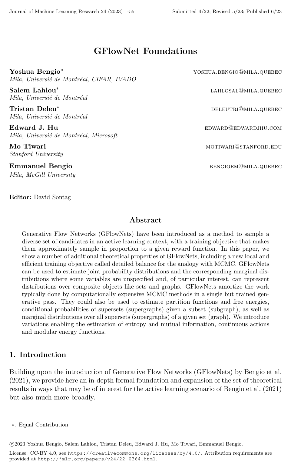
Generative Flow Networks (GFlowNets) have been introduced as a method to sample a diverse set of candidates in an active learning context, with a training objective that makes them approximately sample in proportion to a given reward function. In this paper, we show a number of additional theoretical properties of GFlowNets, including a new local and efficient training objective called detailed balance for the analogy with MCMC. GFlowNets can be used to estimate joint probability distributions and the corresponding marginal distributions where some variables are unspecified and, of particular interest, can represent distributions over composite objects like sets and graphs. GFlowNets amortize the work typically done by computationally expensive MCMC methods in a single but trained generative pass. They could also be used to estimate partition functions and free energies, conditional probabilities of supersets (supergraphs) given a subset (subgraph), as well as marginal distributions over all supersets (supergraphs) of a given set (graph). We introduce variations enabling the estimation of entropy and mutual information, continuous actions and modular energy functions.

Topics

active learning conditional probabilities marginals mcmc mcmc method mutual informations reward function distribution functions bipartite graphs random variables

Keywords

GFlowNet framework conditional GFlowNet flow-matching loss trajectory flow Markovian flows flow parametrization generative policy Monte-Carlo Markov chains

1. Introduction
1.1 What is a GFlowNet ?
1.2 Contributions of this paper
1.3 GFlowNets in other works
2. Flow Networks and Markovian Flows
2.1 Some elements of graph theory
2.2 Trajectories and Flows
2.3 Flow Induced Probability Measures
2.4 Markovian Flows
2.5 Flow Matching Conditions
2.6 Backwards Transitions can be Chosen Freely
2.7 Equivalence Between Flows
3. GFlowNets: Learning a Flow
3.1 GFlowNets as an Alternative to MCMC Sampling
3.2 GFlowNets and flow-matching losses
3.3 Extensions
3.3.1 Introducing Time Stamps to Allow Cycles
3.3.2 Stochastic Rewards
3.3.3 GFlowNets can be trained offline
3.4 Exploiting Data as Known Terminating States
4. Conditional Flows and Free energies
4.1 Conditional flow networks
4.2 Reward-conditional flow networks
4.3 State-conditional flow networks
4.4 Conditional GFlowNets
4.5 Training Energy-Based Models with a GFlowNet
4.6 Active Learning with a GFlowNet
4.7 Estimating Entropies, Conditional Entropies and Mutual Information
5. GFlowNets on Sets, Graphs, and to Marginalize Joint Distributions
5.1 Set GFlowNets
5.2 GFlowNet on Graphs
5.3 Marginalizing over Missing Variables
5.4 Modular Energy Function Decomposition
6. Continuous or Hybrid Actions and States
6.1 Integrable Normalization Constants
6.2 GFlowNets in GFlowNets
7. Related Work
7.1 Contrast with Generative Models
7.2 Contrast with Regularized Reinforcement Learning
7.3 Contrast with Monte-Carlo Markov Chain methods
8. Conclusions and Open Questions
Acknowledgements
References

Knowls

Knowl 1 — Pointed DAG Formulation of Flow Networks and Terminating State Probabilities
definition
Let $G = (\mathcal{S}, \mathbb{A})$ be a directed acyclic graph (DAG) with a finite state set $\mathcal{S}$ and directed transitions $\mathbb{A} \subseteq \mathcal{S} \times \mathcal{S}$ . $G$ is a pointed DAG if it contains a unique source state $s_0$ and a unique sink state $s_f$ such that for all $s \in \mathcal{S} \setminus \{s_0, s_f\}$ , $s_0 < s < s_f$ , where $<$ denotes the reachability strict partial order.

A complete trajectory is a path $\tau = (s_0, s_1, \dots, s_n, s_{n+1}=s_f)$ with each $(s_t \to s_{t+1}) \in \mathbb{A}$ . The set of all complete trajectories is denoted $\mathcal{T}$ . A terminating state $s \in \mathcal{S}^f$ is any parent of $s_f$ (i.e., $(s \to s_f) \in \mathbb{A}$ ), and $(s \to s_f)$ is termed a terminating edge.

A trajectory flow is a non-negative function $F: \mathcal{T} \to \mathbb{R}^+$ inducing a measure over $\mathcal{T}$ . It defines:
- State flow: $F(s) = \sum_{\tau \in \mathcal{T} : s \in \tau} F(\tau)$
- Edge flow: $F(s \to s') = \sum_{\tau \in \mathcal{T} : (s \to s') \in \tau} F(\tau)$
- Total flow (partition function): $Z = F(s_0) = F(s_f) = \sum_{\tau \in \mathcal{T}} F(\tau)$
- Forward and backward transition probabilities for $(s \to s') \in \mathbb{A}$ : $P_F(s' \mid s) = \frac{F(s \to s')}{F(s)}, \quad P_B(s \mid s') = \frac{F(s \to s')}{F(s')}$
- Terminating state probability distribution over $s \in \mathcal{S}^f$ : $P_T(s) = P(s \to s_f) = \frac{F(s \to s_f)}{Z}$
When a GFlowNet is trained to match a target non-negative reward function $R: \mathcal{S}^f \to \mathbb{R}^+$ such that $F(s \to s_f) = R(s)$ , the terminating state sampling distribution satisfies $P_T(s) = \frac{R(s)}{Z} \propto R(s)$ .
Knowl 2 — Characterization and Unique Parametrization of Markovian Flows
theoretical result
In a flow network $(G, F)$ over a pointed DAG $G = (\mathcal{S}, \mathbb{A})$ , the flow $F$ is defined to be Markovian if for any state $s \neq s_0$ , outgoing edge $s \to s'$ , and partial trajectory $\tau = (s_0, s_1, \dots, s_n = s)$ , the conditional transition probability satisfies: $P(s \to s' \mid \tau) = P(s \to s' \mid s) = P_F(s' \mid s)$

For any flow network $(G, F)$ with flow probability measure $P$ , the following three conditions are equivalent:
1. $F$ is a Markovian flow.
2. The probability of any complete trajectory $\tau = (s_0, s_1, \dots, s_n, s_{n+1} = s_f)$ factorizes via forward transition probabilities: $P(\tau) = \prod_{t=1}^{n+1} P_F(s_t \mid s_{t-1})$
3. The probability of any complete trajectory factorizes via backward transition probabilities: $P(\tau) = \prod_{t=1}^{n+1} P_B(s_{t-1} \mid s_t)$
As a consequence, a Markovian flow on a pointed DAG is uniquely determined by any one of the following specifications:
1. The total flow $\hat{Z}$ and the forward transition probabilities $\hat{P}_F(s' \mid s)$ for all edges $(s \to s') \in \mathbb{A}$ .
2. The total flow $\hat{Z}$ and the backward transition probabilities $\hat{P}_B(s \mid s')$ for all edges $(s \to s') \in \mathbb{A}$ .
3. The terminating flows $\hat{F}(s \to s_f)$ for all terminating edges $(s \to s_f) \in \mathbb{A}^f$ together with the backward transition probabilities $\hat{P}_B(s \mid s')$ for all non-terminating edges $(s \to s') \in \mathbb{A} \setminus \mathbb{A}^f$ .
Moreover, two flows $F_1, F_2$ are defined as equivalent if they coincide on all edge flows. For every general trajectory flow $F'$ , there exists a unique equivalent Markovian flow $F$ .
Knowl 3 — Detailed Balance Condition and Detailed Balance Loss for GFlowNets
theoretical result
Let $G = (\mathcal{S}, \mathbb{A})$ be a pointed DAG. A non-negative state flow function $\hat{F}: \mathcal{S} \to \mathbb{R}^+$ , forward transition probability function $\hat{P}_F$ , and backward transition probability function $\hat{P}_B$ jointly correspond to a valid Markovian flow if and only if they satisfy the detailed balance condition on every transition $(s \to s') \in \mathbb{A}$ : $\hat{F}(s) \hat{P}_F(s' \mid s) = \hat{F}(s') \hat{P}_B(s \mid s')$

Given a target reward function $R: \mathcal{S}^f \to \mathbb{R}^+$ for terminating states $s \in \mathcal{S}^f$ (with terminating transition $s \to s_f$ and boundary condition $\hat{F}(s_f) = R(s)$ ), the edge-decomposable Detailed Balance loss $\mathcal{L}_{\mathrm{DB}}$ on a single edge $(s \to s') \in \mathbb{A}$ with hyperparameter $\delta \ge 0$ is defined as: $\mathcal{L}_{\mathrm{DB}}(\hat{F}, \hat{P}_F, \hat{P}_B, s \to s') = \begin{cases} \left( \log \frac{\delta + \hat{F}(s)\hat{P}_F(s' \mid s)}{\delta + \hat{F}(s')\hat{P}_B(s \mid s')} \right)^2 & \text{if } s' \neq s_f, \\ \left( \log \frac{\delta + \hat{F}(s)\hat{P}_F(s' \mid s)}{\delta + R(s)} \right)^2 & \text{if } s' = s_f \end{cases}$

The total detailed balance loss $\mathcal{L}_{\mathrm{DB}}(\hat{F}, \hat{P}_F, \hat{P}_B) = \sum_{(s \to s') \in \mathbb{A}} \mathcal{L}_{\mathrm{DB}}(\hat{F}, \hat{P}_F, \hat{P}_B, s \to s')$ equals zero if and only if $(\hat{F}, \hat{P}_F, \hat{P}_B)$ corresponds to a valid Markovian flow matching the target reward. Unlike flow matching, this condition is purely local and avoids explicit summations over parent or child sets.
Knowl 4 — Flow Matching Conditions and Flow Matching Loss
theoretical result
Let $G = (\mathcal{S}, \mathbb{A})$ be a pointed DAG with source state $s_0$ and sink state $s_f$ . A non-negative function $\hat{F}$ defined on states $\mathcal{S}$ and transitions $\mathbb{A}$ defines a valid flow if and only if it satisfies the flow matching conditions for all internal states: $\forall s' > s_0, \quad \hat{F}(s') = \sum_{s \in \mathrm{Par}(s')} \hat{F}(s \to s')$ $\forall s' < s_f, \quad \hat{F}(s') = \sum_{s'' \in \mathrm{Child}(s')} \hat{F}(s' \to s'')$ where $\mathrm{Par}(s') = \{s \in \mathcal{S} : (s \to s') \in \mathbb{A}\}$ and $\mathrm{Child}(s') = \{s'' \in \mathcal{S} : (s' \to s'') \in \mathbb{A}\}$ . When satisfied, $\hat{F}$ uniquely defines a Markovian flow $F$ over complete trajectories $\tau = (s_0, s_1, \dots, s_n, s_{n+1} = s_f)$ : $F(\tau) = \frac{\prod_{t=1}^{n+1} \hat{F}(s_{t-1} \to s_t)}{\prod_{t=1}^n \hat{F}(s_t)}$

For an edge-flow parametrization with reward $R(s) = \hat{F}(s \to s_f)$ , the state-decomposable Flow Matching loss $\mathcal{L}_{\mathrm{FM}}$ for a state $s' \in \mathcal{S} \setminus \{s_f\}$ with smoothing parameter $\delta \ge 0$ is: $\mathcal{L}_{\mathrm{FM}}(\hat{F}, s') = \left( \log \frac{\delta + \sum_{s \in \mathrm{Par}(s')} \hat{F}(s \to s')}{\delta + R(s')\mathbf{1}_{s' \in \mathcal{S}^f} + \sum_{s'' \in \mathrm{Child}(s') \setminus \{s_f\}} \hat{F}(s' \to s'')} \right)^2$ The total loss $\mathcal{L}_{\mathrm{FM}}(\hat{F}) = \sum_{s \in \mathcal{S}} \mathcal{L}_{\mathrm{FM}}(\hat{F}, s)$ attains zero if and only if $\hat{F}$ defines a valid Markovian flow matching the target rewards.
Knowl 5 — Trajectory Balance Loss Formulation
model/method
The trajectory balance objective parametrizes a GFlowNet on a pointed DAG $G = (\mathcal{S}, \mathbb{A})$ with target terminal reward $R: \mathcal{S}^f \to \mathbb{R}^+$ using a learned scalar partition function $\hat{Z} \in \mathbb{R}^+$ , forward transition probabilities $\hat{P}_F(s_{t+1} \mid s_t)$ , and backward transition probabilities $\hat{P}_B(s_t \mid s_{t+1})$ .

For any complete trajectory $\tau = (s_0, s_1, \dots, s_n, s_{n+1} = s_f) \in \mathcal{T}$ terminating at state $s_n \in \mathcal{S}^f$ , the trajectory balance loss $\mathcal{L}_{\mathrm{TB}}$ is: $\mathcal{L}_{\mathrm{TB}}(\hat{Z}, \hat{P}_F, \hat{P}_B, \tau) = \left( \log \frac{\hat{Z} \prod_{t=1}^{n+1} \hat{P}_F(s_t \mid s_{t-1})}{R(s_n) \prod_{t=1}^n \hat{P}_B(s_{t-1} \mid s_t)} \right)^2$ where $\hat{P}_F(s_f \mid s_n) = 1$ and the backward transition probability product runs over internal edges $t=1, \dots, n$ .

The total loss $\mathcal{L}_{\mathrm{TB}}(\hat{Z}, \hat{P}_F, \hat{P}_B) = \sum_{\tau \in \mathcal{T}} \mathcal{L}_{\mathrm{TB}}(\hat{Z}, \hat{P}_F, \hat{P}_B, \tau)$ is trajectory-decomposable, and any global minimizer where $\mathcal{L}_{\mathrm{TB}} = 0$ corresponds to a valid Markovian flow with exact partition function $\hat{Z} = Z$ and terminating state distribution $P_T(s) = R(s)/Z$ .
Knowl 6 — State-Conditional Flow Networks and Free Energy Computation
theoretical result
Given a pointed DAG $G = (\mathcal{S}, \mathbb{A})$ with energy function $\mathcal{E}: \mathcal{S} \to \mathbb{R}$ and terminating edge flows $F(s' \to s_f) = e^{-\mathcal{E}(s')}$ , the free energy $\mathcal{F}(s)$ of an internal state $s \in \mathcal{S}$ is defined as: $e^{-\mathcal{F}(s)} = \sum_{s' : s' \ge s} e^{-\mathcal{E}(s')}$ where $\ge$ is the reachability partial order in $G$ .

For any state $s \in \mathcal{S}$ , let $G_s$ be the subgraph of $G$ containing all descendant states $\{s' \in \mathcal{S} : s' \ge s\}$ . A state-conditional flow network is defined by a flow function $F_s$ on $G_s$ with initial state $(s_0 \mid s) = s$ and sink state $s_f$ , satisfying $F_s(s' \to s_f) = F(s' \to s_f)$ for all $s' \ge s$ .

The initial flow of the state-conditional flow network directly marginalizes all terminating flows reachable from $s$ : $F_s(s_0 \mid s) = F_s(s) = \sum_{s' : s' \ge s} F(s' \to s_f) = \exp(-\mathcal{F}(s))$

Under this state-conditional flow, the probability of terminating at a descendant state $s' \ge s$ given anchor state $s$ is: $P_T(s' \mid s) = \mathbf{1}_{s' \ge s} \frac{F(s' \to s_f)}{F_s(s)} = \mathbf{1}_{s' \ge s} \exp\bigl(-\mathcal{E}(s') + \mathcal{F}(s)\bigr)$
Knowl 7 — Entropy, Conditional Entropy, and Mutual Information Estimation via Entropic Rewards
theoretical result
Let $(G, F)$ be a flow network on a pointed DAG $G$ whose terminating flows match a non-negative reward function $R(s) < 1$ for all terminating states $s \in \mathcal{S}^f$ , yielding terminating distribution $P_T(S = s) = \frac{R(s)}{F(s_0)}$ .

Define the entropic reward function $R': \mathcal{S}^f \to \mathbb{R}^+$ by: $R'(s) = -R(s) \log R(s)$ and let $(G, F')$ be a second flow network on the same pointed DAG whose terminating flows match $R'$ , i.e., $F'(s \to s_f) = R'(s)$ .

The Shannon entropy $H[S] = -\sum_{s \in \mathcal{S}^f} P_T(s) \log P_T(s)$ of the terminating distribution is given by the ratio and logarithm of initial state flows: $H[S] = \frac{F'(s_0)}{F(s_0)} + \log F(s_0)$

For a conditional flow network conditioned on an external or internal variable $X$ , the conditional entropy $H[S \mid X = x]$ is: $H[S \mid x] = \frac{F'(s_0 \mid x)}{F(s_0 \mid x)} + \log F(s_0 \mid x)$

The mutual information $\mathrm{MI}(S; X)$ between the generated terminating state $S$ and conditioning variable $X$ is: $\mathrm{MI}(S; X) = H[S] - \mathbb{E}_X[H[S \mid X]] = \frac{F'(s_0)}{F(s_0)} + \log F(s_0) - \mathbb{E}_X\left[ \frac{F'(s_0 \mid X)}{F(s_0 \mid X)} + \log F(s_0 \mid X) \right]$ which can be estimated by training two GFlowNets (one for $R$ and one for $R'$ ) and evaluating their initial flows.
Knowl 8 — Set GFlowNets and Superset Marginalization
theoretical result
Given a universe set $U$ , a Set Flow Network is defined on a pointed DAG $G = (\mathcal{S}, \mathbb{A})$ where the state space is $\mathcal{S} = 2^U \cup \{s_f\}$ , the initial state is $s_0 = \emptyset$ , and valid transitions add a single element: $s \to s' \in \mathbb{A} \iff \exists a \in U \setminus s \text{ such that } s' = s \cup \{a\}$ Every subset $s \subseteq U$ has a terminating transition $s \to s_f \in \mathbb{A}$ . A reward function $R: 2^U \to \mathbb{R}^+$ sets terminating flows $F(s \to s_f) = R(s)$ with partition function $Z = \sum_{s \subseteq U} R(s) < \infty$ .

For any subset $s \subseteq U$ , let $\mathcal{S}(s) = \{s' \subseteq U : s' \supseteq s\}$ denote the set of all supersets of $s$ . In a state-conditional set flow network $F_s$ , the marginal probability of sampling any superset of $s$ under the terminating distribution $P_T$ is: $P_T(\mathcal{S}(s)) = \sum_{s' \supseteq s} P_T(s') = \frac{F_s(s \mid s)}{F(s_0)} = \frac{e^{-\mathcal{F}(s)}}{Z}$ where $\mathcal{F}(s) = -\log \sum_{s' \supseteq s} R(s')$ is the free energy of state $s$ .

The conditional probability of sampling a specific superset $s' \supseteq s$ given $s$ is: $P_T(s' \mid s' \supseteq s) = \frac{F(s' \to s_f)}{F_s(s \mid s)} = \frac{R(s')}{F_s(s \mid s)} = \exp\bigl(-\mathcal{E}(s') + \mathcal{F}(s)\bigr)$
Knowl 9 — Joint Training of Energy-Based Models and GFlowNets
model/method
An Energy-Based Model (EBM) specifies a probability distribution $P_\theta(s) = \frac{e^{-E_\theta(s)}}{Z(\theta)}$ over states $s \in \mathcal{S}^f$ parametrized by $\theta$ . A GFlowNet can be trained with reward $R(s) = e^{-E_\theta(s)}$ to produce a sampling distribution $\hat{P}_T(s) \approx P_\theta(s)$ , replacing iterative MCMC sampling.

The negative log-likelihood gradient of observed data $x$ with respect to $\theta$ is approximated using GFlowNet samples: $\frac{\partial (-\log P_\theta(x))}{\partial \theta} = \frac{\partial E_\theta(x)}{\partial \theta} - \sum_s P_\theta(s) \frac{\partial E_\theta(s)}{\partial \theta} \approx \frac{\partial E_\theta(x)}{\partial \theta} - \mathbb{E}_{s \sim \hat{P}_T}\left[\frac{\partial E_\theta(s)}{\partial \theta}\right]$ This gradient estimator is unbiased whenever the GFlowNet training loss is zero (so $\hat{P}_T = P_\theta$ ).

For latent variable models where $P_\theta(x, h) \propto e^{-E_\theta(x, h)}$ , a conditional GFlowNet generating trajectories for observed variables $x$ and latent variables $h$ provides stochastic gradients for the marginal log-likelihood: $\frac{\partial (-\log P_\theta(x))}{\partial \theta} \approx \mathbb{E}_{h \sim \hat{P}_T(\cdot \mid x)}\left[\frac{\partial E_\theta(x, h)}{\partial \theta}\right] - \mathbb{E}_{(x', h) \sim \hat{P}_T}\left[\frac{\partial E_\theta(x', h)}{\partial \theta}\right]$ Optimization alternates between updating $\theta$ via these gradient estimators and updating the GFlowNet parameters using $e^{-E_\theta}$ as the target reward.
Knowl 10 — Marginalization Over Missing Variables via Set GFlowNets
model/method
Let $X = (X_1, X_2, \dots, X_n)$ be a composite random variable with $n$ components $X_i \in \mathcal{X}_i$ , scored by an energy function or reward $R(x)$ for complete assignments $x = (x_1, \dots, x_n)$ .

A Set GFlowNet represents partially specified configurations as states $s = \{(i, x_i)\}_{i \in I}$ where $I \subseteq \{1, \dots, n\}$ , containing at most one value assignment per variable index $i$ . Transitions add an unassigned pair $(j, x_j)$ for $j \notin I$ . Terminating transitions are restricted to states of exact size $n$ , which transition directly to $s_f$ .

Given an observed subset of variable assignments $s = \{(i, x_i)\}_{i \in I_{\mathrm{obs}}}$ :
1. The exact marginal probability of the observed subset, summing over all possible configurations of the remaining unobserved variables, is evaluated via state-conditional flow: $P(X_{I_{\mathrm{obs}}} = x_{I_{\mathrm{obs}}}) = \frac{F_s(s \mid s)}{F(s_0)}$
2. Sampling unobserved variables conditioned on $s$ is performed by starting a trajectory at state $s$ and sampling forward using the learned policy $\hat{P}_F(\cdot \mid \cdot)$ until termination at $s_f$ .
3. Subsets of missing variables can be sampled by constraining allowable forward transitions to only add variables from the targeted subset.
Knowl 11 — Time-Stamped State Augmentation for Cyclic Graphs
model/method
When an underlying environment transition graph contains directed cycles, the state space $\mathcal{S}$ can be lifted to an augmented state space $\mathcal{S}' = \mathcal{S} \times \mathbb{N}$ to eliminate cycles and form a valid pointed DAG.

An augmented state is defined as $s'_t = (s_t, t)$ , where $s_t \in \mathcal{S}$ is the original state and $t \in \mathbb{N} = \{0, 1, 2, \dots\}$ is the discrete time step (or trajectory index). The reachability strict partial order on augmented states is defined by: $(s_t, t) < (s'_{t'}, t') \iff t < t' \text{ and } s_t < s'_{t'}$ This guarantees acyclicity. In this augmented DAG $G' = (\mathcal{S}', \mathbb{A}')$ , backward transition probabilities $P_B((s_t, t) \mid (s_{t+1}, t+1))$ can be parameterized or learned to express preferences over different construction paths, such as biasing the policy toward shorter trajectories reaching a given state.
Knowl 12 — Modular Factor Graph Energy Decomposition in GFlowNets
model/method
For compositional objects represented as factor graphs, a graph GFlowNet generates graphs $g = \{(F^i, v^i)\}_i$ , where each component $(F^i, v^i)$ comprises a factor type $F^i$ selected from a pool of reusable mechanisms $\mathbb{F}$ and an argument list $v^i = (v_1, v_2, \dots)$ linking graph variable nodes $V_j \leftarrow v_j$ to factor inputs.

The global energy function of the graph decomposes modularly into reusable local factor terms: $\mathcal{E}(g) = \sum_i \mathcal{E}_{F^i}(v^i)$

The graph GFlowNet generates $g$ sequentially by actions that insert either a latent variable node or a factor piece $(F^i, v^i)$ . The GFlowNet architecture is structured modularly: each factor module computes its local energy $\mathcal{E}_{F^i}$ and scores candidate transitions to attach that factor. Conditioned on observed variables $x$ , the GFlowNet can sample latent factor graph completions $h$ , enabling modular knowledge representation, inductive biases via type matching between variables and factor arguments, and amortized inference over latent graph structures.

Coverage note — Omitted introductory survey material contrasting GFlowNets with MaxEnt RL, MCMC, and SMC, general discussion of active learning acquisition functions, and high-level architectural proposals for continuous state spaces that were developed in subsequent work.

References

1.C. Andrieu, N. De Freitas, A. Doucet, and M. I. Jordan. An introduction to mcmc for machine learning. Machine learning, 50(1):5–43, 2003.
2.M. Arulampalam, S. Maskell, N. Gordon, and T. Clapp. A tutorial on particle filters for online nonlinear/non-gaussian bayesian tracking. IEEE Transactions on Signal Processing, 50(2):174–188, 2002. doi: 10.1109/78.978374.
3.P. Auer, N. Cesa-Bianchi, Y. Freund, and R. E. Schapire. The nonstochastic multiarmed bandit problem. SIAM journal on computing, 32(1):48–77, 2002.
4.D. Bahdanau, K. Cho, and Y. Bengio. Neural machine translation by jointly learning to align and translate. ICLR'2015, arXiv:1409.0473, 2014.
5.E. Bengio, M. Jain, M. Korablyov, D. Precup, and Y. Bengio. Flow network based generative models for non-iterative diverse candidate generation. NeurIPS'2021, arXiv:2106.04399, 2021.
6.Y. Bengio, G. Mesnil, Y. Dauphin, and S. Rifai. Better mixing via deep representations. In International conference on machine learning, pages 552–560. PMLR, 2013.
7.N. Brown, B. McKay, F. Gilardoni, and J. Gasteiger. A graph-based genetic algorithm and its application to the multiobjective evolution of median molecules. Journal of chemical information and computer sciences, 44(3):1079–1087, 2004.
8.L. Buesing, N. Heess, and T. Weber. Approximate inference in discrete distributions with monte carlo tree search and value functions, 2019.
9.L. Cayton. Algorithms for manifold learning. Univ. of California at San Diego Tech. Rep, 12(1-17):1, 2005.
10.H. Dai, R. Singh, B. Dai, C. Sutton, and D. Schuurmans. Learning discrete energy-based models via auxiliary-variable local exploration. In Neural Information Processing Systems (NeurIPS), 2020.
11.T. Deleu, A. Góis, C. Emezue, M. Rankawat, S. Lacoste-Julien, S. Bauer, and Y. Bengio. Bayesian structure learning with generative flow networks. In Uncertainty in Artificial Intelligence, pages 518–528. PMLR, 2022.
12.L. Dinh, D. Krueger, and Y. Bengio. Nice: Non-linear independent components estimation. ICLR'2015 Workshop, arXiv:1410.8516, 2014.
13.L. Dinh, J. Sohl-Dickstein, and S. Bengio. Density estimation using real NVP. ICLR'2017, arXiv:1605.08803, 2016.
14.D. Ernst, P. Geurts, and L. Wehenkel. Tree-based batch mode reinforcement learning. Journal of Machine Learning Research, 6:503–556, 2005.
15.I. Goodfellow, J. Pouget-Abadie, M. Mirza, B. Xu, D. Warde-Farley, S. Ozair, A. Courville, and Y. Bengio. Generative adversarial nets. Advances in neural information processing systems, 27, 2014.
16.A. Goyal and Y. Bengio. Inductive biases for deep learning of higher-level cognition. arXiv, abs/2011.15091, 2020. https://arxiv.org/abs/2011.15091.
17.A. Goyal, A. Lamb, J. Hoffmann, S. Sodhani, S. Levine, Y. Bengio, and B. Schölkopf. Recurrent independent mechanisms. ICLR'2021, arXiv:1909.10893, 2019.
18.W. Grathwohl, K. Swersky, M. Hashemi, D. Duvenaud, and C. J. Maddison. Oops i took a gradient: Scalable sampling for discrete distributions, 2021.
19.R.-R. Griffiths and J. M. Hernández-Lobato. Constrained bayesian optimization for automatic chemical design. arXiv preprint arXiv:1709.05501, 2017.
20.T. Haarnoja, H. Tang, P. Abbeel, and S. Levine. Reinforcement learning with deep energy-based policies. In International Conference on Machine Learning, pages 1352–1361. PMLR, 2017.
21.W. K. Hastings. Monte carlo sampling methods using markov chains and their applications. Biometrika, 1970.
22.E. Hu, N. Malkin, M. Jain, K. Everett, A. Graikos, and Y. Bengio. Gflownet-em for learning compositional latent variable models. arvix, 2023.
23.M. Jain, E. Bengio, A. Hernandez-Garcia, J. Rector-Brooks, B. F. P. Dossou, C. Ekbote, J. Fu, T. Zhang, M. Kilgour, D. Zhang, L. Simine, P. Das, and Y. Bengio. Biological sequence design with gflownets. International Conference on Machine Learning (ICML), 2022.
24.M. Jain, S. C. Raparthy, A. Hernandez-Garcia, J. Rector-Brooks, Y. Bengio, S. Miret, and E. Bengio. Multi-objective gflownets. arXiv preprint arXiv:2210.12765, 2023.
25.A. Jasra, C. C. Holmes, and D. A. Stephens. Markov chain monte carlo methods and the label switching problem in bayesian mixture modeling. Statistical Science, pages 50–67, 2005.
26.J. H. Jensen. A graph-based genetic algorithm and generative model/monte carlo tree search for the exploration of chemical space. Chemical science, 10(12):3567–3572, 2019.
27.D. P. Kingma and M. Welling. Auto-encoding variational bayes. arXiv preprint arXiv:1312.6114, 2013.
28.F. R. Kschischang, B. J. Frey, and H.-A. Loeliger. Factor graphs and the sum-product algorithm. IEEE Transactions on information theory, 47(2):498–519, 2001.
29.R. Kumar, S. Ozair, A. Goyal, A. Courville, and Y. Bengio. Maximum entropy generators for energy-based models, 2019.
30.M. J. Kusner, B. Paige, and J. M. Hernández-Lobato. Grammar variational autoencoder. In International Conference on Machine Learning, pages 1945–1954. PMLR, 2017.
31.S. Lahlou, T. Deleu, P. Lemos, D. Zhang, A. Volokhova, A. Hernández-García, L. N. Ezzine, Y. Bengio, and N. Malkin. A theory of continuous generative flow networks. International Conference on Machine Learning (ICML), 2023.
32.S. Lange, T. Gabel, and M. Riedmiller. Batch reinforcement learning. In Reinforcement learning, pages 45–73. Springer, 2012.
33.S. Levine. Reinforcement learning and control as probabilistic inference: Tutorial and review. arXiv preprint arXiv:1805.00909, 2018.
34.S. A. Malik, S. Lahlou, A. Jesson, M. Jain, N. Malkin, T. Deleu, Y. Bengio, and Y. Gal. Batchgfn: Generative flow networks for batch active learning. arXiv preprint arXiv: 2306.15058, 2023.
35.N. Malkin, M. Jain, E. Bengio, C. Sun, and Y. Bengio. Trajectory balance: Improved credit assignment in gflownets. arXiv preprint arXiv:2201.13259, 2022.
36.N. Malkin, S. Lahlou, T. Deleu, X. Ji, E. Hu, K. Everett, D. Zhang, and Y. Bengio. GFlowNets and variational inference. International Conference on Learning Representations (ICLR), 2023.
37.N. Metropolis, A. W. Rosenbluth, M. N. Rosenbluth, A. H. Teller, and E. Teller. Equation of state calculations by fast computing machines. The journal of chemical physics, 21(6): 1087–1092, 1953.
38.J. Močkus. On bayesian methods for seeking the extremum. In Optimization techniques IFIP technical conference, pages 400–404. Springer, 1975.
39.J.-B. Mouret and S. Doncieux. Encouraging Behavioral Diversity in Evolutionary Robotics: An Empirical Study. Evolutionary Computation, 20(1):91–133, 03 2012. ISSN 1063-6560. doi: 10.1162/EVCO_a_00048. URL https://doi.org/10.1162/EVCO_a_00048.
40.O. Nachum, M. Norouzi, K. Xu, and D. Schuurmans. Bridging the gap between value and policy based reinforcement learning. arXiv preprint arXiv:1702.08892, 2017.
41.O. Nachum, Y. Chow, B. Dai, and L. Li. Dualdice: Behavior-agnostic estimation of discounted stationary distribution corrections. arXiv preprint arXiv:1906.04733, 2019.
42.C. A. Naesseth, F. Lindsten, T. B. Schön, et al. Elements of sequential monte carlo. Foundations and Trends® in Machine Learning, 12(3):307–392, 2019.
43.H. Narayanan and S. Mitter. Sample complexity of testing the manifold hypothesis. In NIPS'2010, pages 1786–1794, 2010.
44.C. Nash and C. Durkan. Autoregressive energy machines. In International Conference on Machine Learning, pages 1735–1744. PMLR, 2019.
45.L. Pan, N. Malkin, D. Zhang, and Y. Bengio. Better training of gflownets with local credit and incomplete trajectories. arXiv preprint arXiv: 2302.01687, 2023.
46.E. Pompe, C. Holmes, and K. Łatuszyński. A framework for adaptive mcmc targeting multimodal distributions. The Annals of Statistics, 48(5):2930–2952, 2020.
47.D. Rezende and S. Mohamed. Variational inference with normalizing flows. In International conference on machine learning, pages 1530–1538. PMLR, 2015.
48.M. Riedmiller. Neural fitted q iteration–first experiences with a data efficient neural reinforcement learning method. In European conference on machine learning, pages 317–328. Springer, 2005.
49.S. Rifai, Y. N. Dauphin, P. Vincent, Y. Bengio, and X. Muller. The manifold tangent classifier. Advances in neural information processing systems, 24:2294–2302, 2011.
50.T. Salimans, J. Ho, X. Chen, S. Sidor, and I. Sutskever. Evolution strategies as a scalable alternative to reinforcement learning, 2017.
51.B. Schölkopf, D. Janzing, J. Peters, E. Sgouritsa, K. Zhang, and J. Mooij. On causal and anticausal learning. In ICML'2012, pages 1255–1262, 2012.
52.A. Seff, W. Zhou, F. Damani, A. Doyle, and R. P. Adams. Discrete object generation with reversible inductive construction. arXiv preprint arXiv:1907.08268, 2019.
53.J. Sohl-Dickstein, E. Weiss, N. Maheswaranathan, and S. Ganguli. Deep unsupervised learning using nonequilibrium thermodynamics. In International Conference on Machine Learning, pages 2256–2265. PMLR, 2015.
54.N. Srinivas, A. Krause, S. M. Kakade, and M. Seeger. Gaussian process optimization in the bandit setting: No regret and experimental design. In International Conference on Machine Learning (ICML), 2010.
55.R. S. Sutton and A. G. Barto. Reinforcement learning: An introduction. MIT press, 2018.
56.K. Swersky, Y. Rubanova, D. Dohan, and K. Murphy. Amortized bayesian optimization over discrete spaces. In Conference on Uncertainty in Artificial Intelligence, pages 769–778. PMLR, 2020.
57.M. Toussaint and A. Storkey. Probabilistic inference for solving discrete and continuous state markov decision processes. In Proceedings of the 23rd international conference on Machine learning, pages 945–952, 2006.
58.A. Vaswani, N. Shazeer, N. Parmar, J. Uszkoreit, L. Jones, A. N. Gomez, L. Kaiser, and I. Polosukhin. Attention is all you need. In Advances in neural information processing systems, pages 5998–6008, 2017.
59.J. Wen, B. Dai, L. Li, and D. Schuurmans. Batch stationary distribution estimation. arXiv preprint arXiv:2003.00722, 2020.
60.Y. Xie, C. Shi, H. Zhou, Y. Yang, W. Zhang, Y. Yu, and L. Li. {MARS}: Markov molecular sampling for multi-objective drug discovery. In International Conference on Learning Representations, 2021. URL https://openreview.net/forum?id=kHSu4ebxFXY.
61.D. Zhang, N. Malkin, Z. Liu, A. Volokhova, A. Courville, and Y. Bengio. Generative flow networks for discrete probabilistic modeling. International Conference on Machine Learning (ICML), 2022.
62.D. W. Zhang, C. Rainone, M. Peschl, and R. Bondesan. Robust scheduling with gflownets. International Conference on Learning Representations (ICLR), 2023.
63.B. D. Ziebart, A. L. Maas, J. A. Bagnell, A. K. Dey, et al. Maximum entropy inverse reinforcement learning. In Aaai, volume 8, pages 1433–1438. Chicago, IL, USA, 2008.
64.H. Zimmermann, F. Lindsten, J.-W. van de Meent, and C. A. Naesseth. A variational perspective on generative flow networks. arXiv preprint 2210.07992, 2022.

Citation

MLA

Bengio, Y., et al. “GFlowNet Foundations”. Journal of Machine Learning Research, vol. 24, no. 210, 2023, pp. 1–5, https://www.jmlr.org/papers/v24/22-0364.html.

APA

Bengio, Y., Lahlou, S., Deleu, T., Hu, E. J., Tiwari, M., & Bengio, E. (2023). GFlowNet Foundations. Journal of Machine Learning Research, 24(210), 1–55. https://www.jmlr.org/papers/v24/22-0364.html

Chicago

Bengio, Y., S. Lahlou, T. Deleu, E. J. Hu, M. Tiwari, and E. Bengio. 2023. “GFlowNet Foundations”. Journal of Machine Learning Research 24 (210): 1–55. https://www.jmlr.org/papers/v24/22-0364.html.

Harvard

Bengio, Y. et al. (2023) “GFlowNet Foundations”, Journal of Machine Learning Research, 24(210), pp. 1–55. Available at: https://www.jmlr.org/papers/v24/22-0364.html.

Vancouver

1. Bengio Y, Lahlou S, Deleu T, Hu EJ, Tiwari M, Bengio E (2023) GFlowNet Foundations. Journal of Machine Learning Research 24:1–55

BibTeX

@article{JMLR:v24:22-0364,
  author  = {Yoshua Bengio and Salem Lahlou and Tristan Deleu and Edward J. Hu and Mo Tiwari and Emmanuel Bengio},
  title   = {GFlowNet Foundations},
  journal = {Journal of Machine Learning Research},
  year    = {2023},
  volume  = {24},
  number  = {210},
  pages   = {1--55},
  url     = {http://jmlr.org/papers/v24/22-0364.html}
}

Metadata:DOI registry

Access the Paper

This paper is available from its original source. Click below to access the PDF.

Open PDF

License: https://creativecommons.org/licenses/by/4.0/

GFlowNet Foundations

Abstract

Topics

Keywords

Table of Contents

Knowls

Knowl 1 — Pointed DAG Formulation of Flow Networks and Terminating State Probabilities

Knowl 2 — Characterization and Unique Parametrization of Markovian Flows

Knowl 3 — Detailed Balance Condition and Detailed Balance Loss for GFlowNets

Knowl 4 — Flow Matching Conditions and Flow Matching Loss

Knowl 5 — Trajectory Balance Loss Formulation

Knowl 6 — State-Conditional Flow Networks and Free Energy Computation

Knowl 7 — Entropy, Conditional Entropy, and Mutual Information Estimation via Entropic Rewards

Knowl 8 — Set GFlowNets and Superset Marginalization

Knowl 9 — Joint Training of Energy-Based Models and GFlowNets

Knowl 10 — Marginalization Over Missing Variables via Set GFlowNets

Knowl 11 — Time-Stamped State Augmentation for Cyclic Graphs

Knowl 12 — Modular Factor Graph Energy Decomposition in GFlowNets

References

Citation

BibTeX

Access the Paper