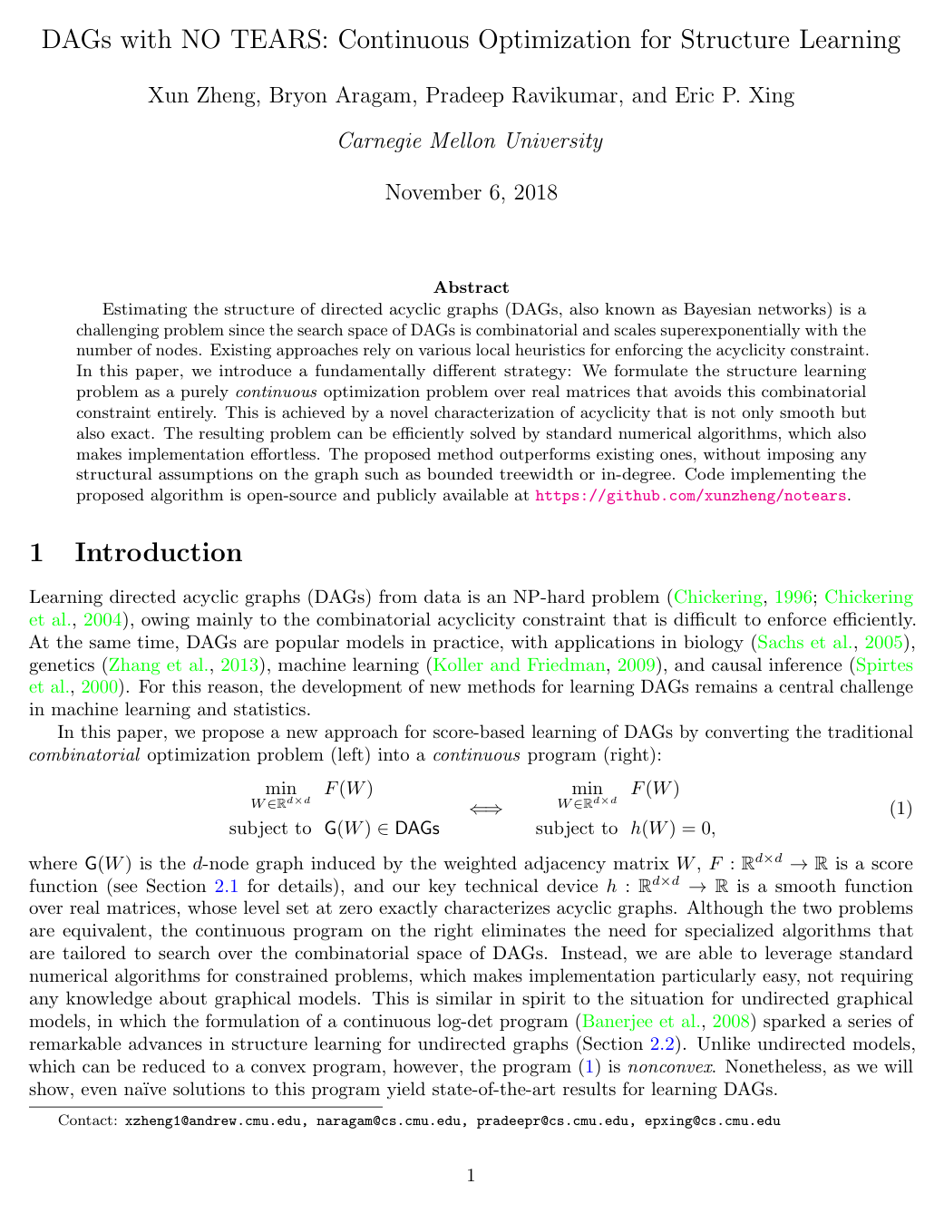
DAGs with NO TEARS: Continuous Optimization for Structure Learning

Xun ZhengBryon AragamPradeep RavikumarEric P. Xing

article2018NeurIPS1,516 citations

Presents a smooth, exact characterization of acyclicity that reformulates directed acyclic graph structure learning as a continuous optimization problem solvable by standard numerical solvers without combinatorial heuristics.

Listen

Learning directed acyclic graphs (DAGs), commonly referred to as Bayesian networks, is essential for causal discovery and understanding complex systems across biology, genetics, and machine learning. Historically, discovering these networks directly from data has been an intractable computational bottleneck. The fundamental challenge stems from the requirement that the learned graph must contain no directed cycles. Because the search space of possible acyclic structures grows superexponentially with the number of variables, existing methods have relied on combinatorial heuristics, local edge-by-edge searches, or restrictive topological assumptions that often fail in real-world, highly interconnected networks.

The article introduces and evaluates a novel mathematical formulation that transforms this traditionally discrete graph search into a smooth, continuous numerical optimization problem. By establishing an exact, differentiable equality constraint based on the matrix exponential to enforce acyclicity, the article develops an algorithm named NOTEARS (Non-combinatorial Optimization via Trace Exponential and Augmented lagRangian for Structure learning). This enables standard, off-the-shelf continuous solvers to simultaneously learn the graph structure and its parameters without combinatorial heuristics.

To evaluate this approach, the authors performed extensive synthetic simulations across varying graph types (Erdös-Rényi and scale-free networks), sample sizes (20 and 1,000 observations), network scales (up to 100 variables), and noise distributions (Gaussian, Exponential, and Gumbel). The method was benchmarked against leading state-of-the-art algorithms, primarily Fast Greedy Search (FGS), as well as exact global optimization baselines and a real-world biological dataset of human immune cell signaling pathways.

The experimental findings show that the proposed continuous framework significantly outperforms traditional greedy methods in structure recovery, particularly as network density and variable counts increase. While greedy algorithms deteriorate rapidly on scale-free graphs containing hub nodes, NOTEARS maintains high true positive rates and lower structural errors across diverse noise distributions. Additionally, incorporating sparsity regularization enables the algorithm to reliably reconstruct networks even in severely data-constrained regimes (such as 20 samples across 100 variables). Evaluations against exact combinatorial solvers confirm that the stationary points obtained by the continuous algorithm are practically equivalent to global optima, and benchmark performance on real-world cellular data matches established biological consensus.

These findings have strong strategic implications for organizations utilizing data-driven causal modeling. By reframing structural learning into standard continuous optimization, implementation is simplified to approximately 50 lines of code, significantly lowering software maintenance costs, reducing algorithmic complexity, and removing the need for domain-specific heuristic tuning. Furthermore, because the algorithm updates all graph parameters globally and simultaneously, it mitigates the risk of missing complex causal dependencies in interconnected systems with hub nodes.

Decision-makers and engineering teams should consider adopting this continuous optimization framework to modernize causal discovery pipelines, replacing fragile combinatorial toolkits with standard numerical optimization solvers. Organizations should implement sparsity penalties when working with limited sample sizes to minimize false discoveries. Next steps should focus on extending the framework to handle non-smooth score functions and developing automated, data-driven thresholds for edge pruning across diverse signal-to-noise environments.

While the algorithm demonstrates robust performance, users should note key boundary conditions. The underlying equality-constrained optimization problem is nonconvex, meaning standard solvers provide local stationary guarantees rather than theoretical global optimality. Furthermore, because calculating the matrix exponential has a cubic computational complexity relative to the number of nodes, users should exercise caution when scaling to extremely large networks without second-order acceleration or sparsity optimizations.

Cover for DAGs with NO TEARS: Continuous Optimization for Structure Learning

Abstract

Estimating the structure of directed acyclic graphs (DAGs, also known as Bayesian networks) is a challenging problem since the search space of DAGs is combinatorial and scales superexponentially with the number of nodes. Existing approaches rely on various local heuristics for enforcing the acyclicity constraint. In this paper, we introduce a fundamentally different strategy: We formulate the structure learning problem as a purely \emph{continuous} optimization problem over real matrices that avoids this combinatorial constraint entirely. This is achieved by a novel characterization of acyclicity that is not only smooth but also exact. The resulting problem can be efficiently solved by standard numerical algorithms, which also makes implementation effortless. The proposed method outperforms existing ones, without imposing any structural assumptions on the graph such as bounded treewidth or in-degree. Code implementing the proposed algorithm is open-source and publicly available at this https URL.

Table of Contents

  • 1 Introduction
  • 2 Background
  • 2.1 Score functions and SEM
  • 2.2 Previous work
  • 2.3 Comparison
  • 3 A new characterization of acyclicity
  • 3.1 Special case: Binary adjacency matrices
  • 3.2 The general case: Weighted adjacency matrices
  • 4 Optimization
  • 4.1 Solving the ECP with augmented Lagrangian
  • 4.2 Solving the unconstrained subproblem
  • 4.3 Thresholding
  • 5 Experiments
  • 5.1 Parameter estimation
  • 5.2 Structure learning
  • 5.3 Comparison to exact global minimizer
  • 5.4 Real-data
  • 6 Discussion
  • References
  • A Details of Proximal Quasi-Newton
  • B Sensitivity of threshold
  • C Sensitivity of weight scale
  • D Experiments
  • D.1 Experiment details
  • D.2 Metrics
  • D.3 Further evaluations

Knowls

  1. Knowl 1 — Smooth Characterization of Acyclicity via Matrix Exponential

    theoretical result

    A matrix W∈Rd×dW \in \mathbb{R}^{d \times d} is the weighted adjacency matrix of a directed acyclic graph (DAG) if and only if:

    h(W)=tr⁡(eW∘W)−d=0h(W) = \operatorname{tr}\left(e^{W \circ W}\right) - d = 0

    where ∘\circ denotes the Hadamard (elementwise) product [W∘W]ij=Wij2[W \circ W]_{ij} = W_{ij}^2, tr⁡(⋅)\operatorname{tr}(\cdot) denotes matrix trace, and eA=∑k=0∞Akk!e^A = \sum_{k=0}^\infty \frac{A^k}{k!} is the matrix exponential.

    The function h:Rd×d→Rh: \mathbb{R}^{d \times d} \to \mathbb{R} is continuously differentiable and non-negative (h(W)≥0h(W) \ge 0 for all W∈Rd×dW \in \mathbb{R}^{d \times d}), with its zero level set corresponding exactly to the space of DAGs. Its matrix gradient is given by:

    ∇h(W)=(eW∘W)T∘2W\nabla h(W) = \left(e^{W \circ W}\right)^T \circ 2W

    Because tr⁡((W∘W)k)\operatorname{tr}((W \circ W)^k) counts all weighted closed walks of length kk (where each edge i→ji \to j contributes weight Wij2W_{ij}^2), h(W)h(W) quantifies graph cyclicity smoothly.

  2. Knowl 2 — Continuous Equality-Constrained Formulation of DAG Structure Learning

    model/method

    Given a data matrix X∈Rn×dX \in \mathbb{R}^{n \times d} of nn observations on dd variables, the combinatorial score-based DAG structure learning problem:

    min⁡W∈Rd×dℓ(W;X)+λ∥W∥1subject to G(W)∈DAGs\min_{W \in \mathbb{R}^{d \times d}} \ell(W; X) + \lambda \|W\|_1 \quad \text{subject to } G(W) \in \text{DAGs}

    is formulated as an equivalent continuous equality-constrained optimization problem:

    min⁡W∈Rd×dℓ(W;X)+λ∥W∥1subject to h(W)=0\min_{W \in \mathbb{R}^{d \times d}} \ell(W; X) + \lambda \|W\|_1 \quad \text{subject to } h(W) = 0

    where ℓ(W;X)=12n∥X−XW∥F2\ell(W; X) = \frac{1}{2n}\|X - XW\|_F^2 is the least-squares loss, ∥W∥1=∑i,j=1d∣Wij∣\|W\|_1 = \sum_{i,j=1}^d |W_{ij}| is an elementwise ℓ1\ell_1-regularization penalty with parameter λ≥0\lambda \ge 0 to encourage sparsity, and h(W)=tr⁡(eW∘W)−dh(W) = \operatorname{tr}(e^{W \circ W}) - d is the smooth acyclicity constraint function.

  3. Knowl 3 — NOTEARS Augmented Lagrangian Optimization Algorithm

    algorithm

    The NOTEARS (Non-combinatorial Optimization via Trace Exponential and Augmented lagRangian for Structure learning) algorithm solves the equality-constrained DAG learning program by solving a sequence of unconstrained augmented Lagrangian subproblems combined with dual gradient ascent and post-hoc thresholding.

    Input: Initial weight matrix W0∈Rd×dW_0 \in \mathbb{R}^{d \times d}, initial Lagrange multiplier α0∈R\alpha_0 \in \mathbb{R}, progress factor c∈(0,1)c \in (0, 1), penalty parameter ρ>0\rho > 0, tolerance ϵ>0\epsilon > 0, threshold ω>0\omega > 0
    Output: Estimated DAG weighted adjacency matrix W^∈Rd×d\widehat{W} \in \mathbb{R}^{d \times d}
    for t=0,1,2,…t = 0, 1, 2, \dots do
        Wt+1←arg⁡min⁡W(ℓ(W;X)+λ∥W∥1+ρ2∣h(W)∣2+αth(W))W_{t+1} \leftarrow \arg\min_W \left( \ell(W; X) + \lambda \|W\|_1 + \frac{\rho}{2}|h(W)|^2 + \alpha_t h(W) \right) with ρ\rho chosen such that h(Wt+1)<c⋅h(Wt)h(W_{t+1}) < c \cdot h(W_t)
        αt+1←αt+ρ⋅h(Wt+1)\alpha_{t+1} \leftarrow \alpha_t + \rho \cdot h(W_{t+1})
        if h(Wt+1)<ϵh(W_{t+1}) < \epsilon then
            W~ECP←Wt+1\widetilde{W}_{\text{ECP}} \leftarrow W_{t+1}
            break
        end if
    end for
    W^←W~ECP∘1(∣W~ECP∣>ω)\widehat{W} \leftarrow \widetilde{W}_{\text{ECP}} \circ \mathbf{1}(|\widetilde{W}_{\text{ECP}}| > \omega)
    return W^\widehat{W}

    Here h(W)=tr⁡(eW∘W)−dh(W) = \operatorname{tr}(e^{W \circ W}) - d, ℓ(W;X)=12n∥X−XW∥F2\ell(W; X) = \frac{1}{2n}\|X - XW\|_F^2, and 1(∣W~ECP∣>ω)\mathbf{1}(|\widetilde{W}_{\text{ECP}}| > \omega) is an elementwise indicator mask setting weights at or below ω\omega to zero.

  4. Knowl 4 — Matrix Exponential Characterization of Acyclicity for Binary Adjacency Matrices

    theoretical result

    A binary adjacency matrix B∈{0,1}d×dB \in \{0, 1\}^{d \times d} defines a directed acyclic graph (DAG) on dd vertices if and only if:

    tr⁡(eB)=d\operatorname{tr}\left(e^B\right) = d

    where eB=∑k=0∞Bkk!e^B = \sum_{k=0}^\infty \frac{B^k}{k!} is the matrix exponential.

    Because (Bk)ii(B^k)_{ii} counts the number of closed walks of length kk starting and ending at node ii, a directed graph is acyclic if and only if tr⁡(Bk)=0\operatorname{tr}(B^k) = 0 for all k≥1k \ge 1. Since all entries of BkB^k are non-negative, ∑k=1∞tr⁡(Bk)k!=tr⁡(eB)−d=0\sum_{k=1}^\infty \frac{\operatorname{tr}(B^k)}{k!} = \operatorname{tr}(e^B) - d = 0 is strictly satisfied if and only if BB contains no directed cycles.

    Under the condition that the spectral radius r(B)<1r(B) < 1, an equivalent characterization is tr⁡(I−B)−1=d\operatorname{tr}(I - B)^{-1} = d, derived from the Neumann series ∑k=0∞Bk=(I−B)−1\sum_{k=0}^\infty B^k = (I - B)^{-1}.

  5. Knowl 5 — Proximal Quasi-Newton Coordinate Descent for L1-Regularized Subproblems

    algorithm

    To solve the unconstrained subproblem min⁡w∈Rpf(w)+λ∥w∥1\min_{w \in \mathbb{R}^p} f(w) + \lambda \|w\|_1 where p=d2p = d^2, w=vec⁡(W)w = \operatorname{vec}(W), and f(w)=ℓ(W;X)+ρ2∣h(W)∣2+αh(W)f(w) = \ell(W; X) + \frac{\rho}{2}|h(W)|^2 + \alpha h(W), proximal quasi-Newton (PQN) minimizes a quadratic approximation using a low-rank L-BFGS Hessian approximation Bk=γkI−QQ^∈Rp×pB_k = \gamma_k I - Q \widehat{Q} \in \mathbb{R}^{p \times p} with memory m≪pm \ll p.

    Input: Initial iterate w0∈Rpw_0 \in \mathbb{R}^p, gradient g0=∇f(w0)g_0 = \nabla f(w_0), active coordinate set S={1,…,p}S = \{1, \dots, p\}, memory size mm, constant c1∈(0,1)c_1 \in (0, 1)
    Output: Optimized parameter vector w∈Rpw \in \mathbb{R}^p
    for k=0,1,2,…k = 0, 1, 2, \dots do
        Shrink SS by removing coordinates jj with wj=0w_j = 0 or small subgradient
        if shrinking stopping criterion is satisfied then
            Reset S←{1,…,p}S \leftarrow \{1, \dots, p\} and reset L-BFGS memory history
        end if
        Compute compact L-BFGS factors Q,R,Q^Q, R, \widehat{Q} and diag⁡(Bk)\operatorname{diag}(B_k) on SS in O(m2∣S∣+m3)O(m^2 |S| + m^3) time
        Compute descent direction dkd_k restricted to SS by coordinate updates d←d+z∗ejd \leftarrow d + z^* e_j in O(m)O(m) time per coordinate:
        a←(Bk)jja \leftarrow (B_k)_{jj}
        b←gj+(Bkd)jb \leftarrow g_j + (B_k d)_j
        c←wj+djc \leftarrow w_j + d_j
        z∗←−c+sign⁡(c−ba)max⁡(∣c−ba∣−λa,0)z^* \leftarrow -c + \operatorname{sign}\left(c - \frac{b}{a}\right) \max\left(\left|c - \frac{b}{a}\right| - \frac{\lambda}{a}, 0\right)
        Perform backtracking line search for step size η∈(0,1]\eta \in (0, 1] satisfying the Armijo condition:
        f(wk+ηdk)≤f(wk)+ηc1(λ∥wk+dk∥1−λ∥wk∥1+gkTdk)f(w_k + \eta d_k) \le f(w_k) + \eta c_1 \left( \lambda \|w_k + d_k\|_1 - \lambda \|w_k\|_1 + g_k^T d_k \right)
        wk+1←wk+ηdkw_{k+1} \leftarrow w_k + \eta d_k
        Update gradient gk+1g_{k+1} and L-BFGS memory restricted to SS
    end for
    return ww
  6. Knowl 6 — Linear Structural Equation Model and Regularized Least-Squares Score

    model/method

    A random vector X=(X1,…,Xd)T∈RdX = (X_1, \dots, X_d)^T \in \mathbb{R}^d is generated according to a linear structural equation model (SEM):

    X=WTX+zX = W^T X + z

    where W=[w1∣⋯∣wd]∈Rd×dW = [w_1 \mid \dots \mid w_d] \in \mathbb{R}^{d \times d} is a weighted adjacency matrix with zero diagonal (Wii=0W_{ii} = 0), Wij≠0W_{ij} \ne 0 indicates a directed edge i→ji \to j, and z=(z1,…,zd)Tz = (z_1, \dots, z_d)^T is a vector of independent, zero-mean noise variables with arbitrary (not necessarily Gaussian) distribution.

    Given an n×dn \times d observational data matrix XX, the graph structure and edge weights are jointly scored via the regularized least-squares objective:

    F(W)=12n∥X−XW∥F2+λ∥W∥1F(W) = \frac{1}{2n} \|X - XW\|_F^2 + \lambda \|W\|_1

    where ∥X−XW∥F2=∑j=1d∥X⋅,j−Xwj∥22\|X - XW\|_F^2 = \sum_{j=1}^d \|X_{\cdot, j} - X w_j\|_2^2 is the sum of squared residuals across all dd linear regressions, and ∥W∥1=∑i,j=1d∣Wij∣\|W\|_1 = \sum_{i,j=1}^d |W_{ij}| is the elementwise ℓ1\ell_1-norm encouraging sparsity.

  7. Knowl 7 — Post-Optimization Hard Thresholding for Graph Rounding

    model/method

    Because numerical optimization of the augmented Lagrangian converges to a stationary point W~ECP\widetilde{W}_{\text{ECP}} satisfying h(W~ECP)≤ϵh(\widetilde{W}_{\text{ECP}}) \le \epsilon for a small numerical tolerance (such as ϵ=10−8\epsilon = 10^{-8}) rather than exact zero, a post-processing elementwise hard-thresholding step is applied:

    W^=W~ECP∘1(∣W~ECP∣>ω)\widehat{W} = \widetilde{W}_{\text{ECP}} \circ \mathbf{1}(|\widetilde{W}_{\text{ECP}}| > \omega)

    where ω>0\omega > 0 is a fixed positive threshold (e.g., ω=0.3\omega = 0.3).

    Because h(W)h(W) quantifies cycle edge weights and non-edge parameters converge close to machine zero, hard thresholding rounds the numerical solution, eliminating small cycle-inducing numerical artifacts and reducing false edge discoveries while preserving true edges.

  8. Knowl 8 — Solution Quality Comparison Between NOTEARS and Exact Integer Programming

    data/table

    The stationary points found by NOTEARS (W^\widehat{W} after thresholding, W~ECP\widetilde{W}_{\text{ECP}} before thresholding) were evaluated against the exact global minimizer WGW_G computed via GOBNILP integer programming on d=10d = 10 nodes across sample sizes n∈{20,1000}n \in \{20, 1000\} and λ∈{0,0.5}\lambda \in \{0, 0.5\} on Erdős–Rényi (ER1, ER2, ER4) and Scale-Free (SF4) graphs:

    nn λ\lambda Graph F(Wtrue)F(W_{\text{true}}) F(WG)F(W_G) F(W^)F(\widehat{W}) F(W~ECP)F(\widetilde{W}_{\text{ECP}}) ∥W^−WG∥F\|\widehat{W} - W_G\|_F ∥Wtrue−WG∥F\|W_{\text{true}} - W_G\|_F
    20 0.00 ER1 5.01 3.69 5.19 3.73 0.09 3.54
    20 0.50 ER1 12.43 9.90 10.69 9.88 0.11 2.76
    1000 0.00 ER1 4.96 4.93 4.97 4.92 0.03 0.35
    1000 0.50 ER1 12.37 10.53 11.01 10.58 0.11 2.47
    20 0.00 ER2 5.11 3.85 5.36 3.88 0.07 3.38
    20 0.50 ER2 16.04 12.81 13.49 12.90 0.12 3.15
    1000 0.00 ER2 4.99 4.97 5.02 4.95 0.02 0.40
    1000 0.50 ER2 15.93 13.32 14.03 13.46 0.12 2.95
    20 0.00 ER4 4.76 3.66 5.23 3.88 0.08 4.25
    20 0.50 ER4 28.24 16.38 19.81 16.82 0.15 6.66
    1000 0.00 ER4 5.03 5.00 5.50 4.97 0.00 0.46
    1000 0.50 ER4 28.51 18.29 29.91 18.69 0.13 5.76
    20 0.00 SF4 4.99 3.77 4.70 3.85 0.08 3.31
    20 0.50 SF4 23.33 16.19 17.31 16.69 0.15 5.08
    1000 0.00 SF4 4.96 4.94 5.05 4.99 0.04 0.29
    1000 0.50 SF4 23.29 17.56 19.70 18.43 0.13 4.34

    The data demonstrates that despite the theoretical nonconvexity of the equality constraint, the local stationary points returned by NOTEARS attain score values F(W^)F(\widehat{W}) closely matching the global optimum F(WG)F(W_G), and parameter deviations ∥W^−WG∥F≤0.15\|\widehat{W} - W_G\|_F \le 0.15 remain consistently low across all graph types and sample sizes.

  9. Knowl 9 — Empirical Structure Recovery Performance Across Graph Topologies and Noise Distributions

    empirical result

    In synthetic benchmarks on random graphs with d∈{10,20,50,100}d \in \{10, 20, 50, 100\} nodes and sample sizes n∈{20,1000}n \in \{20, 1000\}, NOTEARS was compared against Fast Greedy Search (FGS) under Gaussian, Exponential, and Gumbel noise distributions on Erdős–Rényi (ER) and Scale-Free (SF) topologies:

    • On sparse graphs with few edges (ER-2), FGS and NOTEARS perform competitively.
    • On denser graphs (SF-4 and ER-4), NOTEARS substantially outperforms FGS, exhibiting significantly lower Structural Hamming Distance (SHD) and lower False Discovery Rate (FDR), with performance advantages widening as graph size dd increases up to 100.
    • NOTEARS achieves consistently strong structure recovery across non-Gaussian noise models (Exponential and Gumbel) without relying on distributional knowledge.
    • In the small sample regime (n=20n = 20), ℓ1\ell_1-regularization (NOTEARS-L1) is necessary and effective for maintaining low FDR and preventing severe overfitting.
  10. Knowl 10 — Benchmark Evaluation on Sachs Cell Signaling Dataset

    empirical result

    On the real-world flow cytometry dataset from Sachs et al. (2005) measuring expression levels of 11 proteins and phospholipids across n=7466n = 7466 human immune cells (with a consensus biological ground truth graph containing 20 directed edges):

    • NOTEARS estimated a DAG with 16 directed edges and achieved a Structural Hamming Distance (SHD) of 22 relative to the consensus network.
    • Fast Greedy Search (FGS) estimated a graph with 17 directed edges and achieved an identical SHD of 22.
  11. Knowl 11 — Methodological and Computational Limitations of NOTEARS

    limitation

    The NOTEARS approach has four primary limitations:

    1. Nonconvexity: The constraint set {W∈Rd×d:h(W)=0}\{W \in \mathbb{R}^{d \times d} : h(W) = 0\} is nonconvex; continuous solvers are guaranteed to find stationary points rather than global minimizers, leaving open the existence of pathological instances with poor local minima.
    2. Cubic Computational Complexity: Computing the matrix exponential eW∘We^{W \circ W} and its gradient requires O(d3)O(d^3) operations per evaluation, making scaling to very large networks (d≫1000d \gg 1000) computationally demanding without additional structural or numerical approximations.
    3. Score Smoothness Requirement: The formulation relies on continuous gradients of the loss function ℓ(W;X)\ell(W; X), precluding direct optimization of discrete, non-smooth scoring criteria such as BDe or MDL without continuous smoothing approximations.
    4. Fixed Thresholding Parameter: Post-processing hard thresholding relies on a fixed threshold ω>0\omega > 0 (e.g., ω=0.3\omega = 0.3) rather than a data-driven rule that automatically adapts to graph density and signal-to-noise ratio.

Coverage note — No substantial contributed material was omitted; baseline comparisons with PC and LiNGAM (which yielded substantially inferior performance) and sensitivity analyses for edge weights and thresholds are summarized within the relevant methodological, empirical, and limitation knowls.

References

  1. 1.A. H. Al-Mohy and N. J. Higham. A New Scaling and Squaring Algorithm for the Matrix Exponential. SIAM Journal on Matrix Analysis and Applications, 2009.
  2. 2.B. Aragam and Q. Zhou. Concave penalized estimation of sparse Gaussian Bayesian networks. Journal of Machine Learning Research, 16:2273–2328, 2015.
  3. 3.B. Aragam, A. A. Amini, and Q. Zhou. Learning directed acyclic graphs with penalized neighbourhood regression. Submitted, arXiv:1511.08963, 2016.
  4. 4.O. Banerjee, L. El Ghaoui, and A. d’Aspremont. Model selection through sparse maximum likelihood estimation for multivariate Gaussian or binary data. Journal of Machine Learning Research, 9:485–516, 2008.
  5. 5.A.-L. Barab´asi and R. Albert. Emergence of scaling in random networks. Science, 286(5439):509–512, 1999.
  6. 6.A. Botev, H. Ritter, and D. Barber. Practical gauss-newton optimisation for deep learning. arXiv preprint arXiv:1706.03662, 2017.
  7. 7.L. Bottou, F. E. Curtis, and J. Nocedal. Optimization methods for large-scale machine learning. arXiv preprint arXiv:1606.04838, 2016.
  8. 8.R. R. Bouckaert. Probabilistic network construction using the minimum description length principle. In European conference on symbolic and quantitative approaches to reasoning and uncertainty, pages 41–48. Springer, 1993.
  9. 9.O. Bousquet and L. Bottou. The tradeoffs of large scale learning. In Advances in neural information processing systems, pages 161–168, 2008.
  10. 10.R. H. Byrd, P. Lu, J. Nocedal, and C. Zhu. A limited memory algorithm for bound constrained optimization. SIAM Journal on Scientific Computing, 1995.
  11. 11.E. Y.-J. Chen, Y. Shen, A. Choi, and A. Darwiche. Learning bayesian networks with ancestral constraints. In Advances in Neural Information Processing Systems, pages 2325–2333, 2016.
  12. 12.D. M. Chickering. Learning Bayesian networks is NP-complete. In Learning from data, pages 121–130. Springer, 1996.
  13. 13.D. M. Chickering. Optimal structure identification with greedy search. Journal of Machine Learning Research, 3:507–554, 2003.
  14. 14.D. M. Chickering and D. Heckerman. Efficient approximations for the marginal likelihood of Bayesian networks with hidden variables. Machine Learning, 29(2-3):181–212, 1997.
  15. 15.D. M. Chickering, D. Heckerman, and C. Meek. Large-sample learning of Bayesian networks is NP-hard. Journal of Machine Learning Research, 5:1287–1330, 2004.
  16. 16.J. Cussens. Bayesian network learning with cutting planes. arXiv preprint arXiv:1202.3713, 2012.
  17. 17.J. Cussens, D. Haws, and M. Studen`y. Polyhedral aspects of score equivalence in bayesian network structure learning. Mathematical Programming, 164(1-2):285–324, 2017.
  18. 18.B. Ellis and W. H. Wong. Learning causal Bayesian network structures from experimental data. Journal of the American Statistical Association, 103(482), 2008.
  19. 19.J. Friedman, T. Hastie, and R. Tibshirani. Sparse inverse covariance estimation with the Graphical Lasso. Biostatistics, 9(3):432–441, 2008.
  20. 20.F. Fu and Q. Zhou. Learning sparse causal Gaussian networks with experimental intervention: Regularization and coordinate descent. Journal of the American Statistical Association, 108(501):288–300, 2013.
  21. 21.J. A. G´amez, J. L. Mateo, and J. M. Puerta. Learning Bayesian networks by hill climbing: Efficient methods based on progressive restriction of the neighborhood. Data Mining and Knowledge Discovery, 22(1-2): 106–148, 2011.
  22. 22.M. Grant and S. Boyd. CVX: Matlab software for disciplined convex programming, version 2.1. http: //cvxr.com/cvx, Mar. 2014.
  23. 23.J. Gu, F. Fu, and Q. Zhou. Penalized estimation of directed acyclic graphs from discrete data. Statistics and Computing, DOI: 10.1007/s11222-018-9801-y, 2018.
  24. 24.F. Harary and B. Manvel. On the number of cycles in a graph. Matematick`y ˇcasopis, 1971.
  25. 25.D. Heckerman, D. Geiger, and D. M. Chickering. Learning Bayesian networks: The combination of knowledge and statistical data. Machine learning, 20(3):197–243, 1995.
  26. 26.C.-J. Hsieh, M. A. Sustik, I. S. Dhillon, and P. Ravikumar. Quic: quadratic approximation for sparse inverse covariance estimation. Journal of Machine Learning Research, 15(1):2911–2947, 2014.
  27. 27.D. P. Kingma and J. Ba. Adam: A method for stochastic optimization. arXiv preprint arXiv:1412.6980, 2014.
  28. 28.D. Koller and N. Friedman. Probabilistic graphical models: principles and techniques. MIT press, 2009.
  29. 29.J. Kuipers, G. Moffa, and D. Heckerman. Addendum on the scoring of gaussian directed acyclic graphical models. The Annals of Statistics, pages 1689–1691, 2014.
  30. 30.P.-L. Loh and P. B¨uhlmann. High-dimensional learning of linear causal networks via inverse covariance estimation. Journal of Machine Learning Research, 15:3065–3105, 2014.
  31. 31.A. Nemirovski. Optimization II: Standard Numerical Methods for Nonlinear Continuous Optimization. 1999.
  32. 32.Y. Nesterov. Smooth minimization of non-smooth functions. Mathematical Programming, 2005.
  33. 33.T. Niinim¨aki, P. Parviainen, and M. Koivisto. Structure discovery in bayesian networks by sampling partial orders. Journal of Machine Learning Research, 17(1):2002–2048, 2016.
  34. 34.J. Nocedal and S. J. Wright. Numerical Optimization. 2006.
  35. 35.S. Ott and S. Miyano. Finding optimal gene networks using biological constraints. Genome Informatics, 14: 124–133, 2003.
  36. 36.J. Ramsey, M. Glymour, R. Sanchez-Romero, and C. Glymour. A million variables and more: the fast greedy equivalence search algorithm for learning high-dimensional graphical causal models, with an application to functional magnetic resonance images. International Journal of Data Science and Analytics, pages 1–9, 2016.
  37. 37.R. W. Robinson. Counting unlabeled acyclic digraphs. In Combinatorial mathematics V, pages 28–43. Springer, 1977.
  38. 38.K. Sachs, O. Perez, D. Pe’er, D. A. Lauffenburger, and G. P. Nolan. Causal protein-signaling networks derived from multiparameter single-cell data. Science, 308(5721):523–529, 2005.
  39. 39.M. Scanagatta, C. P. de Campos, G. Corani, and M. Zaffalon. Learning bayesian networks with thousands of variables. In Advances in Neural Information Processing Systems, pages 1864–1872, 2015.
  40. 40.M. Scanagatta, G. Corani, C. P. de Campos, and M. Zaffalon. Learning treewidth-bounded bayesian networks with thousands of variables. In Advances in Neural Information Processing Systems, pages 1462–1470, 2016.
  41. 41.M. Schmidt, A. Niculescu-Mizil, and K. Murphy. Learning graphical model structure using L1-regularization paths. In AAAI, volume 7, pages 1278–1283, 2007.
  42. 42.M. Schmidt, E. Berg, M. Friedlander, and K. Murphy. Optimizing costly functions with simple constraints: A limited-memory projected quasi-newton algorithm. In Artificial Intelligence and Statistics, pages 456–463, 2009.
  43. 43.S. Shimizu, P. O. Hoyer, A. Hyv¨arinen, and A. Kerminen. A linear non-Gaussian acyclic model for causal discovery. Journal of Machine Learning Research, 7:2003–2030, 2006.
  44. 44.T. Silander and P. Myllymaki. A simple approach for finding the globally optimal bayesian network structure. In Proceedings of the 22nd Conference on Uncertainty in Artificial Intelligence, 2006.
  45. 45.A. P. Singh and A. W. Moore. Finding optimal bayesian networks by dynamic programming. 2005.
  46. 46.P. Spirtes and C. Glymour. An algorithm for fast recovery of sparse causal graphs. Social Science Computer Review, 9(1):62–72, 1991.
  47. 47.P. Spirtes, C. Glymour, and R. Scheines. Causation, prediction, and search, volume 81. The MIT Press, 2000.
  48. 48.G. Taylor, R. Burmeister, Z. Xu, B. Singh, A. Patel, and T. Goldstein. Training neural networks without gradients: A scalable admm approach. In International Conference on Machine Learning, pages 2722–2731, 2016.
  49. 49.M. Teyssier and D. Koller. Ordering-based search: A simple and effective algorithm for learning bayesian networks. In Uncertainty in Artifical Intelligence (UAI), 2005.
  50. 50.I. Tsamardinos, L. E. Brown, and C. F. Aliferis. The max-min hill-climbing Bayesian network structure learning algorithm. Machine Learning, 65(1):31–78, 2006.
  51. 51.P. Van Beek and H.-F. Hoffmann. Machine learning of bayesian networks using constraint programming. In International Conference on Principles and Practice of Constraint Programming, pages 429–445. Springer, 2015.
  52. 52.S. van de Geer and P. B¨uhlmann. `0-penalized maximum likelihood for sparse directed acyclic graphs. Annals of Statistics, 41(2):536–567, 2013.
  53. 53.X. Wang, D. Dunson, and C. Leng. No penalty no tears: Least squares in high-dimensional linear models. In International Conference on Machine Learning, pages 1814–1822, 2016.
  54. 54.D. J. Watts and S. H. Strogatz. Collective dynamics of small-world networks. nature, 393(6684):440, 1998.
  55. 55.J. Xiang and S. Kim. A* Lasso for learning a sparse Bayesian network structure for continuous variables. In Advances in Neural Information Processing Systems, pages 2418–2426, 2013.
  56. 56.M. Yuan and Y. Lin. Model selection and estimation in the Gaussian graphical model. Biometrika, 94(1): 19–35, 2007.
  57. 57.B. Zhang, C. Gaiteri, L.-G. Bodea, Z. Wang, J. McElwee, A. A. Podtelezhnikov, C. Zhang, T. Xie, L. Tran, R. Dobrin, et al. Integrated systems approach identifies genetic nodes and networks in late-onset alzheimer’s disease. Cell, 153(3):707–720, 2013.
  58. 58.K. Zhong, I. E.-H. Yen, I. S. Dhillon, and P. K. Ravikumar. Proximal quasi-newton for computationally intensive l1-regularized m-estimators. In Advances in Neural Information Processing Systems, pages 2375–2383, 2014.
  59. 59.Q. Zhou. Multi-domain sampling with applications to structural inference of Bayesian networks. Journal of the American Statistical Association, 106(496):1317–1330, 2011.
  60. 60.S. Zhou. Thresholding procedures for high dimensional variable selection and statistical estimation. In Advances in Neural Information Processing Systems, pages 2304–2312, 2009.

Citation

MLA
Zheng, X., et al. “DAGs with NO TEARS: Continuous Optimization for Structure Learning”. arXiv, 2018, http://arxiv.org/abs/1803.01422v2.
APA
Zheng, X., Aragam, B., Ravikumar, P., & Xing, E. P. (2018). DAGs with NO TEARS: Continuous Optimization for Structure Learning. arXiv. http://arxiv.org/abs/1803.01422v2
Chicago
Zheng, X., B. Aragam, P. Ravikumar, and E. P. Xing. 2018. “DAGs with NO TEARS: Continuous Optimization for Structure Learning”. arXiv. http://arxiv.org/abs/1803.01422v2.
Harvard
Zheng, X. et al. (2018) “DAGs with NO TEARS: Continuous Optimization for Structure Learning”, arXiv [Preprint]. Available at: http://arxiv.org/abs/1803.01422v2.
Vancouver
1. Zheng X, Aragam B, Ravikumar P, Xing EP (2018) DAGs with NO TEARS: Continuous Optimization for Structure Learning. arXiv

BibTeX

@article{zheng2018dags,
  title = {DAGs with NO TEARS: Continuous Optimization for Structure Learning},
  author = {Zheng, Xun and Aragam, Bryon and Ravikumar, Pradeep and Xing, Eric P.},
  year = {2018},
  journal = {arXiv},
  url = {http://arxiv.org/abs/1803.01422v2},
  eprint = {1803.01422}
}
Metadata:arXiv

Source Code

This paper has an official code repository available. Click below to access the source code.

View Repository

Access the Paper

This paper is available from its original source. Click below to access the PDF.

Open PDF
License: Authors