Pathfinder: Parallel quasi-Newton variational inference

Lu ZhangBob CarpenterAndrew GelmanAki Vehtari

article2022JMLR64 citations

Introduces Pathfinder, a parallel variational inference algorithm that constructs normal approximations along quasi-Newton optimization trajectories to produce high-quality posterior draws with one to two orders of magnitude fewer gradient evaluations than standard methods.

Listen

Bayesian statistical computation is widely used across scientific and industrial applications, but modern complex models often require substantial computational time and resources. Standard Markov chain Monte Carlo (MCMC) sampling methods provide asymptotically exact solutions but are computationally intensive and frequently suffer from slow initial warmup phases or become trapped in local minor modes. Faster approximate methods, such as automatic differentiation variational inference (ADVI), often struggle to converge due to the high variance of stochastic gradient estimates and inherently sequential optimization loops.

The article introduces Pathfinder, a fast variational inference algorithm designed to sample approximately from differentiable probability distributions. Its primary objective is to evaluate whether constructing local normal approximations along quasi-Newton optimization trajectories can produce accurate, robust posterior approximations and rapid initializations for MCMC while drastically reducing computation time.

The authors evaluated the algorithm on a benchmark suite of 20 diverse Bayesian models spanning generalized linear models, Gaussian processes, differential equations, and time series, supplemented by high-dimensional case studies. Pathfinder uses a quasi-Newton optimization trajectory (specifically L-BFGS) to move from random initial points toward high-probability regions. Along this path, it constructs local normal approximations using inverse Hessian estimates for local curvature, evaluates the evidence lower bound in parallel to pick the optimal approximation, and draws samples. A multi-path extension runs several trajectories in parallel and applies Pareto-smoothed importance resampling to handle non-normal distributions and filter out inferior local modes.

Key findings show that Pathfinder produces approximate draws that range from slightly worse to significantly better than mean-field and dense ADVI, and comparable to short chains of Hamiltonian Monte Carlo, as measured by 1-Wasserstein distance. Computationally, Pathfinder achieved these results requiring one to two orders of magnitude fewer probability density and gradient evaluations—evaluating approximately 30 to 50 times fewer operations than baseline methods on average. In an applied Gaussian process case study, initializing MCMC chains with Pathfinder successfully avoided minor modes and cut single-chain warmup runtimes by roughly two-thirds.

These results demonstrate that incorporating curvature information via quasi-Newton methods dramatically accelerates approximate Bayesian computation and enhances workflow reliability. Using Pathfinder as a standalone variational approximation or as a drop-in replacement for the initial phase of MCMC warmup reduces computing costs, lowers developer wait times, and diminishes the risk of chains stalling in minor modes.

The authors recommend adopting multi-path Pathfinder with Pareto-smoothed importance resampling as standard practice for fast exploratory analysis and MCMC initialization. Future extensions could incorporate stochastic gradient subsampling to handle massive datasets and integrate Bayesian optimization to fine-tune point selection along optimization paths.

The article notes that confidence should be tempered in high-dimensional distributions with severe multimodality, highly non-normal geometries, or weak parameter identifiability, where approximations can become overly concentrated. For such complex models, the authors advise using Pathfinder primarily as an initialization tool followed by full stochastic MCMC sampling.

arXiv: 2108.03782
Cover for Pathfinder: Parallel quasi-Newton variational inference

Abstract

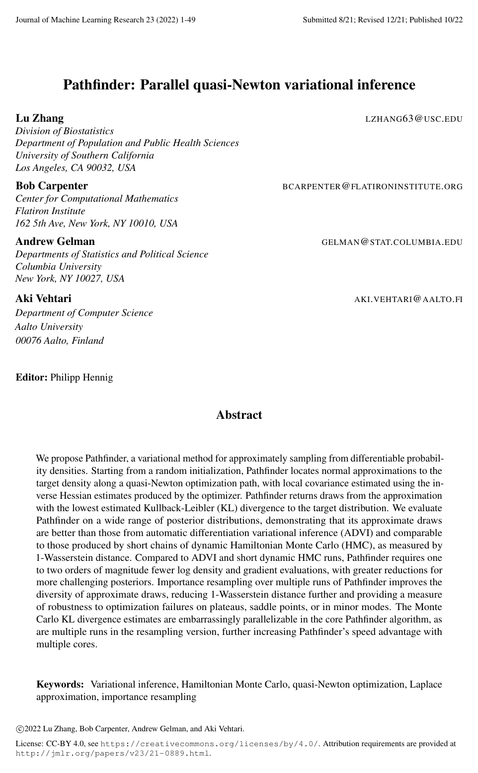
We propose Pathfinder, a variational method for approximately sampling from differentiable probability densities. Starting from a random initialization, Pathfinder locates normal approximations to the target density along a quasi-Newton optimization path, with local covariance estimated using the inverse Hessian estimates produced by the optimizer. Pathfinder returns draws from the approximation with the lowest estimated Kullback-Leibler (KL) divergence to the target distribution. We evaluate Pathfinder on a wide range of posterior distributions, demonstrating that its approximate draws are better than those from automatic differentiation variational inference (ADVI) and comparable to those produced by short chains of dynamic Hamiltonian Monte Carlo (HMC), as measured by 1-Wasserstein distance. Compared to ADVI and short dynamic HMC runs, Pathfinder requires one to two orders of magnitude fewer log density and gradient evaluations, with greater reductions for more challenging posteriors. Importance resampling over multiple runs of Pathfinder improves the diversity of approximate draws, reducing 1-Wasserstein distance further and providing a measure of robustness to optimization failures on plateaus, saddle points, or in minor modes. The Monte Carlo KL divergence estimates are embarrassingly parallelizable in the core Pathfinder algorithm, as are multiple runs in the resampling version, further increasing Pathfinder’s speed advantage with multiple cores.

Table of Contents

  • 1. Introduction
  • 2. Pathfinder
  • 2.1 Pathfinder algorithm
  • 2.2 Multi-path Pathfinder algorithm
  • 2.3 L-BFGS optimization
  • 2.4 Local density approximations along the optimization path
  • 2.5 Sampling from the approximation and evaluating the log density of a draw
  • 2.6 Estimating KL divergence from the approximate densities
  • 2.7 Pareto-smoothed importance resampling
  • 2.8 Related methods
  • 3. Experiments
  • 3.1 Evaluating Pathfinder as variational inference
  • 3.2 Sensitivity to tuning parameters
  • 3.3 Pathfinder for posteriors with challenging geometry
  • 4. Using Pathfinder to initialize MCMC
  • 5. Discussion
  • Acknowledgments
  • Appendix A. Derivation of (4)
  • Appendix B. 1-Wasserstein distance
  • Appendix C. Importance sampling
  • Appendix D. ELBO comparison for simulation studies in Section 3.1
  • Appendix E. Laplace approximation for simulation studies in Section 3.1
  • References

Knowls

  1. Knowl 1 — Pathfinder’s quasi-Newton variational approximation

    model/method

    Pathfinder approximates a differentiable target density p(θ)p(\theta) known up to a normalizing constant, with parameter vector θ∈RN\theta\in\mathbb{R}^N. It draws an initial point θ(0)\theta^{(0)} from an initialization distribution π0\pi_0, then runs L-BFGS on the log density ℓ(θ)=log⁡p(θ)\ell(\theta)=\log p(\theta) to produce an optimization path θ(0),…,θ(L)\theta^{(0)},\ldots,\theta^{(L)}.

    At each path point θ(l)\theta^{(l)}, Pathfinder uses the inverse-Hessian approximation produced from the L-BFGS trajectory to define a multivariate normal approximation

    ql(θ)=Normal⁡ ⁣(θ∣μ(l),Σ(l)),μ(l)=θ(l)+Σ(l)∇ℓ(θ(l)).q_l(\theta)=\operatorname{Normal}\!\left(\theta\mid \mu^{(l)},\Sigma^{(l)}\right), \qquad \mu^{(l)}=\theta^{(l)}+\Sigma^{(l)}\nabla\ell(\theta^{(l)}).

    The algorithm draws KK samples from every qlq_l, evaluates their target and approximation log densities, and estimates each approximation’s evidence lower bound (ELBO). It selects the path index with the largest estimated ELBO and returns MM samples from that selected normal approximation together with their approximation log densities.

    The optimization path can move from the tail through the high-probability region toward a mode or, for an unbounded density, toward a pole. Evaluating all candidate approximations after the L-BFGS run is embarrassingly parallel over path points and samples; L-BFGS is therefore the principal serial component. The default experimental settings were Lmax⁡=1000L_{\max}=1000, relative convergence tolerance 10−1310^{-13}, L-BFGS history size J=6J=6, and K=5K=5 Monte Carlo samples for ELBO estimation.

  2. Knowl 2 — Multi-path Pathfinder with Pareto-smoothed importance resampling

    algorithm

    Multi-path Pathfinder runs II independent single-path Pathfinder instances in parallel. Run ii returns MM samples ϕ(i,1),…,ϕ(i,M)\phi^{(i,1)},\ldots,\phi^{(i,M)} from its ELBO-selected normal approximation qiq_i. The resulting proposal is treated as an equally weighted mixture with an augmented component index ii:

    q~(ϕ,i)=1Iqi(ϕ),p~(ϕ,i)=1Ip(ϕ).\widetilde q(\phi,i)=\frac{1}{I}q_i(\phi), \qquad \widetilde p(\phi,i)=\frac{1}{I}p(\phi).

    For every candidate sample, the algorithm computes the importance ratio using the target log density and the corresponding component proposal log density. It applies Pareto-smoothed importance sampling to the ratios and resamples RR samples with replacement, with probabilities proportional to the smoothed weights. The output is a set of draws rather than weighted samples, which makes the result convenient for estimating expectations and quantiles or initializing MCMC.

    The mixture allows different optimization paths to represent different regions and non-normal structure. Importance resampling tends to downweight paths trapped in minor modes, saddle points, or plateaus, and reduces variability caused by random initialization and noisy ELBO estimates. The II Pathfinder runs are independent and parallelizable; the resampling step waits for all runs but is computationally small. In the experiments, I=20I=20, M=100M=100, and R=100R=100 were used.

  3. Knowl 3 — Linear-in-dimension sampling from the L-BFGS covariance

    model/method

    Pathfinder represents each local covariance as a diagonal-plus-low-rank L-BFGS inverse-Hessian approximation rather than forming or factorizing a dense N×NN\times N matrix. For a history of JJ accepted position and gradient updates, let S,Z∈RN×JS,Z\in\mathbb{R}^{N\times J} contain those updates, let D=diag⁡(α)D=\operatorname{diag}(\alpha) be a positive diagonal matrix, and let E∈RJ×JE\in\mathbb{R}^{J\times J} satisfy Eij=SiTZjE_{ij}=S_i^\mathsf{T}Z_j for i≤ji\leq j and Eij=0E_{ij}=0 otherwise. Define ηi=SiTZi\eta_i=S_i^\mathsf{T}Z_i and

    β=[DZ    S],γ=[0−E−1−E−TE−T(diag⁡(η)+ZTDZ)E−1].\beta=[DZ\;\;S], \qquad \gamma= \begin{bmatrix} 0 & -E^{-1}\\ -E^{-\mathsf{T}} & E^{-\mathsf{T}}\left(\operatorname{diag}(\eta)+Z^\mathsf{T}DZ\right)E^{-1} \end{bmatrix}.

    The covariance is

    Σ=D+βγβT.\Sigma=D+\beta\gamma\beta^\mathsf{T}.

    Let QR~=D−1/2βQ\widetilde R=D^{-1/2}\beta be a thin QR factorization, where Q∈RN×2JQ\in\mathbb{R}^{N\times 2J} has orthonormal columns, and let PP complete QQ to an orthogonal basis. Define the small Cholesky factor L~\widetilde L by

    L~L~T=I2J+R~γR~T.\widetilde L\widetilde L^\mathsf{T}=I_{2J}+\widetilde R\gamma\widetilde R^\mathsf{T}.

    Then Σ=TTT\Sigma=TT^\mathsf{T} for T=D1/2[QL~    P]T=D^{1/2}[Q\widetilde L\;\;P]. If u∼Normal⁡(0,IN)u\sim\operatorname{Normal}(0,I_N), a draw from Normal⁡(μ,Σ)\operatorname{Normal}(\mu,\Sigma) can be generated as

    ϕ=μ+D1/2{Q(L~−I2J)QTu+u}.\phi=\mu+D^{1/2}\left\{Q(\widetilde L-I_{2J})Q^\mathsf{T}u+u\right\}.

    The approximation log density is evaluated without solving an N×NN\times N system:

    log⁡q(ϕ)=−12(log⁡∣Σ∣+uTu+Nlog⁡(2π)),log⁡∣Σ∣=log⁡∣D∣+2log⁡∣L~∣.\log q(\phi)=-\frac{1}{2}\left(\log|\Sigma|+u^\mathsf{T}u+N\log(2\pi)\right), \qquad \log|\Sigma|=\log|D|+2\log|\widetilde L|.

    Sampling and log-density evaluation require O(NJ2+J3)O(NJ^2+J^3) operations and O(NJ+J2)O(NJ+J^2) memory, rather than the O(N3)O(N^3) operations and O(N2)O(N^2) memory associated with dense factorization. With fixed small JJ, the cost is linear in the parameter dimension NN.

  4. Knowl 4 — ELBO-based selection along the optimization path

    equation

    For a candidate normal approximation ql(θ)=Normal⁡(θ∣μ(l),Σ(l))q_l(\theta)=\operatorname{Normal}(\theta\mid\mu^{(l)},\Sigma^{(l)}) and target density p(θ∣y)p(\theta\mid y), Pathfinder selects the approximation minimizing the forward variational divergence KL⁡(ql ∥ p)\operatorname{KL}(q_l\,\|\,p), equivalently maximizing the ELBO. If ϕ(1),…,ϕ(K)\phi^{(1)},\ldots,\phi^{(K)} are independent draws from qlq_l, the Monte Carlo selection criterion is

    L^l=1K∑k=1K[log⁡p ⁣(ϕ(k))−log⁡ql ⁣(ϕ(k))].\widehat{\mathcal L}_l = \frac{1}{K}\sum_{k=1}^{K} \left[\log p\!\left(\phi^{(k)}\right)-\log q_l\!\left(\phi^{(k)}\right)\right].

    Here KK is the number of Monte Carlo draws, log⁡p\log p may be an unnormalized target log density, and the omitted normalizing constant is common to all path points. Thus the selected index is l∗=arg⁡max⁡lL^ll^*=\arg\max_l\widehat{\mathcal L}_l. The KK samples and target-density evaluations for different path points can be generated and evaluated independently, so ELBO estimation is parallelizable. The paper used K=5K=5 by default and used a Pareto-kk diagnostic to assess instability of the importance-weight-related Monte Carlo calculations.

  5. Knowl 5 — Adaptive diagonal inverse-Hessian recovery

    algorithm

    Pathfinder reconstructs a diagonal base inverse-Hessian estimate from the L-BFGS trajectory rather than reusing the optimizer’s scaled-identity diagonal. For consecutive path points, define the position and gradient updates

    s(l)=θ(l)−θ(l−1),z(l)=∇ℓ(θ(l−1))−∇ℓ(θ(l)).s^{(l)}=\theta^{(l)}-\theta^{(l-1)}, \qquad z^{(l)}=\nabla\ell(\theta^{(l-1)})-\nabla\ell(\theta^{(l)}).

    Starting from α(0)=1N\alpha^{(0)}=\mathbf{1}_N, the recovery procedure scans the path, applies a numerical curvature filter with threshold ϵ=10−12\epsilon=10^{-12} to reject unstable update pairs, and retains an indicator ξ(l)\xi^{(l)} for every accepted pair. For an accepted update, define

    a=z(l)Tdiag⁡(α(l−1))z(l),b=z(l)Ts(l),c=s(l)Tdiag⁡(α(l−1))−1s(l).a=z^{(l)\mathsf{T}}\operatorname{diag}(\alpha^{(l-1)})z^{(l)}, \qquad b=z^{(l)\mathsf{T}}s^{(l)}, \qquad c=s^{(l)\mathsf{T}}\operatorname{diag}(\alpha^{(l-1)})^{-1}s^{(l)}.

    Each diagonal element is updated as

    αn(l)=[abαn(l−1)+(zn(l))2b−a(sn(l))2bc(αn(l−1))2]−1,n=1,…,N.\alpha_n^{(l)}= \left[ \frac{a}{b\alpha_n^{(l-1)}} +\frac{(z_n^{(l)})^2}{b} -\frac{a(s_n^{(l)})^2}{bc(\alpha_n^{(l-1)})^2} \right]^{-1}, \qquad n=1,\ldots,N.

    If the pair is rejected, α(l)=α(l−1)\alpha^{(l)}=\alpha^{(l-1)} and ξ(l)=0\xi^{(l)}=0. The stored updates and indicators let Pathfinder reconstruct the low-rank covariance factors for any path point without storing a full inverse-Hessian matrix. The recovery pass costs O(LJN)O(LJN) for path length LL, dimension NN, and history size JJ.

  6. Knowl 6 — Benchmark design across posterior models

    experimental setup

    The main benchmark used 20 Bayesian models and data sets from the posteriordb evaluation collection, including generalized linear, hierarchical, Gaussian-process, mixture, differential-equation, hidden-Markov, and time-series models. Each model had approximately 10,000 roughly independent reference posterior draws. All parameters were transformed to an unconstrained RN\mathbb{R}^N representation with the required Jacobian adjustment, and approximation quality was evaluated on that unconstrained scale.

    For each method and model, the authors performed 100 independent runs and generated 100 approximate draws per run. Single-path Pathfinder used Lmax⁡=1000L_{\max}=1000, relative tolerance 10−1310^{-13}, history size J=6J=6, ELBO sample size K=5K=5, and M=100M=100. Multi-path Pathfinder used I=20I=20 independent paths, M=100M=100 draws per path, and R=100R=100 final resampled draws. The comparison methods were Stan phase-I adaptive HMC using a unit metric, step-size adaptation, maximum tree depth 10, and the last draw from 75 iterations; dense ADVI; and mean-field ADVI. All methods used random initial values from Uniform⁡(−2,2)\operatorname{Uniform}(-2,2).

    Approximation quality was measured by the discrete 1-Wasserstein distance between 100 approximate draws and 100 reference draws. This metric was chosen because it is symmetric and is a proper distance metric, unlike the asymmetric KL divergence used for optimization.

  7. Knowl 7 — Accuracy and computational advantage over ADVI and short HMC

    empirical result

    Across the 20 benchmark posteriors, single-path and multi-path Pathfinder generally had smaller and more stable 1-Wasserstein distances than mean-field or dense ADVI. Multi-path Pathfinder was the most stable of the approximate methods. The median 1-Wasserstein distance of mean-field ADVI was more than twice that of single-path Pathfinder for 8 of 20 models, while dense ADVI exceeded twice Pathfinder’s distance for 9 of 20 models. The main exception was a multimodal hidden-Markov model in which mean-field ADVI’s stochastic optimization escaped a minor mode that trapped some L-BFGS paths; multi-path resampling largely removed this failure.

    Relative to single-path Pathfinder, the average numbers of density and gradient evaluations were:

    Could not parse LaTeX table

    These are ratios of evaluations averaged over the benchmark models; for example, mean-field ADVI used 48 times as many gradient evaluations as Pathfinder. Because automatic-differentiation gradients account for most of the computational cost in the comparison methods, the results imply roughly 30–50 times more expensive evaluations for those methods, with Pathfinder requiring one to two orders of magnitude fewer log-density and gradient evaluations overall. Stan phase-I warmup had a 1-Wasserstein distance more than twice Pathfinder’s median on 7 of 20 models.

    The auxiliary Laplace comparison showed the tradeoff of Pathfinder’s low-rank covariance: dense Laplace can be more accurate for nearly normal posteriors with strong dependencies, but it becomes expensive in high dimensions and fails when the Hessian at the mode is singular. Pathfinder remained applicable to the centered eight-schools and Gaussian-process examples where this Laplace construction was unavailable.

  8. Knowl 8 — Sensitivity to Pathfinder tuning parameters

    empirical result

    The benchmark sensitivity experiments found that Pathfinder’s default settings were generally effective, but the optimization budget and covariance history can matter. Reducing the maximum L-BFGS iterations from 10001000 to 100100 and relaxing the relative tolerance from 10−1310^{-13} to 10−310^{-3} increased 1-Wasserstein distances for most models; for the earnings, diamonds, and one hidden-Markov examples, the increase exceeded a factor of 8. No model improved under the cheaper settings.

    Increasing the ELBO sample size from K=5K=5 to K=30K=30 consistently improved results, but the median 1-Wasserstein distance decreased by only 3.2% on average and at most 15.1%, while the number of log-density evaluations increased by about 4.9 times. Thus K=5K=5 was preferred for quickly obtaining a few draws, whereas larger KK can be useful when a more accurate approximate posterior is desired.

    Increasing the L-BFGS history from J=6J=6 to J=60J=60 helped substantially for posteriors with many strong dependencies, but had little average effect elsewhere: across 19 models excluding the strongly correlated diamonds example, the median distance decreased by 0.7% on average, with a maximum decrease of 16.3% and a maximum increase of 9.8%. For multi-path Pathfinder, changing the number of independent paths from I=20I=20 to I=5I=5 increased median distance by 5.4% on average, while increasing it to I=40I=40 reduced median distance by only 1.1% on average. Using more than 20 paths mainly removed extreme failures in a multimodal hidden-Markov example.

  9. Knowl 9 — Failure modes under difficult posterior geometry

    limitation

    Pathfinder’s normal approximations and optimization paths impose important limitations. In funnel-shaped posteriors, the point of highest density can be a low-volume pole rather than a high-probability-mass region. Pathfinder can select an approximation earlier along the path and thereby avoid the pole, but initialization remains important: an initialization distribution concentrated near the high-density region can produce underdispersed draws, whereas a more diffuse initialization can improve coverage.

    For strongly non-normal posteriors, such as a waning-moon or boomerang-shaped marginal region, the selected normal tends to occupy a conservative, concentrated subset of the high-probability region. For multimodal posteriors, multi-path importance resampling can remove minor-mode paths if at least some paths reach a major mode, but it cannot recover a mode missed by every optimization path. In a 3,075-parameter ovarian logistic-regression model with hundreds of modes of non-negligible mass, random initialization commonly found the near-zero mode and produced too few distinct resampled draws; even initialization near reference draws did not fully restore diffuse samples.

    Weakly identified plateaus create a different failure: gradients may not direct paths toward the high-probability region, and curvature estimated along nearly parallel paths can be unreliable. In the 66-parameter motorcycle-acceleration Gaussian-process model, specialized initializations led L-BFGS to apparent maxima spanning approximately −40-40 to 2020 in one coordinate. Increasing the history to J=100J=100 improved local curvature estimates, but the resulting Pathfinder draws could still be concentrated and short adaptive-HMC runs performed better. These cases show that Pathfinder can provide useful starting points even when its approximate posterior is not reliable for final inference.

  10. Knowl 10 — Pathfinder initialization improves short adaptive HMC

    empirical result

    The paper evaluated Pathfinder as an initialization method for a 429-parameter Gaussian-process model of daily U.S. births from 1969–1988. The likelihood was yn∼Normal⁡(f(xn),σ)y_n\sim\operatorname{Normal}(f(x_n),\sigma), with

    f=α+f1+f2+βday of week+βday of year,f=\alpha+f_1+f_2+\beta_{\text{day of week}}+\beta_{\text{day of year}},

    where f1f_1 had an exponentiated-quadratic Gaussian-process prior, f2f_2 had a periodic Gaussian-process prior with period 365.25, and the Gaussian processes were represented with Hilbert-space basis approximations.

    The comparison used 20 approximate draws from 20 multi-path Pathfinder runs, 20 final draws from 20 randomly initialized adaptive-HMC chains after 75 iterations, and 20 final draws from 20 adaptive-HMC chains initialized with Pathfinder draws. Relative to long-run reference draws, the reported 1-Wasserstein distances were 9.65 for randomly initialized phase-I HMC, 5.45 for multi-path Pathfinder, and 5.32 for Pathfinder-initialized HMC. Five of the 20 randomly initialized HMC chains became trapped in minor modes, whereas Pathfinder initialization avoided those modes and produced the hourglass-shaped target region after the subsequent HMC adaptation.

    Pathfinder-initialized HMC also gave the closest estimates of expected daily births to the reference posterior. A single Pathfinder run averaged about one-third the runtime of one 75-iteration HMC chain in this experiment, approximately 3 seconds versus 9 seconds, while requiring substantially fewer gradient evaluations. The result supports using Pathfinder as a fast approximate inference method and as a way to reduce transient initialization bias before more expensive MCMC.

Coverage note — The proof-only covariance-factorization derivation, standard L-BFGS pseudocode, related-work discussion, and auxiliary appendix diagnostics were omitted; the substantive Laplace comparison and main computational analyses are summarized in the benchmark knowls.

References

  1. 1.Christophe Andrieu, Arnaud Doucet, and Roman Holenstein. Particle Markov chain Monte Carlo methods. Journal of the Royal Statistical Society: Series B, 72(3):269–342, 2010.
  2. 2.Elaine Angelino, Matthew James Johnson, and Ryan P. Adams. Patterns of scalable Bayesian inference. Foundations and Trends in Machine Learning, 9(2-3):119–247, 2016.
  3. 3.Ben Bales, Arya Pourzanjani, Aki Vehtari, and Linda Petzold. Selecting the metric in Hamiltonian Monte Carlo. arXiv preprint arXiv:1905.11916, 2019.
  4. 4.Michael Betancourt. A conceptual introduction to Hamiltonian Monte Carlo. arXiv preprint arXiv:1701.02434, 2017.
  5. 5.Michael Betancourt and Mark Girolami. Hamiltonian Monte Carlo for hierarchical models. Current Trends in Bayesian Methodology with Applications, pages 79–101, 2015.
  6. 6.Eli Bingham, Jonathan P Chen, Martin Jankowiak, Fritz Obermeyer, Neeraj Pradhan, Theofanis Karaletsos, Rohit Singh, Paul Szerlip, Paul Horsfall, and Noah D Goodman. Pyro: Deep universal probabilistic programming. The Journal of Machine Learning Research, 20(1):973–978, 2019.
  7. 7.David M. Blei, Alp Kucukelbir, and Jon D. McAuliffe. Variational inference: A review for statisticians. Journal of the American Statistical Association, 112(518):859–877, 2017.
  8. 8.James Bradbury, Roy Frostig, Peter Hawkins, Matthew James Johnson, Chris Leary, Dougal Maclaurin, George Necula, Adam Paszke, Jake VanderPlas, Skye Wanderman-Milne, and Qiao Zhang. JAX: composable transformations of Python+NumPy programs, 2018. URL http://github.com/google/jax.
  9. 9.Charles George Broyden. The convergence of a class of double-rank minimization algorithms 1. General considerations. IMA Journal of Applied Mathematics, 6(1):76–90, 1970.
  10. 10.Richard H. Byrd, Jorge Nocedal, and Robert B. Schnabel. Representations of quasi-Newton matrices and their use in limited memory methods. Mathematical Programming, 63(1-3):129–156, 1994.
  11. 11.Richard H. Byrd, Peihuang Lu, Jorge Nocedal, and Ciyou Zhu. A limited memory algorithm for bound constrained optimization. SIAM Journal on Scientific Computing, 16(5):1190–1208, 1995.
  12. 12.Bob Carpenter, Matthew D. Hoffman, Marcus Brubaker, Daniel Lee, Peter Li, and Michael Betancourt. The Stan math library: Reverse-mode automatic differentiation in C++. arXiv preprint arXiv:1509.07164, 2015.
  13. 13.Katy Craig. The exponential formula for the Wasserstein metric. ESAIM: Control, Optimisation and Calculus of Variations, 22(1):169–187, 2016.
  14. 14.Akash Kumar Dhaka, Alejandro Catalina, Michael Riis Andersen, Måns Magnusson, Jonathan H. Huggins, and Aki Vehtari. Robust, accurate stochastic optimization for variational inference. arXiv preprint arXiv:2009.00666, 2020.
  15. 15.Akash Kumar Dhaka, Alejandro Catalina, Manushi Welandawe, Michael Riis Andersen, Jonathan Huggins, and Aki Vehtari. Challenges and opportunities in high-dimensional variational inference. arXiv preprint arXiv:2103.01085, 2021.
  16. 16.Joshua V. Dillon, Ian Langmore, Dustin Tran, Eugene Brevdo, Srinivas Vasudevan, Dave Moore, Brian Patton, Alex Alemi, Matt Hoffman, and Rif A. Saurous. Tensorflow distributions. arXiv preprint arXiv:1711.10604, 2017.
  17. 17.David Duvenaud, Dougal Maclaurin, and Ryan Adams. Early stopping nonparametric variational inference. Proceedings of Machine Learning Research, 51:1070–1077, 2016.
  18. 18.Víctor Elvira, Luca Martino, David Luengo, and Mónica F. Bugallo. Generalized multiple importance sampling. Statistical Science, 34(1):129–155, 2019.
  19. 19.Roger Fletcher. Practical Methods of Optimization (Second Edition). Wiley, 1987.
  20. 20.Jonah Gabry, Daniel Simpson, Aki Vehtari, Michael Betancourt, and Andrew Gelman. Visualization in Bayesian workflow (with discussion). Journal of the Royal Statistical Society: Series A, 182(2):389–402, 2019.
  21. 21.Hong Ge, Kai Xu, and Zoubin Ghahramani. Turing: A language for flexible probabilistic inference. In International Conference on Artificial Intelligence and Statistics, AISTATS 2018, 9-11 April 2018, Playa Blanca, Lanzarote, Canary Islands, Spain, pages 1682–1690, 2018.
  22. 22.Andrew Gelman and Donald B. Rubin. Inference from iterative simulation using multiple sequences. Statistical Science, 7(4):457–472, 1992.
  23. 23.Andrew Gelman, John B. Carlin, Hal S. Stern, David B. Dunson, Aki Vehtari, and Donald B. Rubin. Bayesian Data Analysis (Third Edition). CRC Press, 2013.
  24. 24.Andrew Gelman, Aki Vehtari, Daniel Simpson, Charles C. Margossian, Bob Carpenter, Yuling Yao, Lauren Kennedy, Jonah Gabry, Paul-Christian Bürkner, and Martin Modrák. Bayesian workflow. arXiv preprint arXiv:2011.01808, 2020.
  25. 25.Jean Charles Gilbert and Claude Lemaréchal. Some numerical experiments with variable-storage quasi-Newton algorithms. Mathematical Programming, 45:407–435, 1989.
  26. 26.Donald Goldfarb. A family of variable-metric methods derived by variational means. Mathematics of Computation, 24(109):23–26, 1970.
  27. 27.Matthew Hoffman and Yian Ma. Black-box variational inference as a parametric approximation to Langevin dynamics. Proceedings of Machine Learning Research, 119:4324–4341, 2020.
  28. 28.Matthew D. Hoffman and Andrew Gelman. The no-U-turn sampler: Adaptively setting path lengths in Hamiltonian Monte Carlo. Journal of Machine Learning Research, 15(1):1593–1623, 2014.
  29. 29.Edward L. Ionides. Truncated importance sampling. Journal of Computational and Graphical Statistics, 17(2):295–311, 2008.
  30. 30.Pierre E. Jacob, John O’Leary, and Yves F. Atchadé. Unbiased Markov chain Monte Carlo methods with couplings. Journal of the Royal Statistical Society: Series B, 82(3):543–600, 2020.
  31. 31.Diederik P. Kingma and Jimmy Ba. Adam: A method for stochastic optimization. arXiv preprint arXiv:1412.6980, 2014.
  32. 32.Alp Kucukelbir, Dustin Tran, Rajesh Ranganath, Andrew Gelman, and David M. Blei. Automatic differentiation variational inference. Journal of Machine Learning Research, 18(1):430–474, 2017.
  33. 33.Måns Magnusson, Paul Bürkner, and Aki Vehtari. posteriordb: A database of Bayesian posterior inference, 2021. URL https://github.com/stan-dev/posteriordb.
  34. 34.Robert J. McCann. Existence and uniqueness of monotone measure-preserving maps. Duke Mathematical Journal, 80(2):309–323, 1995.
  35. 35.Xiao-Li Meng and Wing Hung Wong. Simulating ratios of normalizing constants via a simple identity: A theoretical exploration. Statistica Sinica, pages 831–860, 1996.
  36. 36.Shakir Mohamed, Mihaela Rosca, Michael Figurnov, and Andriy Mnih. Monte Carlo gradient estimation in machine learning. arXiv preprint arXiv:1906.10652, 2019.
  37. 37.Radford M. Neal. Slice sampling. Annals of Statistics, 31:705–741, 2003.
  38. 38.Jorge Nocedal. Updating quasi-Newton matrices with limited storage. Mathematics of Computation, 35(151):773–782, 1980.
  39. 39.Omiros Papaspiliopoulos, Gareth O. Roberts, and Martin Sköld. Non-centered parameterisations for hierarchical models and data augmentation. Bayesian Statistics, 7:307–326, 2003.
  40. 40.Juho Piironen and Aki Vehtari. Sparsity information and regularization in the horseshoe and other shrinkage priors. Electronic Journal of Statistics, 11(2):5018–5051, 2017.
  41. 41.R Core Team. R: A Language and Environment for Statistical Computing. R Foundation for Statistical Computing, Vienna, Austria, 2021. URL https://www.R-project.org/.
  42. 42.Rajesh Ranganath, Sean Gerrish, and David Blei. Black box variational inference. In Artificial Intelligence and Statistics, pages 814–822. PMLR, 2014.
  43. 43.Danilo Rezende and Shakir Mohamed. Variational inference with normalizing flows. Proceedings of Machine Learning Research, 37:1530–1538, 2015.
  44. 44.Gabriel Riutort-Mayol, Paul-Christian Bürkner, Michael R. Andersen, Arno Solin, and Aki Vehtari. Practical Hilbert space approximate Bayesian Gaussian processes for probabilistic programming. arXiv preprint arXiv:2004.11408, 2020.
  45. 45.Herbert Robbins and Sutton Monro. A stochastic approximation method. Annals of Mathematical Statistics, 22:400–407, 1951.
  46. 46.Donald B. Rubin. Estimation in parallel randomized experiments. Journal of Educational Statistics, 6(4):377–401, 1981.
  47. 47.Donald B. Rubin. A noniterative sampling/importance resampling alternative to the data augmentation algorithm for creating a few imputations when fractions of missing information are modest: The SIR algorithm. Journal of the American Statistical Association, 82(398):543–546, 1987.
  48. 48.John Salvatier, Thomas V. Wiecki, and Christopher Fonnesbeck. Probabilistic programming in Python using PyMC3. PeerJ Computer Science, 2:e55, 2016.
  49. 49.Dominic Schuhmacher, Björn Bähre, Carsten Gottschlich, Valentin Hartmann, Florian Heinemann, and Bernhard Schmitzer. transport: Computation of Optimal Transport Plans and Wasserstein Distances, 2020. URL https://cran.r-project.org/package=transport. R package version 0.12-2.
  50. 50.Bobak Shahriari, Kevin Swersky, Ziyu Wang, Ryan P. Adams, and Nando De Freitas. Taking the human out of the loop: A review of Bayesian optimization. Proceedings of the IEEE, 104(1):148–175, 2015.
  51. 51.David F. Shanno. Conditioning of quasi-Newton methods for function minimization. Mathematics of Computation, 24(111):647–656, 1970.
  52. 52.Jim Shore. Fail fast [software debugging]. IEEE Software, 21(5):21–25, 2004.
  53. 53.Arno Solin and Simo Särkkä. Hilbert space methods for reduced-rank Gaussian process regression. Statistics and Computing, 30(2):419–446, 2020.
  54. 54.Stan Development Team. Stan Reference Manual, 2021a. URL https://mc-stan.org/docs/2_26/reference-manual/index.html.
  55. 55.Stan Development Team. Stan User’s Guide, 2021b. URL https://mc-stan.org/docs/2_26/stan-users-guide/index.html.
  56. 56.Achille Thin, Yazid Janati, Sylvain Le Corff, Charles Ollion, Arnaud Doucet, Alain Durmus, Eric Moulines, and Christian Robert. Invertible flow non equilibrium sampling. arXiv preprint arXiv:2103.10943, 2021.
  57. 57.Aki Vehtari, Simo Sarkka, and Jouko Lampinen. On MCMC sampling in Bayesian MLP neural networks. In Proceedings of the IEEE-INNS-ENNS International Joint Conference on Neural Networks. IJCNN 2000. Neural Computing: New Challenges and Perspectives for the New Millennium, volume 1, pages 317–322. IEEE, 2000.
  58. 58.Aki Vehtari, Daniel Simpson, Andrew Gelman, Yuling Yao, and Jonah Gabry. Pareto smoothed importance sampling. arXiv preprint arXiv:1507.02646, 2019.
  59. 59.Aki Vehtari, Andrew Gelman, Daniel Simpson, Bob Carpenter, and Paul-Christian Bürkner. Rank-normalization, folding, and localization: An improved Rbfor assessing convergence of MCMC. Bayesian Analysis, 2021.
  60. 60.Cédric Villani. Optimal Transport. Springer, 2009.
  61. 61.Pauli Virtanen, Ralf Gommers, Travis E. Oliphant, Matt Haberland, Tyler Reddy, David Courna-peau, Evgeni Burovski, Pearu Peterson, Warren Weckesser, Jonathan Bright, et al. SciPy 1.0: Fundamental algorithms for scientific computing in Python. Nature Methods, 17(3):261–272, 2020.
  62. 62.Martin J. Wainwright and Michael I. Jordan. Graphical Models, Exponential Families, and Variational Inference. Now Publishers Inc., 2008.
  63. 63.Yuling Yao, Aki Vehtari, Daniel Simpson, and Andrew Gelman. Yes, but did it work?: Evaluating variational inference. Proceedings of Machine Learning Research, 80:5581–5590, 2018.
  64. 64.Ciyou Zhu, Richard H. Byrd, Peihuang Lu, and Jorge Nocedal. Algorithm 778: L-BFGS-B: Fortran subroutines for large-scale bound-constrained optimization. ACM Transactions on Mathematical Software (TOMS), 23(4):550–560, 1997.

Citation

MLA
Zhang, L., et al. “Pathfinder: Parallel quasi-Newton Variational Inference”. Journal of Machine Learning Research, vol. 23, no. 306, 2022, pp. 1–9, https://www.jmlr.org/papers/v23/21-0889.html.
APA
Zhang, L., Carpenter, B., Gelman, A., & Vehtari, A. (2022). Pathfinder: Parallel quasi-Newton variational inference. Journal of Machine Learning Research, 23(306), 1–49. https://www.jmlr.org/papers/v23/21-0889.html
Chicago
Zhang, L., B. Carpenter, A. Gelman, and A. Vehtari. 2022. “Pathfinder: Parallel quasi-Newton Variational Inference”. Journal of Machine Learning Research 23 (306): 1–49. https://www.jmlr.org/papers/v23/21-0889.html.
Harvard
Zhang, L. et al. (2022) “Pathfinder: Parallel quasi-Newton variational inference”, Journal of Machine Learning Research, 23(306), pp. 1–49. Available at: https://www.jmlr.org/papers/v23/21-0889.html.
Vancouver
1. Zhang L, Carpenter B, Gelman A, Vehtari A (2022) Pathfinder: Parallel quasi-Newton variational inference. Journal of Machine Learning Research 23:1–49

BibTeX

@article{JMLR:v23:21-0889,
  author  = {Lu Zhang and Bob Carpenter and Andrew Gelman and Aki Vehtari},
  title   = {Pathfinder:  Parallel quasi-Newton variational inference},
  journal = {Journal of Machine Learning Research},
  year    = {2022},
  volume  = {23},
  number  = {306},
  pages   = {1--49},
  url     = {http://jmlr.org/papers/v23/21-0889.html}
}
Metadata:DOI registry

Access the Paper

This paper is available from its original source. Click below to access the PDF.

Open PDF
License: https://creativecommons.org/licenses/by/4.0/