On the geometry of Stein variational gradient descent

Andrew B. DuncanNikolas NüskenLukasz Szpruch

article2023JMLR127 citations

Establishes a differential-geometric framework for Stein variational gradient descent that explains its convergence behavior and provides principled criteria for designing non-smooth kernels that improve sampling accuracy.

Listen

Modern data analysis and machine learning frequently require approximating complex, high-dimensional probability distributions to make reliable statistical decisions. Traditional sampling approaches often struggle to scale efficiently, while standard approximation methods frequently sacrifice precision. Particle optimization techniques, specifically Stein variational gradient descent, address this challenge by steering an ensemble of interacting points toward a target distribution. The article examines the underlying geometric structure and long-term convergence behavior of this algorithm, aiming to establish clear theoretical principles for selecting the algorithm's internal similarity functions, known as kernels, to optimize performance and stability.

The authors analyze the method through a continuous geometric framework, treating the collection of interacting particles in the large-population limit as a smooth gradient descent process. Using this theoretical lens, the article explores the curvature and contraction properties of the system around the desired target distribution. The theoretical findings are then tested through numerical simulations on one- and two-dimensional mixture distributions, evaluating tracking accuracy and computational cost across different kernel configurations.

The analysis reveals three primary findings. First, the standard entropic force driving the particles is fundamentally insufficient on its own to guarantee exponential convergence across the entire space, distinguishing this method from classical diffusion processes. Second, smooth, standard translation-invariant kernels cannot guarantee fast exponential convergence near equilibrium; rapid local convergence instead requires singular or less smooth kernels whose boundary behavior is specifically adapted to the target distribution. Third, numerical simulations show that less smooth kernels, such as those with reduced power parameters, deliver substantially higher accuracy per computational step, although extremely low smoothness introduces numerical stiffness and diminishes performance.

These findings indicate that default algorithmic choices in practical applications often lead to suboptimal computational efficiency and slower convergence. By shifting away from standard smooth kernels toward functions with adjusted tails or less smooth profiles, practitioners can achieve significantly higher sampling accuracy at lower overall computational expense. Additionally, dynamically adapting kernel smoothness throughout the simulation presents a viable operational compromise, capturing the benefits of rapid exploration while avoiding numerical instability.

Practitioners should consider testing less smooth or tail-adapted kernel functions when configuring particle-based inference pipelines, or implement annealing schedules that gradually reduce kernel smoothness during execution. Further research is necessary before establishing definitive operational standards for complex settings, particularly regarding theoretical extensions to multi-dimensional spaces and the rigorous management of finite-particle numerical stiffness. Users should exercise caution when using overly singular kernels without appropriate numerical solvers, as the resulting stiffness can degrade stability.

Imperial College London King's College London The Alan Turing Institute University of Edinburgh geometry Stein variational gradient descent Stein geometry gradient flows

arXiv: 1912.00894

Paper: Stein Variational Gradient Descent: A General Purpose Bayesian Inference Algorithm, Qiang Liu et al. (2016). Introduces the original Stein Variational Gradient Descent algorithm and its kernelized Stein discrepancy framework, providing the foundational method analyzed in the source.
Paper: Computational Optimal Transport, Gabriel Peyré et al. (2018). Provides essential background on Wasserstein probability spaces, entropic regularization, and continuous gradient flow geometry over probability distributions.
Paper: Estimation of Non-Normalized Statistical Models by Score Matching, Aapo Hyvärinen (2005). Establishes score matching and log-density score estimation, which underpin the Stein operators and gradient driving forces utilized in particle optimization.
Paper: Bayesian Learning via Stochastic Gradient Langevin Dynamics, Max Welling et al. (2011). Introduces the classical continuous diffusion approach to Bayesian posterior sampling against which deterministic particle gradient descent is contrasted.
Paper: Reinforcement Learning with Deep Energy-Based Policies, Tuomas Haarnoja et al. (2017). Demonstrates early extensions of Stein variational gradient descent to sample from continuous energy-based distributions in high dimensions.

Paper: Stochastic Gradient Descent over P2, Maria Oprea et al. (2026). Extends gradient optimization over Wasserstein probability space by developing continuous Gaussian random-field approximations for distribution dynamics.
Paper: Stochastic Interpolants: A Unifying Framework for Flows and Diffusions, Michael S. Albergo et al. (2025). Builds upon continuous probability flow geometries to establish a unifying framework bridging deterministic transport and stochastic diffusion sampling.
Paper: A General Framework for Inference-time Scaling and Steering of Diffusion Models, Raghav Singhal et al. (2025). Applies particle-based steering and resampling dynamics at inference time to guide continuous generative trajectories toward target distributions.
Paper: A Mathematical Introduction to Diffusion Models, Jianfeng Lu (2026). Develops formal error analyses and continuous-to-discrete convergence bounds for score-based sampling processes.

Cover for On the geometry of Stein variational gradient descent

Abstract

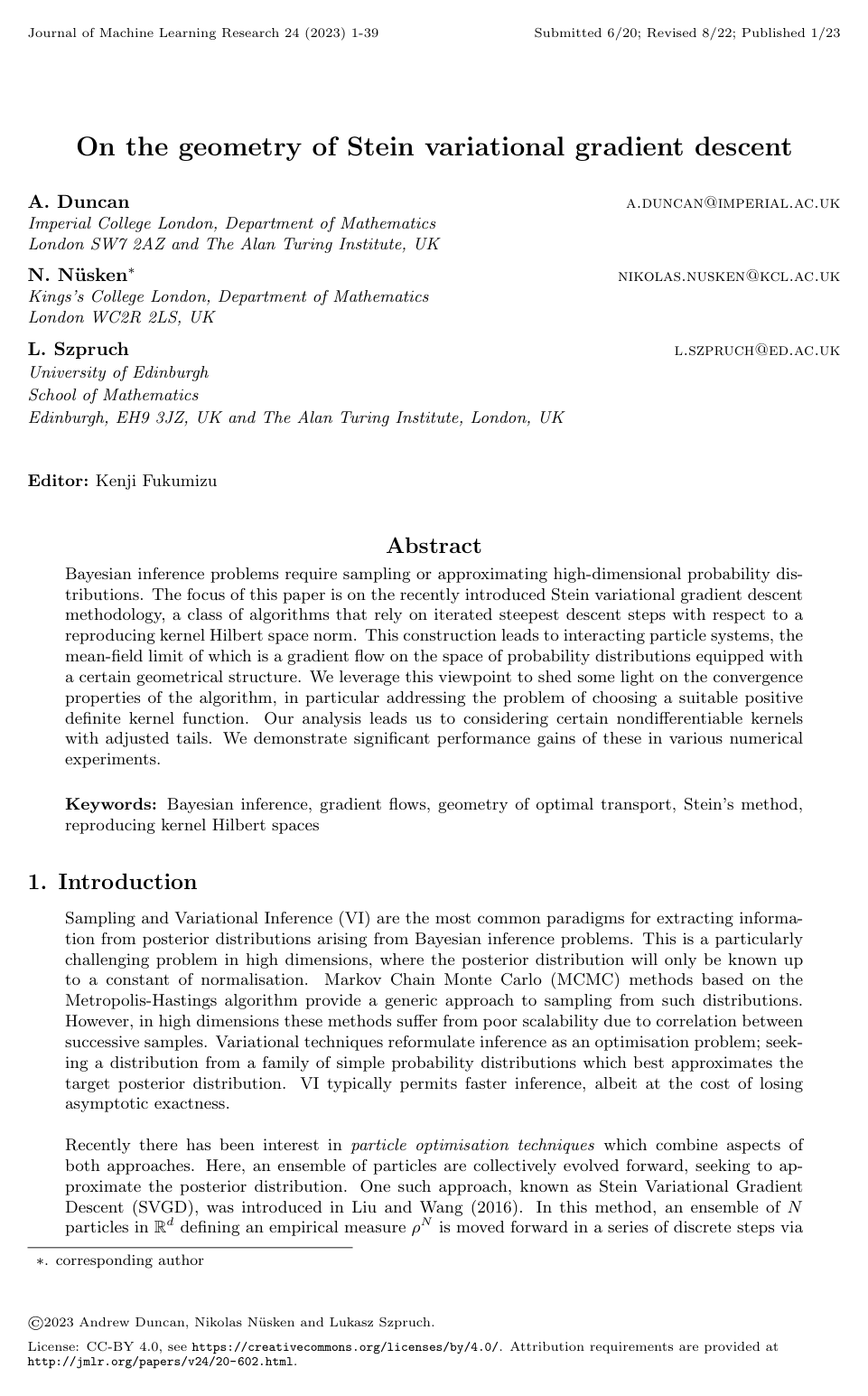
Bayesian inference problems require sampling or approximating high-dimensional probability distributions. The focus of this paper is on the recently introduced Stein variational gradient descent methodology, a class of algorithms that rely on iterated steepest descent steps with respect to a reproducing kernel Hilbert space norm. This construction leads to interacting particle systems, the mean-field limit of which is a gradient flow on the space of probability distributions equipped with a certain geometrical structure. We leverage this viewpoint to shed some light on the convergence properties of the algorithm, in particular addressing the problem of choosing a suitable positive definite kernel function. Our analysis leads us to considering certain nondifferentiable kernels with adjusted tails. We demonstrate significant performance gains of these in various numerical experiments.

Topics

geometry

Keywords

Stein variational gradient descent Stein geometry gradient flows Wasserstein geometry optimal transport Fokker-Planck equation geodesic convexity Langevin dynamics particle optimization quadratic Wasserstein distance

1. Introduction
1.1 Previous work
1.2 Our contribution
2. Assumptions and Preliminaries
2.1 Notation and preliminaries
3. Stochastic SVGD and its Mean Field Limit
4. SVGD as a gradient flow
5. Second order calculus for SVGD
6. Curvature at equilibrium
6.1 The one-dimensional case
7. Outlook: polynomial kernels
8. Numerical Experiments
9. Conclusions
Appendix A. Analogies between Langevin dynamics and SVGD
A.1 Overdamped Langevin dynamics, the Fokker-Planck equation and optimal transport
Appendix B. Proofs for Section 3
Appendix C. Proofs for Section 4
Appendix D. Proofs for Section 5
Appendix E. Proof of Lemma 25
Appendix F. Proofs for Section 6
References

Knowls

Knowl 1 — Riemannian Stein Geometry on Probability Densities
definition
Let $\mathcal{P}_k(\mathbb{R}^d)$ denote the space of probability measures $\rho$ on $\mathbb{R}^d$ admitting a smooth Lebesgue density with full support $\mathrm{supp}\,\rho = \mathbb{R}^d$ and satisfying $\int_{\mathbb{R}^d} k(x, x)\,\rho(x)\,dx < \infty$ , where $k: \mathbb{R}^d \times \mathbb{R}^d \to \mathbb{R}$ is a continuous, symmetric, and integrally strictly positive definite (ISPD) kernel. Let $\mathcal{H}_k$ be the reproducing kernel Hilbert space (RKHS) associated with $k$ , and let $\mathcal{H}_k^d = \mathcal{H}_k \times \dots \times \mathcal{H}_k$ ( $d$ times) be the Hilbert space of vector fields equipped with norm $\|v\|_{\mathcal{H}_k^d}^2 = \sum_{i=1}^d \|v_i\|_{\mathcal{H}_k}^2$ .

For $\rho \in \mathcal{P}_k(\mathbb{R}^d)$ , define the integral operator $\mathcal{T}_{k,\rho}: L^2(\rho) \to \mathcal{H}_k$ by

$\mathcal{T}_{k,\rho}\phi = \int_{\mathbb{R}^d} k(\cdot, y)\,\phi(y)\,\rho(y)\,dy.$

The tangent space $T_\rho \mathcal{P}_k(\mathbb{R}^d)$ at $\rho$ is defined by

$T_\rho \mathcal{P}_k(\mathbb{R}^d) = \left\{ \xi \in \mathcal{D}'(\mathbb{R}^d) : \text{there exists } v \in \overline{\mathcal{T}_{k,\rho}\nabla C_c^\infty(\mathbb{R}^d)}^{\mathcal{H}_k^d} \text{ such that } \xi + \nabla \cdot (\rho v) = 0 \text{ in } \mathcal{D}'(\mathbb{R}^d) \right\},$

and is endowed with the Riemannian metric $g_\rho: T_\rho \mathcal{P}_k(\mathbb{R}^d) \times T_\rho \mathcal{P}_k(\mathbb{R}^d) \to \mathbb{R}$ given by

$g_\rho(\xi, \chi) = \langle u, v \rangle_{\mathcal{H}_k^d},$

where $\xi + \nabla \cdot (\rho u) = 0$ and $\chi + \nabla \cdot (\rho v) = 0$ with $u, v \in \overline{\mathcal{T}_{k,\rho}\nabla C_c^\infty(\mathbb{R}^d)}^{\mathcal{H}_k^d}$ . The space $(T_\rho \mathcal{P}_k(\mathbb{R}^d), g_\rho)$ is a Hilbert space isometrically isomorphic to $(\overline{\mathcal{T}_{k,\rho}\nabla C_c^\infty(\mathbb{R}^d)}^{\mathcal{H}_k^d}, \langle \cdot, \cdot \rangle_{\mathcal{H}_k^d})$ .

Furthermore, $\mathcal{H}_k^d$ admits the $\mathcal{H}_k^d$ -orthogonal Helmholtz decomposition:

$\mathcal{H}_k^d = \left( L_{\mathrm{div}}^2(\rho) \cap \mathcal{H}_k^d \right) \oplus \overline{\mathcal{T}_{k,\rho}\nabla C_c^\infty(\mathbb{R}^d)}^{\mathcal{H}_k^d},$

where $L_{\mathrm{div}}^2(\rho) = \{ v \in (L^2(\rho))^d : \langle v, \nabla \phi \rangle_{(L^2(\rho))^d} = 0 \text{ for all } \phi \in C_c^\infty(\mathbb{R}^d) \}$ is the space of weighted divergence-free vector fields.
Knowl 2 — Stein Gradient Flow Formulation of SVGD
theoretical result
Let $\pi(x) = \frac{1}{Z} e^{-V(x)}$ be a target probability density on $\mathbb{R}^d$ for a continuously differentiable potential $V: \mathbb{R}^d \to \mathbb{R}$ with $e^{-V} \in L^1(\mathbb{R}^d)$ and $\pi \in \mathcal{P}_k(\mathbb{R}^d)$ . For a functional $F: \mathcal{P}_k(\mathbb{R}^d) \to \mathbb{R}$ with $L^2(\mathbb{R}^d)$ -functional derivative $\frac{\delta F}{\delta \rho}(\rho)$ , the Riemannian gradient on $(\mathcal{P}_k(\mathbb{R}^d), g_\rho)$ is given by

$\mathrm{grad}_k F(\rho) = -\nabla \cdot \left( \rho \mathcal{T}_{k,\rho} \nabla \frac{\delta F}{\delta \rho}(\rho) \right),$

where $\mathcal{T}_{k,\rho}\phi(x) = \int_{\mathbb{R}^d} k(x, y)\,\phi(y)\,\rho(y)\,dy$ .

For the Kullback-Leibler divergence $\mathrm{KL}(\rho|\pi) = \int_{\mathbb{R}^d} \rho(x) \log\left(\frac{\rho(x)}{\pi(x)}\right) dx$ , whose functional derivative is $\frac{\delta \mathrm{KL}}{\delta \rho}(\rho) = \log\rho + 1 + V$ , the gradient flow $\partial_t \rho_t = -\mathrm{grad}_k \mathrm{KL}(\rho_t|\pi)$ on the Stein manifold yields the mean-field PDE of Stein Variational Gradient Descent (SVGD):

$\partial_t \rho_t(x) = \nabla \cdot \left( \rho_t(x) \int_{\mathbb{R}^d} k(x, y) [\nabla \rho_t(y) + \rho_t(y) \nabla V(y)] \, dy \right).$

As an immediate consequence of the gradient flow structure, the KL divergence is non-increasing along the solutions: $\frac{d}{dt}\mathrm{KL}(\rho_t | \pi) \le 0$ .
Knowl 3 — Dynamical Stein Distance
definition
For probability measures $\mu, \nu \in \mathcal{P}_k(\mathbb{R}^d)$ , the Stein distance $d_k(\mu, \nu)$ is defined via the Benamou-Brenier type dynamical formulation:

$d_k^2(\mu, \nu) = \inf_{(\rho, v) \in \mathcal{A}(\mu, \nu)} \int_0^1 \|v_t\|_{\mathcal{H}_k^d}^2 \, dt,$

where the set of connecting curves is

$\mathcal{A}(\mu, \nu) = \left\{ (\rho, v) : [0, 1] \to \mathcal{P}_k(\mathbb{R}^d) \times \mathcal{H}_k^d : \rho_0 = \mu, \, \rho_1 = \nu, \, \partial_t \rho + \nabla \cdot (\rho v) = 0 \text{ in } \mathcal{D}'(\mathbb{R}^d) \right\}.$

The infimum in $d_k^2(\mu, \nu)$ is unchanged if $v_t$ is constrained to lie in the subspace $\overline{\mathcal{T}_{k,\rho_t}\nabla C_c^\infty(\mathbb{R}^d)}^{\mathcal{H}_k^d}$ for all $t \in [0, 1]$ .

The Stein distance $d_k$ is an extended metric on $\mathcal{P}_k(\mathbb{R}^d)$ . If the positive definite kernel $k$ is continuous and bounded, $d_k$ dominates the quadratic Wasserstein distance $W_2$ :

$W_2(\mu, \nu) \le C d_k(\mu, \nu) \quad \text{for all } \mu, \nu \in \mathcal{P}_k(\mathbb{R}^d),$

for a constant $C > 0$ , implying that the topology induced by $d_k$ is strictly stronger than weak convergence.
Knowl 4 — Geodesic Equations in Stein Geometry
theoretical result
Let $(\rho_t, v_t)_{0 \le t \le 1}$ be a constant-speed geodesic on $(\mathcal{P}_k(\mathbb{R}^d), d_k)$ , defined as a critical point of the action functional $\int_0^1 \|v_t\|_{\mathcal{H}_k^d}^2 dt$ under the continuity equation constraint. Then $(\rho_t)_{0 \le t \le 1}$ is described by the coupled PDE system for the density $\rho_t$ and a potential function $\Psi: [0, 1] \times \mathbb{R}^d \to \mathbb{R}$ :

$\partial_t \rho_t + \nabla \cdot (\rho_t \mathcal{T}_{k,\rho_t} \nabla \Psi_t) = 0,$

$\partial_t \Psi_t + \nabla \Psi_t \cdot \mathcal{T}_{k,\rho_t} \nabla \Psi_t = 0,$

with velocity field $v_t = \mathcal{T}_{k,\rho_t} \nabla \Psi_t$ , where $\mathcal{T}_{k,\rho_t}\phi = \int_{\mathbb{R}^d} k(\cdot, y)\,\phi(y)\,\rho_t(y)\,dy$ .

In contrast to the geodesic equations for the quadratic Wasserstein distance $W_2$ (where the Hamilton-Jacobi equation $\partial_t \Psi + \frac{1}{2}|\nabla \Psi|^2 = 0$ decouples from the continuity equation), the Stein geodesic equations are mutually coupled due to the non-local density dependence in $\mathcal{T}_{k,\rho_t}$ .
Knowl 5 — Stein-Hessian Operator of the KL Divergence
theoretical result
Let $(\rho_t, \Psi_t)_{t \in (-\varepsilon, \varepsilon)}$ be a smooth Stein geodesic satisfying $\partial_t \rho_t + \nabla \cdot (\rho_t \mathcal{T}_{k,\rho_t} \nabla \Psi_t) = 0$ and $\partial_t \Psi_t + \nabla \Psi_t \cdot \mathcal{T}_{k,\rho_t} \nabla \Psi_t = 0$ with $\rho_0 \equiv \rho$ and $\Psi_0 \equiv \Psi$ . The second derivative of the KL divergence with respect to the target $\pi \propto e^{-V}$ along the geodesic is given by the bilinear form:

$\left. \frac{d^2}{dt^2} \mathrm{KL}(\rho_t | \pi) \right|_{t=0} = \mathrm{Hess}_\rho(\Psi, \Psi) = \sum_{i,j=1}^d \int_{\mathbb{R}^d} \int_{\mathbb{R}^d} \partial_i \Psi(y) \, q_{ij}[\rho](y, z) \, \partial_j \Psi(z) \, \rho(y)\,\rho(z) \, dy \, dz,$

where the kernel tensor $q_{ij}[\rho](y, z)$ decomposes as:

$q_{ij}[\rho](y, z) = \delta_{ij} \sum_{l=1}^d \int_{\mathbb{R}^d} \partial_{x_l} \left( e^{-V(x)} k(x, y) \right) e^{V(x)} \partial_{y_l} k(y, z) \, \rho(x) \, dx$

$- \int_{\mathbb{R}^d} \partial_{y_j} \partial_{x_i} \left( e^{-V(x)} k(x, y) \right) e^{V(x)} k(y, z) \, \rho(x) \, dx$

$- \int_{\mathbb{R}^d} \partial_{x_j} \left( e^{V(x)} \partial_{x_i} \left( e^{-V(x)} k(x, y) \right) \right) k(x, z) \, \rho(x) \, dx.$
Knowl 6 — Non-Convexity of Entropy along Stein Geodesics
theoretical result
Let $\mathrm{Reg}(\rho) = \int_{\mathbb{R}^d} \rho(x) \log\rho(x)\,dx$ denote the negative differential entropy. Unlike in Wasserstein geometry where $\mathrm{Reg}(\rho)$ is displacement convex along geodesics, in Stein geometry $\mathrm{Reg}(\rho)$ is strictly non-convex along linear test directions for any translation-invariant kernel:

Let $\Psi: \mathbb{R}^d \to \mathbb{R}$ be a non-zero linear function $\Psi(x) = a \cdot x$ with $a \in \mathbb{R}^d \setminus \{0\}$ , let $k(x, y) = h(x - y)$ be any integrally strictly positive definite translation-invariant kernel, and let $\rho \in \mathcal{P}_k(\mathbb{R}^d)$ . Then the entropic contribution to the Stein Hessian satisfies

$\mathrm{Hess}_\rho^{\mathrm{Reg}}(\Psi, \Psi) = -\sum_{i,l=1}^d a_i^2 \int_{\mathbb{R}^d} \left( \int_{\mathbb{R}^d} k(x, y)\,\partial_{x_l}\rho(x)\,dx \right)^2 \rho(y)\,dy < 0.$

Consequently, the entropic regularisation alone cannot guarantee geodesic convexity or exponential decay in Stein geometry.
Knowl 7 — Curvature at Equilibrium and the Stein-Poincaré Inequality
theoretical result
Let $\pi(x) \propto e^{-V(x)}$ and let $k$ be an integrally strictly positive definite (ISPD) kernel. At equilibrium $\rho = \pi$ , the Hessian tensor simplifies to

$q_{ij}[\pi](y, z) = \int_{\mathbb{R}^d} \partial_i \partial_j V(x) k(x, y) k(x, z) \pi(x) \, dx + \int_{\mathbb{R}^d} \partial_{x_i} k(x, z) \partial_{x_j} k(x, y) \pi(x) \, dx.$

For any $\lambda \ge 0$ , the following two statements are equivalent:
1. The local exponential decay condition holds:
$\mathrm{Hess}_\pi(\Psi, \Psi) \ge \lambda \int_{\mathbb{R}^d} \int_{\mathbb{R}^d} \nabla \Psi(y) \cdot k(y, z) \nabla \Psi(z) \pi(y) \pi(z) \, dy \, dz \quad \text{for all } \Psi \in C_c^\infty(\mathbb{R}^d).$
1. The Stein-Poincaré inequality holds:
$\langle \phi, \mathcal{L}\phi \rangle_{L^2(\pi)} \ge \lambda \langle \phi, \phi \rangle_{L^2(\pi)} \quad \text{for all } \phi \in L^2_0(\pi) \cap C_c^\infty(\mathbb{R}^d),$

where $L^2_0(\pi) = \{ \phi \in L^2(\pi) : \int_{\mathbb{R}^d} \phi\,d\pi = 0 \}$ , and $\mathcal{L}$ is the symmetric positive semi-definite operator on $L^2(\pi)$ defined by

$\mathcal{L}\phi = -\sum_{i=1}^d e^V \partial_i \left( e^{-V} \mathcal{T}_{k,\pi} \partial_i \phi \right).$

The optimal local decay rate is given by the spectral gap $\lambda = \inf(\sigma(\mathcal{L}) \setminus \{0\})$ .
Knowl 8 — Impossibility of Exponential Convergence Near Equilibrium for Smooth Kernels
theoretical result
Let $k \in C^{1,1}(\mathbb{R}^d \times \mathbb{R}^d)$ and assume the integrability condition

$\sum_{i=1}^d \int_{\mathbb{R}^d} \left[ (\partial_i V(x))^2 k(x, x) - \partial_i V(x) \left( \partial_i^1 k(x, x) + \partial_i^2 k(x, x) \right) + \partial_i^1 \partial_i^2 k(x, x) \right] \pi(x) \, dx < \infty,$

where $\partial_i^1$ and $\partial_i^2$ denote partial derivatives with respect to the $i$ -th component of the first and second arguments of $k$ , respectively.

Under this condition, the operator $\mathcal{L} = -\sum_{i=1}^d e^V \partial_i \left( e^{-V} \mathcal{T}_{k,\pi} \partial_i \cdot \right)$ is compact on $L^2(\pi)$ . By the spectral theorem for compact self-adjoint operators, its spectrum consists of eigenvalues $\mu_i \to 0$ . Therefore, the Stein-Poincaré inequality and local exponential decay condition near equilibrium hold only for $\lambda = 0$ .

Consequently, exponential convergence of SVGD to equilibrium is impossible for smooth kernels such as the Gaussian kernel.
Knowl 9 — One-Dimensional Criterion and Failure of Translation-Invariant Kernels
theoretical result
In dimension $d = 1$ , let $\mathcal{H}_k \subseteq H^1(\pi)$ with dense embedding, and let $V \in C^2(\mathbb{R})$ have bounded second derivative. For $\lambda > 0$ , local exponential decay near equilibrium holds if and only if

$\int_{\mathbb{R}} V''(x) \phi(x)^2 \pi(x) \, dx + \int_{\mathbb{R}} (\phi'(x))^2 \pi(x) \, dx \ge \lambda \|\phi\|_{\mathcal{H}_k}^2 \quad \text{for all } \phi \in \mathcal{H}_k.$

If $k$ is translation-invariant ( $k(x, y) = h(x - y)$ with $h \in C(\mathbb{R}) \cap C^1(\mathbb{R} \setminus \{0\})$ absolutely continuous) and satisfies vanishing tails $h(x) \to 0$ and $h'(x) \to 0$ as $x \to \pm\infty$ , then testing with $\phi_x = h(x - \cdot) \in \mathcal{H}_k$ as $x \to \pm\infty$ yields a left-hand side tending to $0$ while $\|\phi_x\|_{\mathcal{H}_k}^2 = h(0) > 0$ .

Thus, exponential convergence near equilibrium cannot hold (forcing $\lambda = 0$ ) for any standard translation-invariant kernel in 1D.
Knowl 10 — Exponential Convergence Near Equilibrium via Weighted Matérn Kernels
theoretical result
In dimension $d = 1$ , consider the non-differentiable, tail-weighted kernel

$k(x, y) = \pi(x)^{-1/2} e^{-|x - y|} \pi(y)^{-1/2},$

where $\pi(x) \propto e^{-V(x)}$ is the target density. The RKHS associated with $k$ is $\mathcal{H}_k = \{ \pi^{-1/2} f : f \in H^1(\mathbb{R}) \}$ with inner product $\langle \pi^{-1/2} f, \pi^{-1/2} f \rangle_{\mathcal{H}_k} = \|f\|_{H^1(\mathbb{R})}^2 = \int_{\mathbb{R}} [f(x)^2 + (f'(x))^2] dx$ .

If the potential $V \in C^2(\mathbb{R})$ satisfies

$V''(x) + \frac{(V'(x))^2}{2} \ge \tilde{\lambda} > 0 \quad \text{for all } x \in \mathbb{R},$

then exponential convergence near equilibrium holds with explicit rate

$\lambda = \min\left(1, \frac{\tilde{\lambda}}{2}\right) > 0.$

This proves that non-differentiability and tail weighting can overcome the zero-spectral-gap obstruction of smooth, translation-invariant kernels.
Knowl 11 — RKHS Inclusion and Dominance for Fractional Power Exponential Kernels
theoretical result
Consider the family of positive definite kernels $k_{p,\sigma}: \mathbb{R}^d \times \mathbb{R}^d \to \mathbb{R}$ parameterized by smoothness $p \in (0, 2]$ and width $\sigma > 0$ :

$k_{p,\sigma}(x, y) = \exp\left( -\frac{|x - y|^p}{\sigma^p} \right).$
1. $k_{p,\sigma}$ is integrally strictly positive definite (ISPD) for all $p \in (0, 2]$ and $\sigma > 0$ .
2. For any $p > q$ , the RKHSs satisfy the strict inclusion $\mathcal{H}_{k_{p,\sigma_p}} \subsetneq \mathcal{H}_{k_{q,\sigma_q}}$ for all $\sigma_p, \sigma_q > 0$ .
3. For any $p > q$ , there exist bandwidths $\sigma_p, \sigma_q > 0$ such that $\|\phi\|_{\mathcal{H}_{k_{q,\sigma_q}}} \le \|\phi\|_{\mathcal{H}_{k_{p,\sigma_p}}}$ for all $\phi \in \mathcal{H}_{k_{p,\sigma_p}}$ .
In terms of the Rayleigh coefficient $\lambda_\Psi^k = \frac{\mathrm{Hess}_\pi(\Psi, \Psi)}{\int\int \nabla \Psi(y) \cdot k(y, z) \nabla \Psi(z) \pi(y)\pi(z) dy dz}$ , smaller values of $p$ reduce the RKHS norm in the denominator, allowing less regular kernels ( $p=1$ Laplace or $p=0.5$ ) to locally dominate smoother kernels ( $p=2$ Gaussian).
Knowl 12 — Ergodicity of Stochastic SVGD Particle Dynamics
theoretical result
For an ensemble of $N$ particles $\bar{X}_t = (X_t^1, \dots, X_t^N) \in \mathbb{R}^{Nd}$ and potential $\bar{V}(\bar{x}) = \sum_{i=1}^N V(x_i)$ , stochastic SVGD dynamics are defined by the SDE

$dX_t^i = \frac{1}{N} \sum_{j=1}^N \left[ -k(X_t^i, X_t^j) \nabla V(X_t^j) + \nabla_{X_t^j} k(X_t^i, X_t^j) \right] dt + \sum_{j=1}^N \left( \sqrt{2\mathcal{K}(\bar{X}_t)} \right)_{ij} dW_t^j,$

where $\mathcal{K}(\bar{x}) \in \mathbb{R}^{Nd \times Nd}$ is block-structured with blocks $\mathcal{K}_{ij}(\bar{x}) = \frac{1}{N} k(x_i, x_j) I_{d \times d}$ , and $W_t$ is an $Nd$ -dimensional Brownian motion.

Assume $d \ge 2$ , that $V$ satisfies suitable growth conditions, and that $k(x, y) = h(x - y)$ is translation-invariant with $h \in C(\mathbb{R}^d) \cap C^1(\mathbb{R}^d \setminus \{0\})$ Lipschitz continuous satisfying the one-sided condition $(\nabla h(x) - \nabla h(y)) \cdot (x - y) \le C|x - y|^2$ for all $x, y \ne 0$ . If the initial particles are distinct ( $X_0^i \ne X_0^j$ for $i \ne j$ ), then particles never collide ( $X_t^i \ne X_t^j$ almost surely for all $t > 0$ ), and the system is ergodic with unique invariant measure given by the product density

$\bar{\pi}(x_1, \dots, x_N) = \prod_{i=1}^N \pi(x_i) = \frac{1}{Z^N} \exp\left( -\sum_{i=1}^N V(x_i) \right).$

In the mean-field limit $N \to \infty$ , the noise term vanishes and the empirical measure $\rho_t^N = \frac{1}{N}\sum_{i=1}^N \delta_{X_t^i}$ converges to the deterministic mean-field Stein PDE.
Knowl 13 — Empirical Performance of Non-Smooth Kernels and Annealing in SVGD
empirical result
Numerical simulations of SVGD with $N = 500$ particles on 1D and 2D Gaussian mixture models using kernels $k_{p,\sigma}(x, y) = \exp(-|x - y|^p / \sigma^p)$ with bandwidth $\sigma$ chosen via the median heuristic show:
1. Reducing kernel smoothness from $p = 2$ (Gaussian) to $p = 1$ (Laplace) or $p = 0.5$ dramatically reduces the finite-particle bias and lowers the Wasserstein-1 error ( $W_1$ ) to the target distribution, yielding more efficient particle packing.
2. For $p < 1$ , the derivative of the kernel becomes singular at the origin ( $|x - y| \to 0$ ), making the particle ODE system numerically stiff. When integrated with implicit variable-order backward differentiation formula (BDF) schemes, computational cost per unit time rises sharply, and performance degrades for $p \le 0.1$ .
3. A geometric annealing schedule for the smoothness parameter, $\log p(t) = (1 - t/T) \log p_0 + (t/T) \log p_1$ from $p_0 = 2$ down to $p_1 = 0.5$ over simulation window $T$ , achieves the lowest overall $W_1$ error at intermediate times and per gradient evaluation.
Knowl 14 — Contraction of Stein Hessian for Quadratic Potentials with Linear Kernels
theoretical result
In dimension $d = 1$ , let the target potential be quadratic $V(x) = \frac{\alpha}{2} x^2$ with $\alpha > 0$ , and consider the polynomial kernel $k(x, y) = xy$ . Then the tensor $q[\rho](y, z)$ of the Stein-Hessian simplifies to

$q[\rho](y, z) = 2\alpha k(y, z) \int_{\mathbb{R}} x^2 \, \rho(x) \, dx,$

which implies that the Stein-Hessian satisfies

$\mathrm{Hess}_\rho(\Psi, \Psi) \ge \lambda \int_{\mathbb{R}} \int_{\mathbb{R}} \Psi'(y) k(y, z) \Psi'(z) \, \rho(y)\rho(z) \, dy \, dz,$

with contraction rate

$\lambda = 2\alpha \int_{\mathbb{R}} x^2 \, \rho(x) \, dx.$

Thus, whenever $\rho \ne \delta_0$ , $\lambda > 0$ , and the rate of contraction is directly governed by the target curvature $\alpha$ and the second moment of the current distribution $\rho$ .

Coverage note — None was omitted; all central theoretical results, geometric constructions, functional inequalities, kernel comparison theorems, and experimental conclusions have been covered.

References

1.L. Ambrogioni, U. Guclu, Y. Gucluturk, and M. van Gerven. Wasserstein variational gradient descent: From semi-discrete optimal transport to ensemble variational inference. arXiv:1811.02827, 2018.
2.L. Ambrosio and N. Gigli. A user’s guide to optimal transport. In Modelling and optimisation of flows on networks, pages 1–155. Springer, 2013.
3.L. Ambrosio, N. Gigli, and G. Savar´e. Gradient flows: in metric spaces and in the space of probability measures. Springer Science & Business Media, 2008.
4.M. Arbel, A. Korba, A. Salim, and A. Gretton. Maximum mean discrepancy gradient flow. In Advances in Neural Information Processing Systems 32, 2019.
5.S. Arnrich, A. Mielke, M. A. Peletier, G. Savar´e, and M. Veneroni. Passing to the limit in a Wasserstein gradient flow: from diffusion to reaction. Calculus of Variations and Partial Differential Equations, 44 (3-4):419–454, 2012.
6.D. Bakry, I. Gentil, and M. Ledoux. Analysis and geometry of Markov diffusion operators, volume 348. Springer Science & Business Media, 2013.
7.J.-D. Benamou and Y. Brenier. A computational fluid mechanics solution to the Monge-Kantorovich mass transfer problem. Numerische Mathematik, 84(3):375–393, 2000.
8.D. Bigoni, O. Zahm, A. Spantini, and Y. Marzouk. Greedy inference with layers of lazy maps. arXiv:1906.00031, 2019.
9.F. Bolley, D. Chafa¨ı, J. Fontbona, et al. Dynamics of a planar Coulomb gas. The Annals of Applied Probability, 28(5):3152–3183, 2018.
10.L. Brasco. A survey on dynamical transport distances. Journal of Mathematical Sciences, 181(6):755–781, 2012.
11.G. Buttazzo, C. Jimenez, and E. Oudet. An optimization problem for mass transportation with congested dynamics. SIAM Journal on Control and Optimization, 48(3):1961–1976, 2009.
12.G. D. Byrne and A. C. Hindmarsh. A polyalgorithm for the numerical solution of ordinary differential equations. ACM Transactions on Mathematical Software (TOMS), 1(1):71–96, 1975.
13.C. Carmeli, E. De Vito, and A. Toigo. Vector valued reproducing kernel Hilbert spaces of integrable functions and Mercer theorem. Analysis and Applications, 4(04):377–408, 2006.
14.R. Carmona and F. Delarue. Probabilistic Theory of Mean Field Games with Applications I-II. Springer, 2018.
15.J. A. Carrillo, S. Lisini, G. Savar´e, and D. Slepˇcev. Nonlinear mobility continuity equations and generalized displacement convexity. Journal of Functional Analysis, 258(4):1273–1309, 2010.
16.C. Chen and R. Zhang. Particle optimization in MCMC. arXiv:1711.10927, 2017.
17.C. Chen, R. Zhang, W. Wang, B. Li, and L. Chen. A unified particle-optimization framework for scalable Bayesian sampling. In Proceedings of the Thirty-Fourth Conference on Uncertainty in Artificial Intelligence, UAI. AUAI Press, 2018a.
18.P. Chen, K. Wu, J. Chen, T. O’Leary-Roseberry, and O. Ghattas. Projected Stein variational Newton: A fast and scalable Bayesian inference method in high dimensions. In Advances in Neural Information Processing Systems 32, 2019.
19.W. Y. Chen, L. Mackey, J. Gorham, F.-X. Briol, and C. Oates. Stein points. In International Conference on Machine Learning, pages 844–853. PMLR, 2018b.
20.S. Daneri and G. Savar´e. Eulerian calculus for the displacement convexity in the Wasserstein distance. SIAM Journal on Mathematical Analysis, 40(3):1104–1122, 2008.
21.G. Detommaso, T. Cui, Y. Marzouk, A. Spantini, and R. Scheichl. A Stein variational Newton method. In Advances in Neural Information Processing Systems 31, 2018.
22.G. Detommaso, H. Hoitzing, T. Cui, and A. Alamir. Stein variational online changepoint detection with applications to Hawkes processes and neural networks. arXiv:1901.07987, 2019.
23.J. Dolbeault, B. Nazaret, and G. Savar´e. A new class of transport distances between measures. Calculus of Variations and Partial Differential Equations, 34(2):193–231, 2009.
24.A. B. Duncan, N. N¨usken, and G. A. Pavliotis. Using perturbed underdamped Langevin dynamics to efficiently sample from probability distributions. J. Stat. Phys., 169(6):1098–1131, 2017. ISSN 0022-4715. URL https://doi.org/10.1007/s10955-017-1906-8.
25.G. E. Fasshauer. Meshfree approximation methods with MATLAB, volume 6. World Scientific, 2007.
26.Alessio Figalli and Federico Glaudo. An Invitation to Optimal Transport, Wasserstein Distances, and Gradient Flows. EMS Press, 2021.
27.R. Flamary and N. Courty. POT python optimal transport library, 2017.
28.K. Fukumizu, A. Gretton, G. R. Lanckriet, B. Sch¨olkopf, and B. K. Sriperumbudur. Kernel choice and classifiability for RKHS embeddings of probability distributions. In Advances in neural information processing systems, pages 1750–1758, 2009.
29.V. Gallego and D. R. Insua. Stochastic gradient MCMC with repulsive forces. arXiv:1812.00071, 2018.
30.Y. Gao, Y. Jiao, Y. Wang, Y. Wang, C. Yang, and S. Zhang. Deep generative learning via variational gradient flow. In International Conference on Machine Learning, pages 2093–2101. PMLR, 2019.
31.A. Garbuno-Inigo, N. N¨usken, and S. Reich. Affine invariant interacting Langevin dynamics for Bayesian inference. SIAM Journal on Applied Dynamical Systems, 19(3):1633–1658, 2020a.
32.Alfredo Garbuno-Inigo, Franca Hoffmann, Wuchen Li, and Andrew M Stuart. Interacting langevin diffusions: Gradient structure and ensemble kalman sampler. SIAM Journal on Applied Dynamical Systems, 19(1): 412–441, 2020b.
33.N. Gigli. Second Order Analysis on (P2(M), W2). American Mathematical Soc., 2012.
34.M. A. Iglesias, K. J. H. Law, and A. M. Stuart. Ensemble Kalman methods for inverse problems. Inverse Problems, 29(4):045001, 2013.
35.R. Jordan, D. Kinderlehrer, and F. Otto. The variational formulation of the Fokker–Planck equation. SIAM journal on mathematical analysis, 29(1):1–17, 1998.
36.Ansgar J¨ungel. Entropy methods for diffusive partial differential equations, volume 804. Springer, 2016.
37.R Khasminskii. Stochastic stability of differential equations, volume 66. Springer Science & Business Media, 2011.
38.W. Kliemann. Recurrence and invariant measures for degenerate diffusions. The Annals of Probability, pages 690–707, 1987.
39.A. Koldobsky. Fourier analysis in convex geometry. Number 116. American Mathematical Soc., 2005.
40.E. Kreyszig. Introductory functional analysis with applications, volume 1. Wiley New York, 1978.
41.J. M. Lee. Riemannian manifolds: an introduction to curvature, volume 176. Springer Science & Business Media, 2006.
42.L. Li, Y. Li, J.-G. Liu, Z. Liu, and J. Lu. A stochastic version of Stein variational gradient descent for efficient sampling. Communications in Applied Mathematics and Computational Science, 15(1):37–63, 2020.
43.W. Li. Diffusion hypercontractivity via generalized density manifold. arXiv preprint arXiv:1907.12546, 2019.
44.W. Li. Hessian metric via transport information geometry. Journal of Mathematical Physics, 62(3):033301, 2021.
45.W. Li and G. Mont´ufar. Natural gradient via optimal transport. Information Geometry, 1(2):181–214, 2018.
46.W. Li and G. Mont´ufar. Ricci curvature for parametric statistics via optimal transport. Information Geometry, 3(1):89–117, 2020.
47.M. Liero and A. Mielke. Gradient structures and geodesic convexity for reaction–diffusion systems. Philosophical Transactions of the Royal Society A: Mathematical, Physical and Engineering Sciences, 371(2005): 20120346, 2013.
48.C. Liu and J. Zhu. Riemannian Stein variational gradient descent for Bayesian inference. In Thirty-Second AAAI Conference on Artificial Intelligence, 2018.
49.C. Liu, J. Zhuo, P. Cheng, R. Zhang, and J. Zhu. Understanding and accelerating particle-based variational inference. In International Conference on Machine Learning, pages 4082–4092, 2019.
50.Q. Liu. Stein variational gradient descent as gradient flow. In Advances in neural information processing systems, pages 3115–3123, 2017.
51.Q. Liu and D. Wang. Stein variational gradient descent: a general purpose Bayesian inference algorithm. In Advances In Neural Information Processing Systems, pages 2378–2386, 2016.
52.Q. Liu and D. Wang. Stein variational gradient descent as moment matching. In Advances in Neural Information Processing Systems, pages 8868–8877, 2018.
53.A. Liutkus, U. Simsekli, S. Majewski, A. Durmus, and F.-R. St¨oter. Sliced-Wasserstein flows: Nonparametric generative modeling via optimal transport and diffusions. In International Conference on Machine Learning, pages 4104–4113. PMLR, 2019.
54.J. Lott. Some geometric calculations on Wasserstein space. Communications in Mathematical Physics, 277 (2):423–437, 2008.
55.J. Lu, Y. Lu, and J. Nolen. Scaling limit of the Stein variational gradient descent: the mean field regime. SIAM Journal on Mathematical Analysis, 51(2):648–671, 2019a.
56.Y. Lu, J. Lu, and J. Nolen. Accelerating Langevin sampling with birth-death. arXiv:1905.09863, 2019b.
57.Y.-A. Ma, T. Chen, and E. Fox. A complete recipe for stochastic gradient MCMC. In Advances in Neural Information Processing Systems, pages 2899–2907, 2015.
58.S. Machlup and L. Onsager. Fluctuations and irreversible process. ii. systems with kinetic energy. Physical Review, 91(6):1512, 1953.
59.R. J. McCann. A convexity principle for interacting gases. Advances in mathematics, 128(1):153–179, 1997.
60.S. P. Meyn and R. L. Tweedie. Stability of Markovian processes iii: Foster–Lyapunov criteria for continuous-time processes. Advances in Applied Probability, 25(3):518–548, 1993.
61.C. A. Micchelli and M. Pontil. On learning vector-valued functions. Neural computation, 17(1):177–204, 2005.
62.A. Mielke. A gradient structure for reaction–diffusion systems and for energy-drift-diffusion systems. Nonlinearity, 24(4):1329, 2011.
63.A. Mielke. Thermomechanical modeling of energy-reaction-diffusion systems, including bulk-interface interactions. Discr. Cont. Dynam. Systems Ser. S, 6(2):479–499, 2013.
64.A. Mielke, M. A. Peletier, and D. R. M. Renger. On the relation between gradient flows and the large-deviation principle, with applications to Markov chains and diffusion. Potential Analysis, 41(4):1293–1327, 2014.
65.A. Mielke, D. R. M. Renger, and M. A. Peletier. A generalization of Onsager’s reciprocity relations to gradient flows with nonlinear mobility. Journal of Non-Equilibrium Thermodynamics, 41(2):141–149, 2016.
66.Y. Mroueh, C.-L. Li, T. Sercu, A. Raj, and Y. Cheng. Sobolev GAN. In 6th International Conference on Learning Representations, ICLR, 2018.
67.Y. Mroueh, T. Sercu, and A. Raj. Sobolev descent. In The 22nd International Conference on Artificial Intelligence and Statistics, pages 2976–2985, 2019.
68.N. N¨usken and G. A. Pavliotis. Constructing sampling schemes via coupling: Markov semigroups and optimal transport. SIAM/ASA Journal on Uncertainty Quantification, 7(1):324–382, 2019.
69.N. N¨usken and S Reich. Note on interacting Langevin diffusions: Gradient structure and ensemble Kalman sampler by Garbuno-Inigo, Hoffmann, Li and Stuart. arXiv:1908.10890, 2019.
70.N. N¨usken and D. R. Renger. Stein variational gradient descent: many-particle and long-time asymptotics. arXiv preprint arXiv:2102.12956, 2021.
71.H. C. Ottinger. Beyond equilibrium thermodynamics. John Wiley & Sons, 2005.
72.F. Otto. Dynamics of labyrinthine pattern formation in magnetic fluids: A mean-field theory. Archive for Rational Mechanics and Analysis, 141(1):63–103, 1998.
73.F. Otto. The geometry of dissipative evolution equations: the porous medium equation. Communications in Partial Differential Equations, 26(1-2):101–174, 2001.
74.F. Otto and C. Villani. Generalization of an inequality by Talagrand and links with the logarithmic Sobolev inequality. Journal of Functional Analysis, 173(2):361–400, 2000.
75.F. Otto and M. Westdickenberg. Eulerian calculus for the contraction in the Wasserstein distance. SIAM journal on mathematical analysis, 37(4):1227–1255, 2005.
76.S. Pathiraja and S. Reich. Discrete gradients for computational Bayesian inference. Journal of Computational Dynamics, 6(2):385–400, 2019.
77.G. A. Pavliotis. Stochastic processes and applications: Diffusion Processes, the Fokker-Planck and Langevin Equations, volume 60. Springer, 2014.
78.M. A. Peletier. Variational modelling: Energies, gradient flows, and large deviations. arXiv:1402.1990, 2014.
79.M. Pulido and P. J. van Leeuwen. Kernel embedding of maps for sequential Bayesian inference: the variational mapping particle filter. arXiv:1805.11380, 2018.
80.Michael Reed, Barry Simon, Barry Simon, and Barry Simon. Methods of modern mathematical physics, volume 1. Elsevier, 1972.
81.S. Reich and S. Weissmann. Fokker–Planck particle systems for Bayesian inference: Computational approaches. SIAM/ASA Journal on Uncertainty Quantification, 9(2):446–482, 2021.
82.C. Robert and G. Casella. Monte Carlo statistical methods. Springer Science & Business Media, 2013.
83.G. O. Roberts, R. L. Tweedie, et al. Exponential convergence of Langevin distributions and their discrete approximations. Bernoulli, 2(4):341–363, 1996.
84.R. T. Rockafellar. Convex analysis, volume 28. Princeton university press, 1970.
85.S. Saitoh and Y. Sawano. Theory of reproducing kernels and applications. Springer, 2016.
86.B. K. Sriperumbudur, A. Gretton, K. Fukumizu, B. Sch¨olkopf, and G. R. G. Lanckriet. Hilbert space embeddings and metrics on probability measures. Journal of Machine Learning Research, 11(Apr):1517– 1561, 2010.
87.B. K. Sriperumbudur, K. Fukumizu, and G. R. G. Lanckriet. Universality, characteristic kernels and RKHS embedding of measures. Journal of Machine Learning Research, 12(Jul):2389–2410, 2011.
88.I. Steinwart and A. Christmann. Support vector machines. Springer Science & Business Media, 2008.
89.C. Villani. Topics in optimal transportation, volume 58 of Graduate Studies in Mathematics. American Mathematical Society, Providence, RI, 2003a. ISBN 0-8218-3312-X. URL https://doi.org/10.1007/b12016.
90.C. Villani. Optimal transportation, dissipative PDE’s and functional inequalities. In Optimal transportation and applications, pages 53–89. Springer, 2003b.
91.C. Villani. Optimal transport, volume 338 of Grundlehren der Mathematischen Wissenschaften [Fundamental Principles of Mathematical Sciences]. Springer-Verlag, Berlin, 2009. ISBN 978-3-540-71049-3. URL https://doi.org/10.1007/978-3-540-71050-9. Old and new.
92.D. Wang, Z. Tang, C. Bajaj, and Q. Liu. Stein variational gradient descent with matrix-valued kernels. In Advances in Neural Information Processing Systems, pages 7834–7844, 2019a.
93.Y. Wang and W. Li. Information Newton’s flow: second-order optimization method in probability space. arXiv preprint arXiv:2001.04341, 2020.
94.Z. Wang, T. Ren, J. Zhu, and B. Zhang. Function space particle optimization for Bayesian neural networks. In 7th International Conference on Learning Representations, ICLR, 2019b.
95.H. Wendland. Scattered data approximation, volume 17. Cambridge university press, 2004.
96.H. Zhang and L. Zhao. On the inclusion relation of reproducing kernel Hilbert spaces. Analysis and Applications, 11(02):1350014, 2013.
97.J. Zhang, R. Zhang, and C. Chen. Towards more theoretically-grounded sampling for deep learning. openreview.net, 2018.
98.J. Zhang, R. Zhang, L. Carin, and C. Chen. Stochastic particle-optimization sampling and the non-asymptotic convergence theory. In International Conference on Artificial Intelligence and Statistics, pages 1877–1887. PMLR, 2020.
99.J. Zhuo, C. Liu, J. Shi, J. Zhu, N. Chen, and B. Zhang. Message passing Stein variational gradient descent. In International Conference on Machine Learning, pages 6018–6027. PMLR, 2018.

Citation

MLA

Duncan, A., et al. “On the Geometry of Stein Variational Gradient Descent”. Journal of Machine Learning Research, vol. 24, no. 56, 2023, pp. 1–9, https://www.jmlr.org/papers/v24/20-602.html.

APA

Duncan, A., Nüsken, N., & Szpruch, L. (2023). On the geometry of Stein variational gradient descent. Journal of Machine Learning Research, 24(56), 1–39. https://www.jmlr.org/papers/v24/20-602.html

Chicago

Duncan, A., N. Nüsken, and L. Szpruch. 2023. “On the Geometry of Stein Variational Gradient Descent”. Journal of Machine Learning Research 24 (56): 1–39. https://www.jmlr.org/papers/v24/20-602.html.

Harvard

Duncan, A., Nüsken, N. and Szpruch, L. (2023) “On the geometry of Stein variational gradient descent”, Journal of Machine Learning Research, 24(56), pp. 1–39. Available at: https://www.jmlr.org/papers/v24/20-602.html.

Vancouver

1. Duncan A, Nüsken N, Szpruch L (2023) On the geometry of Stein variational gradient descent. Journal of Machine Learning Research 24:1–39

BibTeX

@article{JMLR:v24:20-602,
  author  = {Andrew Duncan and Nikolas NÃ¼sken and Lukasz Szpruch},
  title   = {On the geometry of Stein variational gradient descent},
  journal = {Journal of Machine Learning Research},
  year    = {2023},
  volume  = {24},
  number  = {56},
  pages   = {1--39},
  url     = {http://jmlr.org/papers/v24/20-602.html}
}

Metadata:DOI registry

Access the Paper

This paper is available from its original source. Click below to access the PDF.

Open PDF

License: https://creativecommons.org/licenses/by/4.0/

On the geometry of Stein variational gradient descent

Abstract

Topics

Keywords

Table of Contents

Knowls

Knowl 1 — Riemannian Stein Geometry on Probability Densities

Knowl 2 — Stein Gradient Flow Formulation of SVGD

Knowl 3 — Dynamical Stein Distance

Knowl 4 — Geodesic Equations in Stein Geometry

Knowl 5 — Stein-Hessian Operator of the KL Divergence

Knowl 6 — Non-Convexity of Entropy along Stein Geodesics

Knowl 7 — Curvature at Equilibrium and the Stein-Poincaré Inequality

Knowl 8 — Impossibility of Exponential Convergence Near Equilibrium for Smooth Kernels

Knowl 9 — One-Dimensional Criterion and Failure of Translation-Invariant Kernels

Knowl 10 — Exponential Convergence Near Equilibrium via Weighted Matérn Kernels

Knowl 11 — RKHS Inclusion and Dominance for Fractional Power Exponential Kernels

Knowl 12 — Ergodicity of Stochastic SVGD Particle Dynamics

Knowl 13 — Empirical Performance of Non-Smooth Kernels and Annealing in SVGD

Knowl 14 — Contraction of Stein Hessian for Quadratic Potentials with Linear Kernels

References

Citation

BibTeX

Access the Paper