Stochastic Gradient Descent over P2

Maria Oprea $^{*}$ $^{\dagger}$

Qin Li $^{\ddagger}$

Yunan Yang $^{\S}$

$^{*}$ Center for Applied Mathematics, Cornell University, [email protected], corresponding author

$^{\dagger}$ Current address: Institute of Science and Technology Austria (ISTA)

$^{\ddagger}$ Department of Mathematics, University of Wisconsin--Madison, USA, [email protected]

$^{\S}$ Department of Mathematics, Cornell University, USA, [email protected]

Abstract

Stochastic gradient descent (SGD) admits diffusion approximations that replace the complicated randomness of stochastic gradients by Gaussian noise, providing a powerful tool for understanding its dynamics and long-time behavior. We investigate whether an analogous approximation principle holds for optimization over probability measures, where the objective is a functional defined on the Wasserstein space $\mathcal P_2$. The nonlinear geometry and infinite-dimensional nature of $\mathcal P_2$ prevent a direct extension of the classical Euclidean theory. Using Lions differentiability, we lift the problem to a linear Hilbert space, where higher-order differential calculus becomes available. We then construct a Gaussian random-field approximation whose velocity field matches the mean and covariance of the original stochastic gradient. By exploiting this moment matching through higher-order Taylor expansions, we show that the Gaussian approximation captures the SGD dynamics with second-order weak accuracy. Our result provides a rigorous foundation for replacing sample-driven randomness by analytically tractable Gaussian fluctuations in stochastic optimization over probability measures.

Executive Summary: Modern machine learning and statistical modeling increasingly solve optimization problems over entire probability distributions rather than simple parameter vectors, with applications in generative artificial intelligence, Bayesian inference, and mean-field systems. In traditional Euclidean optimization, stochastic gradient descent (SGD) algorithms are widely approximated by continuous diffusion processes driven by Gaussian noise, which makes complex stochastic dynamics analytically tractable. However, extending this diffusion approximation principle to probability distributions has remained a major theoretical challenge due to the infinite-dimensional and non-linear geometry of Wasserstein probability space.

The article establishes a rigorous mathematical foundation for replacing complex, sample-driven randomness with tractable Gaussian fluctuations when optimizing over probability distributions. Specifically, the objective was to demonstrate that a discrete-time Gaussian random-field approximation accurately captures the dynamics of stochastic Wasserstein gradient descent with second-order weak accuracy.

To overcome the non-linear geometry of probability spaces, the authors employed Lions differentiability, lifting distribution functionals onto a linear Hilbert space to enable higher-order differential calculus and Taylor expansions. They constructed an auxiliary discrete-time iteration driven by a Gaussian random field that matches the mean velocity and covariance of the original stochastic gradient. The theoretical weak convergence was analyzed by tracking test observables across backward transition operators, and the findings were validated using numerical simulations on an exactly solvable quadratic benchmark and a state-dependent distribution reconstruction task using up to two million sample paths.

The theoretical analysis proves that the discrepancy between the original stochastic gradient dynamics and its moment-matched Gaussian surrogate is bounded by the square of the step size, yielding second-order weak accuracy. In an exactly solvable benchmark, the global second-order weak error rate was confirmed to be mathematically sharp, driven directly by unmatched third-order moments. Numerical simulations of a state-dependent moment reconstruction task empirically validated this rate, exhibiting a convergence order of approximately 2.014 with overlapping loss trajectories between the original and Gaussian schemes.

These results show that practitioners and researchers can confidently model the complex, non-Gaussian noise of sample-based optimization over probability distributions using analytically simpler Gaussian processes without sacrificing accuracy. This insight reduces theoretical complexity and provides a reliable framework for understanding the behavior, stability, and trajectory properties of advanced distribution-based learning models without needing to simulate full empirical sample variations.

Future work should focus on extending these principles to unbounded domains, active boundary regimes, and continuous-time stochastic partial differential equations on probability spaces. Researchers are also encouraged to investigate whether matching higher-order moments can yield higher-order accuracy schemes. While the findings provide strong confidence within compact domains and smooth objective functionals, caution is advised when applying these approximations to systems with severe boundary constraints or irregular objectives where regular derivative bounds may not hold.

1. Introduction

Section Summary: Stochastic gradient descent uses random sampling to efficiently minimize expected losses in high dimensions, and its behavior is often approximated by continuous stochastic differential equations whose noise arises from Brownian motion rather than data sampling. Extending this framework to optimization over probability distributions, as needed in variational inference and generative modeling, introduces geometric, stochastic, and analytical difficulties that are only partially resolved by Wasserstein gradient-flow ideas. The paper therefore develops a discrete-time theory based on weak approximation arguments to characterize the resulting dynamics without directly constructing a limiting stochastic partial differential equation.

Stochastic gradient descent (SGD) is one of the fundamental algorithms in modern machine learning and large-scale optimization. Given an expected loss

$ \min_{x \in \mathbb{R}^d} F(x):=\mathbb{E}_{\gamma}[f(x,\gamma)], $

SGD generates iterates according to

$ x_{n+1} =x_n -h_n \nabla_x f(x_n,\gamma_n), $

where ${\gamma_n}$ are independent samples and $h_n$ is the step size. Since $\mathbb{E}_{\gamma}\big[\nabla_x f(x,\gamma)\big]=\nabla_x F(x)$, the stochastic gradient provides an unbiased approximation of the exact gradient, and 2 may be viewed as a stochastic counterpart of the classical gradient descent iteration

$ x_{n+1}

x_n

h_n \nabla_x F(x_n). $

Introduced by Robbins and Monro [1], SGD enables efficient optimization in high-dimensional settings and forms the computational backbone of contemporary machine learning [2].

Beyond computational efficiency, the introduced stochasticity plays a crucial role in the success of SGD. The noise introduced through random sampling often improves exploration of the optimization landscape and can lead to superior practical performance compared with deterministic gradient methods. Understanding the effect of this stochasticity has motivated extensive theoretical investigations. One particularly influential viewpoint studies continuous-time limits of SGD. Under suitable scalings, SGD can be approximated by a stochastic differential equation (SDE)

$ \mathrm{d}X_t = - \nabla F(X_t)\mathrm{d}t +\sqrt{2D(t,X_t)},\mathrm{d}W_t,, $

where the diffusivity coefficient $D$ depends on the stochastic gradient noise. This perspective connects optimization with Langevin dynamics, simulated annealing, and Fokker–Planck equations [3, 4, 5, 6, 7], providing analytical tools that have led to a deeper understanding of the behavior of SGD [8].

The connection between Equation 2 and 4 is far from obvious. The randomness in SGD originates from sampling the random variable $\gamma$, whereas the randomness in the SDE is generated by Brownian motion and is therefore Gaussian. These stochastic mechanisms are fundamentally different, and the diffusion process can only be viewed as an approximation of the discrete algorithm. Establishing the validity of such diffusion approximations, and quantifying the associated approximation error, have been the subject of considerable study in stochastic approximation theory and stochastic modified equations; see, for example, [9].

While classical SGD is formulated in finite-dimensional Euclidean spaces, many contemporary problems require optimization over probability distributions. Examples arise in variational inference, Bayesian sampling [10, 11], generative modeling [12, 13], and mean-field systems [14, 15, 16, 17]. In such settings, the optimization variable is no longer a finite-dimensional parameter vector but a probability measure itself. This naturally leads to problems of the form

$ \min_{\rho\in\mathcal P_2(\mathcal X)} E(\rho),,\qquad\text{with}\qquad E(\rho) :=\mathbb{E}\gamma\big[\mathcal E\gamma(\rho)\big],, $

where $\mathcal P_2(\mathcal X)$ denotes the space of probability measures on $\mathcal X$ with finite second moment, $\gamma$ is a random parameter defined on a probability space $(\Gamma,\mathcal F,\mathbb{P})$, and $\mathcal E_\gamma:\mathcal P_2(\mathcal X)\to\mathbb{R}$ is a sample-dependent loss functional. This definition is an analogue of Equation 1.

Extending the SGD-SDE paradigm from Euclidean spaces to probability spaces introduces several additional difficulties. The first is geometric. Unlike $\mathbb{R}^d$, the space $\mathcal P_2(\mathcal X)$ is not linear, and therefore the additive update underlying classical SGD is no longer meaningful. Fortunately, this obstacle has largely been resolved through the development of optimal transport and Wasserstein gradient-flow theory. Following the framework of Ambrosio, Gigli, and Savaré [18], one may endow $\mathcal P_2(\mathcal X)$ with the Wasserstein metric and define gradients and gradient flows for sufficiently regular functionals.

The second difficulty concerns the nature of the stochasticity. In SGD, randomness enters through independent draws of the sample variable $\gamma$ from its underlying distribution, and the resulting stochastic gradient noise is generally non-Gaussian. By contrast, the continuous-time diffusion model is driven by Brownian motion, or, in the probability-space setting, by a Gaussian random field. Thus the two dynamics are expected to differ pathwise. Following the stochastic modified equation perspective of [9], we instead compare the discrete stochastic iteration and its diffusion approximation in a weak sense. This replaces trajectory-wise accuracy by accuracy of expectations against suitable test functionals, for which matching the drift and covariance of the stochastic increments becomes the central requirement.

A third difficulty arises when one attempts to extend the stochastic modified equation framework itself to probability spaces. In the finite-dimensional setting, the work of [9] establishes a continuous-in-time SDE whose weak solutions provide a high-order approximation of the SGD iterates. Repeating the same program in $\mathcal P_2(\mathcal X)$ is considerably more delicate. Since probability measures are inherently infinite-dimensional objects, the corresponding continuous-time limit is no longer an SDE but rather a stochastic partial differential equation (SPDE). Within the Wasserstein gradient-flow framework, a formal derivation suggests an SPDE driven by a Gaussian velocity field whose covariance is determined by the stochastic gradient fluctuations. At present, however, the well-posedness and regularity theory for such dynamics remain largely unresolved. Consequently, rather than constructing the limiting SPDE directly, we develop the theory at the discrete-time level and use weak approximation arguments to characterize the stochastic dynamics.

Combining these observations, we arrive at a natural analogue of SGD on the Wasserstein space $\mathcal P_2(\mathcal X)$. Following the geometric framework of Wasserstein gradient flows, each stochastic realization generates a velocity field through the first variation of the sample-dependent objective. The resulting stochastic update takes the form:

$ \rho_{n+1} = \Bigl(\mathrm{Id} - h u_{\gamma_n}(\cdot,\rho_n) \Bigr)# \rho_n,\quad\text{with}\quad u\gamma(x,\rho):= \nabla_x \frac{\delta\mathcal E_\gamma}{\delta\rho}(\rho)(x),, $

where $(\gamma_n)_{n\ge0}$ are independent samples drawn from $(\Gamma,\mathcal F,\mathbb{P})$ and $#$ denotes the pushforward operator [18]. This iteration is the natural measure-valued analogue of classical SGD. Its relation to deterministic Wasserstein gradient descent mirrors the relation between Equation 2 and 3 in Euclidean optimization.

Likewise, following the stochastic modified equation philosophy of [9], we seek a Gaussian approximation that matches the first two moments of the stochastic velocity field. This leads to the auxiliary iteration:

$ \widetilde{\rho}{n+1}= \left(\mathrm{Id}-hu{\omega_n}(\cdot,\widetilde{\rho}n)\right)# \widetilde{\rho}_n,, $

where, conditional on $\widetilde{\rho}n$, the random field $u{\omega_n}(\cdot,\widetilde{\rho}n)$ is a Gaussian field that share the mean and the covariance with $u{\gamma}$.

The central objective of this work is to establish a rigorous connection between the stochastic iteration Equation 6 and its Gaussian approximation Equation 7. Since the two velocity fields share the same first and second moments, one naturally expects the two dynamics to agree up to second order in the time step. Our main result confirms this intuition. Adopting the weak-approximation framework of [9], we compare the two processes through sufficiently regular observables and prove a second-order weak error estimate. More precisely, for a suitable class of test functionals on $\mathcal P_2(\mathcal X)$, the discrepancy between the two updates is shown to be of order $\mathcal O(h^2)$. As in the classical theory of stochastic modified equations, the associated error bound grows exponentially with the final time.

The proof relies on two key ingredients. The first is the Wasserstein differential calculus developed through Lions derivatives. By lifting functionals on $\mathcal P_2(\mathcal X)$ to an underlying Hilbert space, Lions differentiability provides a convenient framework for defining higher-order derivatives and carrying out the Taylor expansions required for moment matching. The second ingredient is an iterative weak-error representation formula. In the finite-dimensional setting, a related construction was introduced in [9] and plays a crucial role in controlling the accumulation of local approximation errors. A similar mechanism is employed here. As in the Euclidean theory, repeated iterations lead to a progressive loss of regularity of the test functional, which must be compensated through the smoothing properties of the updates themselves.

The remainder of the paper is organized as follows. Section 2 reviews the Wasserstein geometry and Lions differential calculus that form the analytical foundation of our approach. Section 3 introduces the Gaussian approximation and establishes the main weak-convergence results. Section 4 presents numerical experiments illustrating the second-order weak error in both a solvable benchmark and a state-dependent distribution-reconstruction problem. Section 5 concludes with limitations and directions for future work.

2. Mathematical background

Section Summary: This section assembles the core mathematical tools needed to analyze weak convergence of stochastic particle updates. It draws on Wasserstein geometry to frame gradient flows on probability measures, Lions differentiability to enable Taylor expansions of functionals on those measures, and a covariance identity plus suitable test functions to compare stochastic and deterministic fluctuations. The setup assumes a compact convex domain so that all probability measures have finite second moments and can be treated within the Wasserstein space.

This section collects the background material used throughout the weak-convergence analysis. The proof combines four ingredients. Wasserstein geometry provides the gradient-flow structure underlying the stochastic update. Lions differentiability supplies a differential calculus suitable for higher-order Taylor expansions on probability spaces. A covariance identity for bounded bilinear forms allows us to match the second-order fluctuations of the stochastic and Gaussian velocity fields. Finally, we introduce a class of sufficiently regular test functionals on $\mathcal{P}_2(\mathcal{X})$ against which the weak error will be measured.

Throughout the paper, we assume that $\mathcal{X}\subset \mathbb{R}^d$ is compact and convex. We write

$ R_\mathcal{X}:=\sup_{x\in \mathcal{X}}|x|. $

Since $\mathcal{X}$ is compact, every probability measure on $\mathcal{X}$ has finite second moment. Consequently, $\mathcal{P}_2(\mathcal{X})= \mathcal{P}(\mathcal{X})$ are two equivalent sets. We nevertheless retain the notation $\mathcal{P}_2(\mathcal{X})$ to emphasize the Wasserstein geometry.

2.1 Wasserstein gradient flows

The geometric structure of $\mathcal{P}_2(\mathcal{X})$ is induced by the Wasserstein metric. A particularly useful characterization is the Benamou–Brenier dynamic formulation; see ([19], Chapter 8):

$ W_2^2(\mu,\nu) = \inf_{(\mu_t,v_t)} \left{ \int_0^1\int_{\mathcal{X}}|v_t(x)|^2,d\mu_t(x)dt\middle| \partial_t\mu_t+\nabla\cdot(\mu_t v_t)=0,
\mu_0=\mu,
\mu_1=\nu \right}. $

Here, the continuity equation is understood in the weak sense, together with the usual no-flux boundary condition whenever $\mathcal{X}$ has boundary. This formulation highlights the velocity-field representation of transport, which forms the basis of the gradient-flow construction.

A key consequence of the Wasserstein geometry is that sufficiently regular functionals admit a notion of gradient. Let

$ \mathcal{E}: \mathcal{P}_2(\mathcal{X})\to \mathbb{R} $

be a smooth functional. Then its Wasserstein gradient can be expressed through the first variation as

$ \nabla^{W_2}\mathcal{E}(\rho) =-\nabla\cdot\left(\rho\nabla \left. \frac{\delta \mathcal{E}}{\delta\rho} \right|_\rho\right),, $

where $\frac{\delta \mathcal{E}}{\delta\rho}$ denotes the first variation of $\mathcal{E}$; see, for example, ([20], Proposition 2.2). Throughout the paper, we identify the Wasserstein gradient flow as:

$ \partial_t\rho_t=-\nabla^{W_2}\mathcal{E}(\rho_t)= \nabla\cdot \Bigl( \rho_t u(\cdot,\rho_t) \Bigr),,\quad\text{with}\quad u(x,\rho) := \nabla_x \left. \frac{\delta \mathcal{E}}{\delta\rho} \right|_\rho(x),. $

Applying a forward-Euler discretization to this evolution yields the deterministic update

$ \rho_{n+1}=\Bigl( \mathrm{Id}-h u(\cdot,\rho_n) \Bigr)_# \rho_n,. $

Returning to the stochastic optimization problem Equation 5, each realization $\gamma$ gives rise to a sample-dependent functional $\mathcal{E}\gamma$ and therefore $\nabla^{W_2}\mathcal{E}\gamma(\rho)$ gives rise to a corresponding velocity field

$ u_\gamma(\cdot,\rho):=\nabla_x \left. \frac{\delta \mathcal{E}\gamma}{\delta\rho}\right|\rho ,. $

Replacing the deterministic velocity field in the forward-Euler scheme by a single sample realization $u_{\gamma_n}$ yields precisely the stochastic iteration Equation 6.

2.2 Lions differentiability and Taylor expansion

The analysis developed later relies heavily on higher-order Taylor expansions of functionals defined on $\mathcal{P}_2(\mathcal{X})$. While Wasserstein geometry provides a natural notion of gradient, repeatedly differentiating functionals directly on the space of probability measures is considerably less convenient. A powerful alternative is provided by Lions differentiability, which lifts functionals on $\mathcal{P}_2(\mathcal{X})$ to a linear Hilbert space where classical Fréchet calculus becomes available; see [21], ([22], Chapter 5.2), and [23].

Let $(\Theta,\mathcal F_\theta, \mathbb{P}_\theta)$ be a nonatomic probability space, and define

$ \mathbb{H}:=L^2(\Theta, \mathbb{P}\theta; \mathbb{R}^d),,\quad\text{equipped with}\quad \langle X,Y\rangle{\mathbb{H}} := \int_\Theta \langle X(\theta),Y(\theta)\rangle ,d \mathbb{P}_\theta(\theta). $

Since $\mathbb{P}\theta$ is nonatomic, and $\mathcal{X} \subset \mathbb{R}^d$, every measure $\mu\in \mathcal{P}2(\mathcal{X})$ can be realized as the law of some random variable $X\in \mathbb{H}$; see ([24], Theorem 3.18), with $X(\Theta) \subseteq \mathcal{X}$. That is, $\mu =X# \mathbb{P}\theta$. Consequently, a functional

$ G: \mathcal{P}_2(\mathcal{X})\to \mathbb{R} $

can be lifted to a functional on $\mathbb{H}$ by defining

$ \tilde{G}(X) := G(X_# \mathbb{P}_\theta), \qquad X\in \mathbb{H},. $

The key advantage of this construction is that the domain of $\tilde{G}$ is now a Hilbert space, allowing one to deploy the familiar machinery of Fréchet differentiation.

A subtlety arises from the fact that the lift is not unique. Indeed, multiple random variables may induce the same probability measure: $X_1{}# \mathbb{P}\theta= X_2{}# \mathbb{P}\theta$. The lifted functional itself is law invariant, namely

$ \tilde{G}(X_1) = \tilde{G}(X_2),, \qquad \text{whenever } X_1{}# \mathbb{P}\theta=X_2{}# \mathbb{P}\theta,. $

However, it is not immediately clear that the corresponding Fréchet derivatives inherit the same invariance property. In principle, one could have

$ \left. \frac{\delta \tilde{G}}{\delta X} \right|{X_1} \neq \left. \frac{\delta \tilde{G}}{\delta X} \right|{X_2},, \qquad X_1{}# \mathbb{P}\theta=X_2{}# \mathbb{P}\theta,. $

If this occurs, the differential calculus on $\mathbb{H}$ would depend on the particular choice of lift and therefore fail to define an intrinsic notion of differentiability on $\mathcal{P}_2(\mathcal{X})$. Establishing law invariance of the derivatives is therefore essential for connecting the lifted calculus with the geometry of probability measures.

This issue is resolved by the classical theory of Lions differentiability. In particular, ([22], Theorem 5.24) and ([23], Theorem 6.2) imply that, whenever a law-invariant lift $\tilde{G}$ is Fréchet differentiable, its derivative is itself law invariant and therefore depends only on the measure $\mu=X_# \mathbb{P}_\theta$. Consequently, Fréchet differentiability of the lift induces a well-defined notion of differentiability on $\mathcal{P}_2(\mathcal{X})$.

########## {caption="Definition 1: Lions differentiability"}

Let $\mu\in \mathcal{P}2(\mathcal{X})$ and let $X\in \mathbb{H}$ be its lift satisfying $X# \mathbb{P}_\theta=\mu$. We say that $G: \mathcal{P}2(\mathcal{X})\to \mathbb{R}$ is Lions differentiable at $\mu$ if its lift $\tilde{G}$ is Fréchet differentiable at $X$. By the preceding law-invariance result, there exists $\partial\mu G(\mu): \mathcal{X}\to \mathbb{R}^d$ such that

$ \partial_\mu G(\mu)(X)=d \tilde{G}X,,\quad\text{for all}\quad X#\mathbb{P}_\theta=\mu,, $

where $d \tilde{G}_X$ denotes the Fréchet derivative of $\tilde{G}$ evaluated at $X$. This function is called the Lions derivative of $G$ at $\mu$. When the first variation exists and is sufficiently regular, it coincides with the velocity-field generating the Wasserstein gradient:

$ \partial_\mu G(\mu)(x) = \nabla_x \left.\frac{\delta G}{\delta\rho}\right|{\mu}(x),,\quad\text{so that}\quad\nabla^{W_2}G(\mu)=-\nabla\cdot\left(\mu\partial\mu G(\mu)\right) ,. $

For the purpose of defining gradients on probability spaces, first-order differentiability is sufficient. The analysis developed later, however, relies on repeated Taylor expansions and therefore requires higher-order derivatives. We will need an analogue of the above law-invariance property beyond first order. The following proposition establishes precisely this extension.

########## {caption="Proposition 2"}

Let $G: \mathcal{P}_2(\mathbb{R}^d)\to \mathbb{R}$, and suppose that its lift $\tilde{G}: \mathbb{H}\to \mathbb{R}$ is $k$ times Fréchet differentiable. Let $\mu\in \mathcal{P}_2(\mathbb{R}^d)$ and $v_1,\ldots,v_k\in L^2(\mu; \mathbb{R}^d)$. Then

$ \partial_\mu^kG[v_1,\ldots,v_k] := d_X^k \tilde{G}[v_1\circ X,\ldots,v_k\circ X] $

is independent of the choice of lift $X\in \mathbb{H}$ satisfying $X_# \mathbb{P}_\theta=\mu$. Equivalently, whenever

$ {X_1}# \mathbb{P}\theta={X_2}# \mathbb{P}\theta=\mu, $

one has

$ d_X^k \tilde{G}[v_1\circ X_1,\ldots,v_k\circ X_1]

d_X^k \tilde{G}[v_1\circ X_2,\ldots,v_k\circ X_2]. $

The proof is elementary, but since we were unable to locate a corresponding statement in the literature, we include it for completeness.

Proof of Proposition 2: For $t=(t_1,\ldots,t_k)\in \mathbb{R}^k$, define

$ T_t(x)=x+\sum_{i=1}^k t_i v_i(x). $

Since $X_1$ and $X_2$ have the same law $\mu$,

$ \left(X_1+\sum_{i=1}^k t_i v_i\circ X_1\right)# \mathbb{P}\theta=(T_t)#\mu = \left(X_2+\sum{i=1}^k t_i v_i\circ X_2\right)# \mathbb{P}\theta. $

The law invariance of $\tilde{G}$ therefore gives

$ \tilde{G}\left(X_1+\sum_{i=1}^k t_i v_i\circ X_1\right)

\tilde{G}\left(X_2+\sum_{i=1}^k t_i v_i\circ X_2\right) $

for every $t\in \mathbb{R}^k$. Taking the mixed derivative $\partial_{t_1}\cdots\partial_{t_k}$ at $t=0$ yields

$ d_X^k \tilde{G}[v_1\circ X_1,\ldots,v_k\circ X_1]

d_X^k \tilde{G}[v_1\circ X_2,\ldots,v_k\circ X_2]. $

Hence $\partial_\mu^kG$ is well defined independently of the chosen lift of $\mu$.

This measure-invariance property for all high-order derivatives allows one to perform Taylor expansion, and we summarize it below.

########## {caption="Theorem 3: Taylor expansion in the Lions sense"}

Let $G: \mathcal{P}_2(\mathcal{X})\to \mathbb{R}$ admit a law-invariant lift $\tilde{G}: \mathbb{H}\to \mathbb{R}$. Let $X, H\in \mathbb{H}$. Assume that $\tilde{G}$ is $C^3$ on an open neighborhood of the segment

$ {X+\tau H:\tau\in[0,1]}. $

Define

$ \mu:=X_# \mathbb{P}\theta, \qquad \widetilde\mu:=(X+H)# \mathbb{P}_\theta. $

Then

$ G(\widetilde\mu)

G(\mu) + d_X \tilde{G}[H] + \frac12 d_X^2 \tilde{G}[H,H] + R_3(X,H), $

where

$ R_3(X,H)

\int_0^1 \frac{(1-\tau)^2}{2} d_{X+\tau H}^3 \tilde{G}[H,H,H],d\tau . $

Consequently, if $\sup_{\tau\in[0,1]} |d_{X+\tau H}^3 \tilde{G}|_{\mathrm{op}} \le M$, then

$ |R_3(X,H)| \le \frac{M}{6}|H|_{\mathbb{H}}^3. $

Proof: Set

$ \phi(\tau):= \tilde{G}(X+\tau H). $

By assumption, $\phi$ is $C^3$ on $[0,1]$, with

$ \begin{aligned} \phi'(\tau)=&d_{X+\tau H}\tilde{G}[H],\ \phi''(\tau)=&d_{X+\tau H}^2 \tilde{G}[H,H],\ \phi^{(3)}(\tau)=&d_{X+\tau H}^3 \tilde{G}[H,H,H]. \end{aligned} $

The one-dimensional Taylor formula with integral remainder gives

$ \phi(1)

\phi(0)+\phi'(0)+\frac12\phi''(0) + \int_0^1\frac{(1-\tau)^2}{2}\phi^{(3)}(\tau),d\tau. $

Using

$ \phi(0)=G(X_# \mathbb{P}\theta), \qquad \phi(1)=G((X+H)# \mathbb{P}_\theta), $

gives Equation 9 and 10. The bound Equation 11 follows from the definition of the operator norm and the identity $\int_0^1\frac{(1-\tau)^2}{2},d\tau=\frac16$.

2.3 Moment matching and Gaussian realization

A central objective of the present work is to compare the stochastic iteration Equation 6 with its Gaussian counterpart Equation 7. The two updates are driven by fundamentally different sources of randomness: the former samples from the distribution of $\gamma$, whereas the latter samples from a Gaussian field. Exact agreement between the two random processes is therefore impossible in general. Instead, following the philosophy of stochastic modified equations, we seek an approximation that preserves the first few moments of the stochastic velocity field.

More precisely, for a fixed measure $\rho\in \mathcal{P}_2(\mathcal{X})$, define the mean velocity field and the covariance kernel:

$ \begin{cases} \bar{u}\rho(x) := \mathbb{E}\gamma[u_\gamma(x,\rho)]\ K_\rho(x,y) := \mathbb{E}\gamma \Big[ \bigl(u\gamma(x,\rho)-\bar{u}\rho(x)\bigr) \otimes \bigl(u\gamma(y,\rho)-\bar{u}_\rho(y)\bigr) \Big],. \end{cases} $

The Gaussian field $u_\omega(\cdot,\rho)$ is then defined to be the Gaussian random field with mean $\bar{u}\rho$ and covariance kernel $K\rho$.

One convenient representation is provided by the Karhunen–Loéve expansion:

$ u_\omega(\cdot,\rho) :=U(x,\rho;\xi)=\bar{u}\rho + \sum{i=1}^{\infty} \sqrt{\lambda_i(\rho)},\phi_i^\rho,\xi_i,, $

where $(\xi_i){i\ge1}$ are independent standard normal random variables and ${(\lambda_i(\rho),\phi_i^\rho)}{i\ge1}$ denotes the eigensystem of the covariance operator associated with $K_\rho$. The notation $U(x,\rho;\xi)$ is introduced to emphasize the realization of the randomness through the countably many random variables $\xi$. Throughout this paper, $\xi$ will be exclusively used to denote randomness that is standard normal, while $\omega$ is used to denote the general Gaussian randomness. Moreover, $\Pi_\rho$ denotes the Gaussian measure with mean $\bar{u}\rho$ and covariance kernel $K\rho$, while $\mathbb{E}\omega$ denotes the expectation with respect to $\Pi\rho$.

The significance of this construction lies in the fact that the Gaussian field and the original stochastic velocity field possess identical first and second moments. Since the arguments developed later rely on second-order Taylor expansions, only these moments enter the leading-order error analysis. Consequently, quadratic expressions generated by the expansion should agree whenever the underlying random fields share the same mean and covariance.

The following proposition formalizes this observation in an abstract Hilbert-space setting. Notably, Gaussianity itself plays no role in the statement; only moment matching is required.

########## {caption="Proposition 4"}

Let $\mathbb{H}$ be a real Hilbert space, and let

$ B: \mathbb{H}\times \mathbb{H}\to \mathbb{R} $

be a bounded bilinear form. Let $U$ and $V$ be square-integrable $\mathbb{H}$-valued random variables, possibly defined on different probability spaces. Assume that $U$ and $V$ have the same mean $m\in \mathbb{H}$ and the same covariance in the sense that, for all $h_1,h_2\in \mathbb{H}$,

$ \mathbb{E}\Big[ \langle U-m,h_1\rangle_{\mathbb{H}} \langle U-m,h_2\rangle_{\mathbb{H}} \Big]=\mathbb{E} \Big[ \langle V-m,h_1\rangle_{\mathbb{H}} \langle V-m,h_2\rangle_{\mathbb{H}}\Big],. $

Then

$ \mathbb{E}[B(U,U)]=\mathbb{E}[B(V,V)],. $

Proof: Since $B$ is a bounded bilinear form on $\mathbb{H}$, there exists a unique bounded operator $A\in\mathcal L(\mathbb{H})$ such that

$ B(h_1,h_2)=\langle Ah_1,h_2\rangle_{\mathbb{H}}. $

Let

$ \widetilde{U}:=U-m, \qquad \widetilde{V}:=V-m. $

Then

$ \mathbb{E}[B(U,U)]

B(m,m)+\mathbb{E}[B(\widetilde{U},\widetilde{U})] + \mathbb{E}[B(m,\widetilde{U})] + \mathbb{E}[B(\widetilde{U},m)]. $

Since $\mathbb{E}[\widetilde{U}]=0$, the two mixed terms vanish. Thus

$ \mathbb{E}[B(U,U)]

B(m,m)+\mathbb{E}\langle A\widetilde{U},\widetilde{U}\rangle_{\mathbb{H}}. $

Similarly,

$ \mathbb{E}[B(V,V)]

B(m,m)+\mathbb{E}\langle A\widetilde{V},\widetilde{V}\rangle_{\mathbb{H}}. $

Let $(e_j)_{j\ge1}$ be an orthonormal basis of $\mathbb{H}$. Since $U$ and $V$ are square-integrable, their covariance operators are trace class. The equality of covariances implies that

$ \mathbb{E} \big[ \langle \widetilde{U},e_i\rangle_{\mathbb{H}} \langle \widetilde{U},e_j\rangle_{\mathbb{H}} \big]

\mathbb{E} \big[ \langle \widetilde{V},e_i\rangle_{\mathbb{H}} \langle \widetilde{V},e_j\rangle_{\mathbb{H}} \big] $

for all $i,j$. Therefore the covariance operators of $\widetilde{U}$ and $\widetilde{V}$ are equal. Calling this common covariance operator $K$, we have

$ \mathbb{E}\langle A\widetilde{U},\widetilde{U}\rangle_{\mathbb{H}}

\operatorname{tr}(AK)

\mathbb{E}\langle A\widetilde{V},\widetilde{V}\rangle_{\mathbb{H}}. $

Hence, $\mathbb{E}[B(U,U)] =\mathbb{E}[B(V,V)]$.

3. Convergence result

Section Summary: The section presents the main convergence theorem comparing stochastic Wasserstein gradient descent to its Gaussian approximation. It begins from identical initial measures and decomposes the difference after n steps into stability terms, which propagate existing discrepancies under the same velocity field, and a consistency term that isolates the local error arising when the stochastic velocity is replaced by its moment-matched Gaussian counterpart. The argument is made rigorous by lifting the comparison to smooth test functionals whose derivatives exploit moment matching, together with auxiliary restarted trajectories that allow the local errors to be accumulated backward through the iteration.

With the technical preparation from Section 2, we are now ready to state and prove the main convergence result. Throughout this section, we rewrite the stochastic Wasserstein gradient descent Equation 6 and its Gaussian approximation Equation 7 as

$ \rho_j := \rho_j^Z=\left( \mathrm{Id}-hu_{\gamma_j}(\cdot,\rho_{j-1}^Z) \right)# \rho{j-1}^Z, \qquad j=1,\ldots,n, $

and

$ \tilde{\rho}j := \rho_j^X=\left( \mathrm{Id}-hu{\omega_j}(\cdot,\rho_{j-1}^X) \right)# \rho{j-1}^X,\qquad j=1,\ldots,n. $

The superscripts $Z$ and $X$ are used to distinguish the two processes. Both evolutions start from the same initial condition

$ \rho_0^Z=\rho_0=\rho_0^X. $

The proof is guided by a stability-consistency decomposition. A direct comparison between the two iterations yields

$ \begin{aligned}\rho_n^Z-\rho_n^X =&\left( \mathrm{Id} -hu_{\gamma_n}(\cdot,\rho_{n-1}^Z) \right)# \rho{n-1}^Z-\left(\mathrm{Id}-hu_{\omega_n}(\cdot,\rho_{n-1}^X) \right)# \rho{n-1}^X\=& \underbrace{\left(\mathrm{Id}-hu_{\gamma_n} (\cdot,\rho_{n-1}^Z)\right)# \rho{n-1}^Z-\left(\mathrm{Id}-hu_{\gamma_n}(\cdot,\rho_{n-1}^Z) \right)# \rho{n-1}^X}{\mathrm{Term\ I}}\&+\underbrace{ \left(\mathrm{Id}-hu{\gamma_n}(\cdot,\rho_{n-1}^Z)\right)# \rho{n-1}^X-\left( \mathrm{Id}-hu_{\gamma_n}(\cdot,\rho_{n-1}^X) \right)# \rho{n-1}^X }{\mathrm{Term\ II}}\&+ \underbrace{\left(\mathrm{Id}-hu{\gamma_n}(\cdot,\rho_{n-1}^X) \right)#\rho{n-1}^X-\left(\mathrm{Id}-hu_{\omega_n}(\cdot,\rho_{n-1}^X)\right)# \rho{n-1}^X}_{\mathrm{Term\ III}}.\end{aligned} $

The decomposition in Equation 15 already reveals the main structure of the proof. Term I propagates discrepancies between two measures through the same velocity field, while Term II propagates the same measure through velocity fields evaluated at different states. Under suitable regularity assumptions, both terms behave as stability terms and lead only to a mild amplification of previously accumulated errors. Namely $\rho_n^Z-\rho_n^X \sim (1+Ch)(\rho_{n-1}^Z-\rho_{n-1}^X)$ for some $C$. The true approximation error is generated by Term III, where the stochastic velocity field $u_\gamma$ is replaced by its Gaussian realization $u_\omega$. Consequently, the convergence analysis reduces to establishing a sufficiently accurate estimate for Term III and controlling the accumulation of these local errors over multiple iterations.

Two additional ideas are required to turn this heuristic decomposition into a rigorous argument. First, the comparison cannot be carried out directly at the level of measures, as is done in Equation 15. Instead, we compare the readings of sufficiently smooth test functionals acting on the two processes. This allows us to exploit the moment-matching property of $u_\gamma$ and $u_\omega$ through higher-order Taylor expansions. Second, the consistency error represented by Term III is regenerated at every iteration. To accumulate these local estimates efficiently, it is convenient to restart the dynamics from arbitrary intermediate states and propagate observables backward through the iteration. These two ingredients naturally lead to the notions introduced below.

The first ingredient is to shift the perspective of propagating $\rho$ to propagating its representation over test functionals.

########## {caption="Definition 5: Test functionals"}

Let $k\ge0$. Denote by $\mathscr G^k$ the collection of functionals $G$ whose lifts $\tilde{G}$ are $k$ times Fréchet differentiable on $\mathbb{H}$, and for which there exist constants $c^i \ge 0$ for all $i = 0 , \ldots, k$ such that

$ |d^i_C \tilde{G}|_\mathrm{op} \leq c^i. $

Here $d_X^0 \tilde{G}:= \tilde{G}(X)$ and $|d_X^0 \tilde{G}|_{\mathrm{op}}:= | \tilde{G}(X)|$ while for $i\ge1$,

$ |d_X^i \tilde{G}|{\mathrm{op}} := \sup{H_1,\ldots,H_i\in \mathbb{H}\setminus{0}} \frac{ |d_X^i \tilde{G}[H_1,\ldots,H_i]| }{ |H_1|{\mathbb{H}}\cdots|H_i|{\mathbb{H}} }. $

In other words, $\mathscr G^k$ is the set of all functionals whose lifts are $k$ times Fréchet differentiable, with bounded derivatives in operator norm. We further define the compact-state seminorm

$ |G|{\mathscr G^k, \mathcal{X}} := \sup{\operatorname{supp}(X)\subset \mathcal{X}} \max_{0\le i\le k} |d_X^i \tilde{G}|_{\mathrm{op}}. $

Since $\mathcal{X}$ is compact and $|X|{\mathbb{H}}\le R\mathcal{X}$ whenever $\operatorname{supp}(X)\subset \mathcal{X}$, the seminorm above is finite.

For $k = 0$ we denote by $\mathscr G:= \mathscr G^0$ the space of all continuous functionals on $\mathcal{P}(\mathcal{X})$. To track the evolution of observables, we introduce the one-step transition operators:

$ P_h^\gamma:\mathscr G\to\mathscr{G},,\quad(P_h^\gamma G)(\rho) := \mathbb{E}\gamma \Big[ G\big( (\mathrm{Id}-hu\gamma(\cdot,\rho))_#\rho \big) \Big], $

and

$ P_h^\omega:\mathscr G\to\mathscr{G},,\quad (P_h^\omega G)(\rho) := \mathbb{E}\omega \Big[ G\big( (\mathrm{Id}-hu\omega(\cdot,\rho))_#\rho \big) \Big]. $

These operators propagate observables backward through one step of the stochastic and Gaussian dynamics, respectively.

The operators in Equation 18 and 19 are stochastic Koopman operators [25] acting on observables over $\mathcal{P}_2(\mathcal{X})$. They are associated with two different discrete-time Markov dynamics on $\mathcal{P}_2(\mathcal{X})$: $P_h^\gamma$ corresponds to the original stochastic update, whereas $P_h^\omega$ corresponds to the moment-matched Gaussian update. Thus, each operator propagates an observable backward through one step of its respective dynamics.

The second ingredient is to formalize the restarting procedure. Let $\rho\in \mathcal{P}_2(\mathcal{X})$ and $0\le k\le n$. We define the restarted trajectories $\rho_j^Z(\rho,k)$ and $\rho_j^X(\rho,k)$, for $j=k,\ldots,n$, as the solutions of Equation 12 and 13 but initialized at

$ \rho_k^Z(\rho,k)=\rho_k^X(\rho,k)=\rho,. $

In this context, the notation $\rho_j^Z(\rho,k)$ or $\rho_j^X(\rho,k)$ represents the $j$-th iteration of the corresponding dynamics when the $k$-th iterate is denoted as $\rho$, with $j \geq k$. With this notation, the original SGD iterates and their Gaussian approximation, which are solutions to 12 and 13, are simply

$ \rho_j^Z(\rho_0,0) \qquad\text{and}\qquad \rho_j^X(\rho_0,0),\qquad j = 1,\ldots,n. $

respectively. With these notations, define

$ \mathcal{V}_n:=G, \qquad \mathcal{V}k:=P_h^\omega \mathcal{V}{k+1}, \qquad \text{for}\quad k=n-1,\ldots,0, $

we have

$ \mathcal{V}{n-1}(\rho) = P_h^\omega \mathcal{V}{n}(\rho)=\mathbb{E}{\omega_n}[\mathcal{V}n(\rho_n^X(\rho,n-1))]=\mathbb{E}{\omega{n}} \left[ G\bigl(\rho_n^X(\rho,n-1)\bigr) \right],, $

and by induction,

$ \mathcal{V}k(\rho)= \mathbb{E}{\omega_{k+1:n}} \left[ G\bigl(\rho_n^X(\rho,k)\bigr) \right]. $

This quantity characterizes, if at $k$-th iteration the state is prepared at $\rho$, the average reading of $\rho_n^X$ at $n$-th iteration by $G$. Here we use abbreviated notation $\mathbb{E}{\gamma{a:b}}$ and $\mathbb{E}{\omega{a:b}}$ to denote the expectation over $\gamma_a,\ldots,\gamma_b$ and over $\omega_a,\ldots,\omega_b$, respectively. When $a>b$, the corresponding expectation is omitted. Later we will also use

$ \mathbb{E}{\gamma{<k}}:=\mathbb{E}{\gamma{1:k-1}}, \qquad \mathbb{E}{\omega{<k}}:=\mathbb{E}{\omega{1:k-1}}. $

When no range is specified, $\mathbb{E}\gamma$ and $\mathbb{E}\omega$ denote expectation over all random variables relevant to the expression.

3.1 Main results

We now present our main result. A list of assumptions are needed.

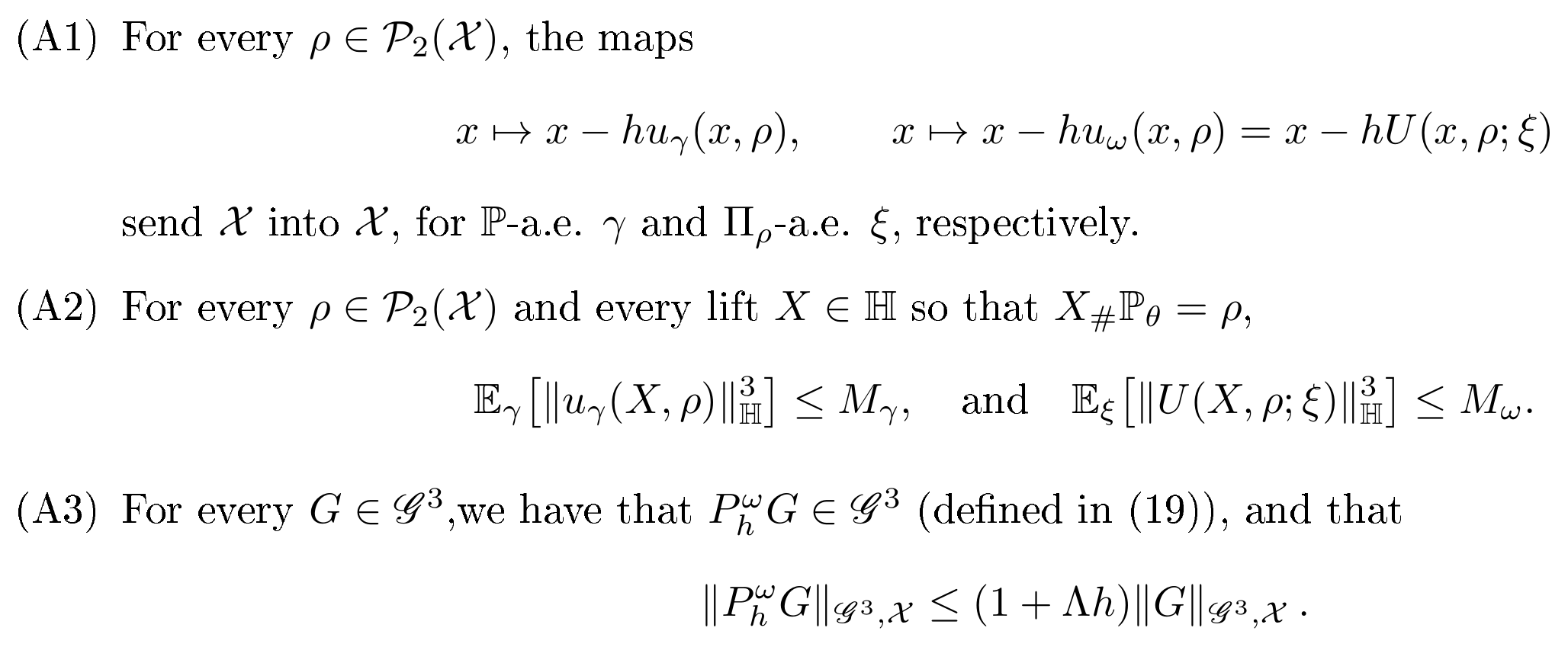
########## {caption="Assumption 6"}

There exist constants

$ h_0>0,\qquad M_\gamma<\infty,\qquad M_\omega<\infty, \qquad \Lambda<\infty $

such that the following conditions hold for all $0<h\le h_0$.

::: {.visual-block data-block-equations="3" data-tables="0" data-figures="0"}

:::

########## {caption="Remark"}

A sufficient condition for Assumption 6(A2) regarding $M_\omega$ is

$ \sup_{\rho\in \mathcal{P}2(\mathcal{X})} \int{\mathcal{X}} |\bar{u}\rho(x)|^3,d\rho(x) <\infty,\quad \text{and}\quad \sup{\rho\in \mathcal{P}2(\mathcal{X})} \int{\mathcal{X}} \big(\operatorname{tr}K_\rho(x,x)\big)^{3/2},d\rho(x) <\infty . $

########## {caption="Remark"}

The following additional conditions on the realizations of the Gaussian field $u_\omega(\cdot, \rho) = U(\cdot, \rho;\xi)$ are sufficient to guarantee that Assumption 6(A3) is satisfied.

1. (Differentiablility in the first argument) For almost all $\omega$, and for all fixed $\rho \in \mathcal{P}(\mathcal{X})$, the function $x \to u_\omega(x, \rho): \mathcal{X} \to \mathcal{X}$ is three times continuously differentiable, with derivatives denoted by $\partial_x^iu_\omega(x, \rho)$.
2. (Lions differentiability in the second argument) For almost all $\omega$, and for all fixed $x \in \mathcal{X}$, the function $\rho \to u_\omega(x, \rho):\mathcal{P}(\mathcal{X}) \to \mathcal{X}$ is three times differentiable in the Lions sense (see Definition 1) with continuous derivatives (in the weak$^*$ topology) denoted by $\partial_\rho u_\omega(x, \rho)$.
3. (Continuity and boundedness) All mixed derivatives $\partial^i_x\partial^j_\rho u_\omega(x, \rho): \mathbb{H}^j \times \mathcal{X}^i \to \mathcal{X}$, $i + j \le 3$ are jointly continuous in $x$ and $\rho$, and are bounded in operator norm. Denote the upper bounds by:

$ \begin{cases} \sup_{\rho \in \mathcal{P}(\mathcal{X}), x \in \mathcal{X}} \Big(| \partial_x u_\omega|\mathrm{op} + |\partial\rho u_\omega|\mathrm{op} \Big)\le C_1\ \sup{\rho \in \mathcal{P}(\mathcal{X}), x \in \mathcal{X}}\Big(| \partial^2_x u_\omega|\mathrm{op} + 2|\partial_x\partial\rho u_\omega |\mathrm{op} + | \partial^2\rho u_\omega|\mathrm{op} \Big) \le C_2 \ \sup{\rho \in \mathcal{P}(\mathcal{X}), x \in \mathcal{X}}\Big(| \partial^3_x u_\omega|\mathrm{op} + 3| \partial^2_x\partial\rho u_\omega|\mathrm{op} + 3 | \partial_x\partial^2\rho u_\omega|\mathrm{op} + |\partial^3\rho u_\omega |_\mathrm{op} \Big)\le C_3 \end{cases} $

Under these additional assumptions, the growth constant $\Lambda$ is upper bounded by:

$ \Lambda \leq 2C_1 + 3C_1C_2 + 3C_2 + C_1^2 + C_3 , \quad \text{ for } h \le 1. $

########## {caption="Theorem 7: Main result"}

Let Assumption 6 hold. Fix a terminal time $T>0$, let $0<h$ be the step-size, and set $n=\lfloor T/h\rfloor$ to be the iteration number. Then, for every terminal observable $G\in\mathscr G^3$ and every initial measure $\rho_0\in \mathcal{P}_2(\mathcal{X})$,

$ \left| \mathbb{E}_\omega \big[ G(\rho_n^X(\rho_0,0)) \big]

\mathbb{E}_\gamma \big[ G(\rho_n^Z(\rho_0,0)) \big] \right| \le C_T h^2,, $

where $\rho_n^X$ and $\rho_n^Z$ are generated by following Equation 12 and 13 starting from the common initial $\rho_0$. The constant is independent of $h$ and $n$ and takes on a specific form:

$ C_T =\frac{T}{6} (M_\omega+M_\gamma) e^{\Lambda T} |G|_{\mathscr G^3, \mathcal{X}},. $

Despite the new geometry and the highly technical use of Lions lifting and differentiability, the result is very intuitive. The matching of the two velocity fields is secured at the level of the mean and the covariance, suggesting the leading-order error should be of order $h^2$. Furthermore, the procedure does not distinguish dissipative or contracting dynamics, so exponential growth in time is also expected. However, gradient flow naturally descends along gradients, so the system is expected to contract, and one may potentially turn the exponential growth into decay. This has not been pursued in this paper.

3.2 Proof of the main result

Proof of Theorem 7: By Assumption 6(A3),

$ | \mathcal{V}k|{\mathscr G^3, \mathcal{X}} \le (1+\Lambda h)^{n-k}|G|{\mathscr G^3, \mathcal{X}} \le e^{\Lambda T}|G|{\mathscr G^3, \mathcal{X}}, \qquad 0\le k\le n. $

Set $G_T:=e^{\Lambda T}|G|_{\mathscr G^3, \mathcal{X}}$. Thus, $| \mathcal{V}k|{\mathscr G^3, \mathcal{X}}\le G_T$, for $0\le k\le n$.

Note that, according to 21, $\mathbb{E}_\omega \bigl[ G(\rho_n^X(\rho_0,0)) \bigr]= \mathcal{V}_0(\rho_0)$, so by telescoping:

$ \begin{aligned}&\mathbb{E}\omega\bigl[ G(\rho_n^X(\rho_0,0)) \bigr] - \mathbb{E}\gamma \bigl[G(\rho_n^Z(\rho_0,0))\bigr]\&\qquad= \mathcal{V}0(\rho_0) - \mathbb{E}\gamma \bigl[\mathcal{V}n(\rho_n^Z) \bigr]\&\qquad=\sum{k=1}^n\mathbb{E}{\gamma{<k}} \left[\mathcal{V}{k-1}(\rho{k-1}^Z) -\mathbb{E}{\gamma_k}\bigl[\mathcal{V}k(\rho_k^Z),\big|,\rho{k-1}^Z\bigr]\right]\&\qquad=\sum{k=1}^n \mathbb{E}{\gamma{<k}} \left[ (P_h^\omega \mathcal{V}k)(\rho{k-1}^Z) - (P_h^\gamma \mathcal{V}k)(\rho{k-1}^Z) \right],\end{aligned} $

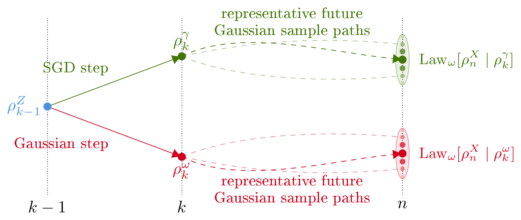
where we used the definition of $\mathcal{V}_k$ to replace the first term and $P_h^\gamma$ in Equation 18 to replace the second term. Figure 1 illustrates the two one-step updates appearing in one summand of Equation 22. The future dashed paths should be read as representative Gaussian sample paths inside the expectation defining $\mathcal{V}_k$.

Equation 18 nicely translates the total trajectory disparity into many one-step error estimates. We now need to show every single term in the summation in the last row of Equation 22 is small. Fix $k\in{1,\ldots,n}$ and fix $\rho\in \mathcal{P}_2(\mathcal{X})$. Let $X\in \mathbb{H}$ be a lift of $\rho$. Let $\widetilde{\mathcal{V}}_k$ denote a law-invariant lift of $\mathcal{V}_k$. Then:

$ (P_h^\omega \mathcal{V}_k)(\rho)

\mathbb{E}_\omega \left[ \widetilde{\mathcal{V}}k(X-hu\omega(X,\rho)) \right],,\quad (P_h^\gamma \mathcal{V}_k)(\rho)

\mathbb{E}_\gamma \left[ \widetilde{\mathcal{V}}k(X-hu\gamma(X,\rho)) \right],. $

Using the Taylor expansion derived in the Lions sense from Theorem 3,

$ \widetilde{\mathcal{V}}_k(X-hH)

\widetilde{\mathcal{V}}_k(X)

h,d_X\widetilde{\mathcal{V}}_k[H] + \frac{h^2}{2},d_X^2\widetilde{\mathcal{V}}_k[H,H] + R_k(X,H), $

where

$ R_k(X,H)

\int_0^1 \frac{(1-\tau)^2}{2} d^3_{X-\tau hH}\widetilde{\mathcal{V}}_k[-hH,-hH,-hH],d\tau . $

Therefore

$ (P_h^\omega \mathcal{V}_k)(\rho)

(P_h^\gamma \mathcal{V}_k)(\rho)

\mathrm{I}_k(\rho)+\mathrm{II}_k(\rho)+\mathrm{III}_k(\rho), $

where the three terms are:

• Leading order disparity:

$ \mathrm{I}_k(\rho)

-h,d_X\widetilde{\mathcal{V}}k \left[ \mathbb{E}\omega u_\omega(X,\rho)-\mathbb{E}\gamma u\gamma(X,\rho) \right]=0,, $

according to Assumption 6(A3), $\mathbb{E}\omega H\omega = \mathbb{E}\gamma H\gamma = \bar{u}_\rho\circ X$.

• Second order disparity:

$ \mathrm{II}k(\rho)= \frac{h^2}{2}\left(\mathbb{E}\omega \left[ d_X^2\widetilde{\mathcal{V}}k[u\omega,u_\omega]\right] -\mathbb{E}\gamma \left[ d_X^2\widetilde{\mathcal{V}}k[u\gamma,u\gamma]\right] \right)=0,, $

and this comes from Assumption 6(A3) and the application of Proposition 4 on bilinear operator.

• Third order disparity is:

$ \mathrm{III}_k(\rho)

\mathbb{E}\omega R_k(X,u\omega)

\mathbb{E}\gamma R_k(X,u\gamma). $

By Assumption 6(A1), the points $X-hH_\omega$ and $X-hH_\gamma$ belong to $\mathbb{H}$ almost surely. Since $\mathcal{X}$ is convex, the whole segments $X-\tau hu_\omega$ and $X-\tau hu_\gamma$ are in $\mathbb{H}$ for all $0\le\tau\le1$. Hence

$ \max\left{|d^3_{X-\tau hu_\omega}\widetilde{\mathcal{V}}k|{\mathrm{op}},,|d^3_{X-\tau hu_\gamma}\widetilde{\mathcal{V}}k|{\mathrm{op}}\right} \le | \mathcal{V}k|{\mathscr G^3, \mathcal{X}}\le G_T, $

and similarly for $H_\gamma$.

Putting these all together, and use Assumption 6(A2), we obtain, for every $\rho\in \mathcal{P}_2(\mathcal{X})$,

$ \left| (P_h^\omega \mathcal{V}_k)(\rho)

(P_h^\gamma \mathcal{V}k)(\rho) \right| \le \frac{h^3}{6} G_T (M\omega+M_\gamma). $

Combining Equation 22 and 23, we get

$ \begin{aligned} & \left| \mathbb{E}_\omega \bigl[ G(\rho_n^X(\rho_0,0)) \bigr]

\mathbb{E}\gamma \bigl[ G(\rho_n^Z(\rho_0,0)) \bigr] \right| \ &\qquad \le \sum{k=1}^n \mathbb{E}{\gamma{<k}} \left[ \left| (P_h^\omega \mathcal{V}k)(\rho{k-1}^Z)

(P_h^\gamma \mathcal{V}k)(\rho{k-1}^Z) \right| \right] \ &\qquad \le n,\frac{h^3}{6}G_T(M_\omega+M_\gamma). \end{aligned} $

Since $nh\le T$, this gives

$ \left| \mathbb{E}_\omega \bigl[ G(\rho_n^X(\rho_0,0)) \bigr]

\mathbb{E}\gamma \bigl[ G(\rho_n^Z(\rho_0,0)) \bigr] \right| \le \frac{T}{6} (M\omega+M_\gamma) e^{\Lambda T} |G|_{\mathscr G^3, \mathcal{X}} h^2. $

This proves the theorem.

4. Numerical experiments

Section Summary: The section outlines two numerical experiments that test a stochastic iteration scheme and its moment-matched Gaussian approximation. The first uses an exactly solvable quadratic benchmark driven by skewed two-point noise to isolate and confirm a second-order weak error that scales as C h² plus higher-order terms, verified by both closed-form expectations and large-scale Monte Carlo runs. The second examines a stochastic inverse problem of recovering a distribution from randomly sampled first- and second-moment targets, with state-dependent velocities represented via a rank-one Gaussian field and propagated exactly through affine maps on an interval.

We present two complementary experiments for the stochastic iteration Equation 12 and its moment-matched Gaussian approximation Equation 13. The first is an exactly solvable benchmark that isolates the second-order weak error. The second is a stochastic inverse problem in which a probability distribution is reconstructed from randomly sampled moment measurements; in this case the velocity and its covariance depend on the current measure.

For a terminal observable $\mathcal G$ and $n=T/h$, we report

$ e_h(\mathcal G,T) :=\left| \mathbb{E}\gamma[\mathcal G(\rho_n^Z)] -\mathbb{E}\omega[\mathcal G(\rho_n^X)] \right|. $

All computations use a Euclidean projection $\pi_{\mathcal X}$ after each explicit update as a compact-domain safeguard. Projection activations are recorded in every Monte Carlo experiment; none occurred in the results below.

4.1 Solvable quadratic benchmark

Let $\mathcal X=[-10,10]$ and consider

$ \mathcal E_\gamma(\rho) :=\frac12\int_{\mathcal X}(x-\gamma)^2,d\rho(x), \qquad u_\gamma(x,\rho)=x-\gamma. $

We use the skew two-point distribution

$ \mathbb{P}(\gamma=2)=\frac13, \qquad \mathbb{P}(\gamma=-1)=\frac23. $

It satisfies $\mathbb{E}\left[\gamma\right]=0$, $\mathbb{E}\left[\gamma^2\right]=2$, and $\mathbb{E}\left[\gamma^3\right]=2$. The moment-matched Gaussian parameter is therefore $\omega\sim\mathcal N(0,2)$, with velocity $u_\omega(x,\rho)=x-\omega$.

Writing

$ \pi_{\mathcal X}(x):=\min{10,\max{-10,x}}, $

the implemented recursions are

$ \begin{aligned}\rho_{k+1}^Z &=\bigl(\pi_{\mathcal X}\circ((1-h)\operatorname{Id}+h\gamma_k)\bigr)# \rho_k^Z,\\rho{k+1}^X &=\bigl(\pi_{\mathcal X}\circ((1-h)\operatorname{Id}+h\omega_k)\bigr)_# \rho_k^X.\end{aligned} $

We initialize at $\rho_0=\delta_0$ and take

$ \mathcal G(\rho):=\int_{\mathcal X}\sin(x),d\rho(x). $

For $0<h\leq1$, the original process never reaches the boundary because each update is a convex combination of the current state and $\gamma_k\in{-1,2}$. Consequently,

$ x_n^Z=h\sum_{j=1}^n(1-h)^{n-j}\gamma_j, \qquad \rho_n^Z=\delta_{x_n^Z}, $

and independence gives

$ \mathbb{E}\gamma[\mathcal G(\rho_n^Z)] =\operatorname{Im} \prod{r=0}^{n-1} \left( \frac13e^{2ih(1-h)^r} +\frac23e^{-ih(1-h)^r} \right). $

The projected Gaussian recursion is symmetric about zero, so $\mathbb{E}_\omega[\mathcal G(\rho_n^X)]=0$. A cumulant expansion of Equation 29, with $T=nh$ fixed, yields

$ e_h(\mathcal G,T) =C_h^2+\mathcal O(h^3), \qquad C_:=\frac{1-e^{-3T}}9. $

The nonzero coefficient is generated by the third-moment mismatch between the skew two-point noise and its Gaussian surrogate.

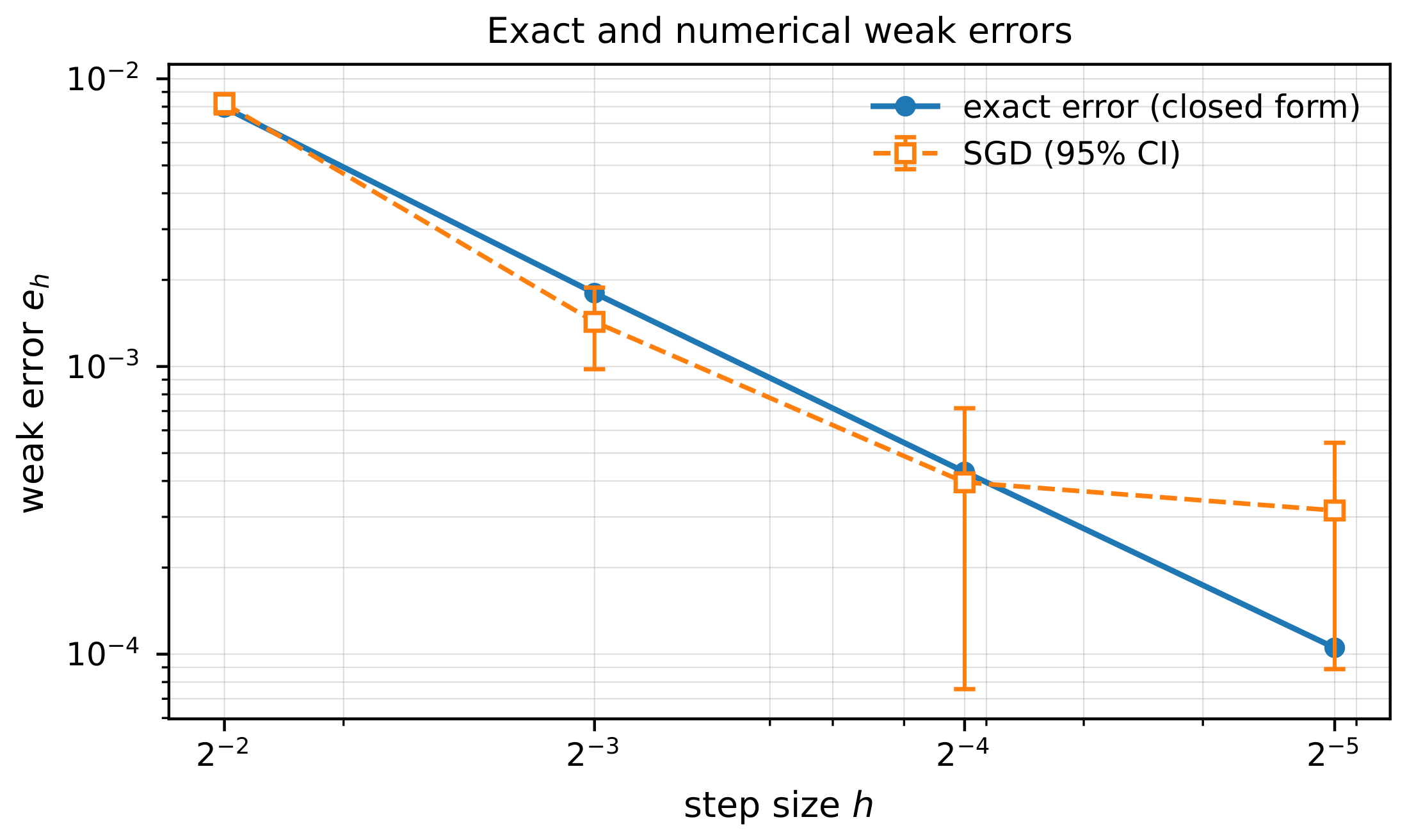
Figure 2 directly compares the exact weak error at $T=1$ with numerical estimates obtained from simulated trajectories for $h=2^{-\ell}$, $\ell=2,\ldots,5$. At each reported step size, we simulate $10^6$ trajectories of each dynamics, organized into $5\times10^5$ independent pairs. The error bars are $95%$ confidence intervals for the absolute weak error, and the exact value lies inside the interval at every reported resolution. No projection $\pi_{\mathcal X}$ was activated.

This benchmark demosntrates the result in Theorem 7. Matching the mean and covariance removes the first- and second-order contributions in the one-step Taylor expansion, while the third-moment mismatch produces a local error of order $h^3$; over $n=T/h$ steps this accumulates to the global order $h^2$ predicted by the theorem. Because $C_*\neq0$, the exact expansion Equation 30 also shows that the second-order bound is sharp in general.

{width=80%}

4.2 Random-moment distribution reconstruction

We next study an optimization problem that is to reconstruct a distribution that matches desired first two moments:

$ \mathcal{E}(\rho) =\frac{p}{2}(m_\rho-y_1)^2 +\frac{1-p}{2}(q_\rho-y_2)^2 = \mathbb{E}{\gamma \sim \text{Bernouli}(p)} [\mathcal{E}{\gamma + 1}(\rho)], $

where $\gamma \in {0, 1}$ is a Bernouli random variable with parameter $p$, and

$ \mathcal E_1(\rho):=\frac12(m_\rho-y_1)^2, \qquad \mathcal E_2(\rho):=\frac12(q_\rho-y_2)^2,. $

Here $m_\rho$ and $q_\rho$ are the first two moments:

$ m_\rho:=\int_{\mathcal X}x,d\rho(x), \qquad q_\rho:=\int_{\mathcal X}x^2,d\rho(x),. $

Numerically we set the targets $y_1=0.75$ and $y_2=1$ and $p=1/3$. Conditioned on $\rho$, one can compute the mean function and covariance kernel:

$ \begin{aligned}\bar{u}\rho(x) &=pu_1(x,\rho)+(1-p)u_2(x,\rho),\K\rho(x,y) &=p(1-p) \bigl(u_1(x,\rho)-u_2(x,\rho)\bigr) \bigl(u_1(y,\rho)-u_2(y,\rho)\bigr),\end{aligned} $

where the two velocities are

$ u_1(x,\rho)=m_\rho-y_1, \qquad u_2(x,\rho)=2(q_\rho-y_2)x. $

Since the covariance matrix is rank one, the matching Gaussian field is represented by a single Gaussian variable:

$ U(x,\rho;\xi) =\bar{u}_\rho(x) +\sqrt{p(1-p)} \bigl(u_1(x,\rho)-u_2(x,\rho)\bigr)\xi, \qquad \xi\sim\mathcal N(0,1),. $

We take $\mathcal X=[-20,20]$ and $\rho_0=\operatorname{Unif}[-1,1]$. The projection $\pi_{\mathcal X}$ is applied after each update. Both velocities in Equation 34 are affine in $x$; as long as the boundary is inactive, each realization is therefore an affine image of the initial uniform distribution. We propagate this affine representation and evaluate its moments analytically. The terminal observable is

$ \mathcal G(\rho):=m_\rho^3. $

This cubic statistic is smooth and is sensitive to the first unmatched moment. For each step size $h$, we estimate the difference between two dynamics with $2\times10^6$ coupled paths.

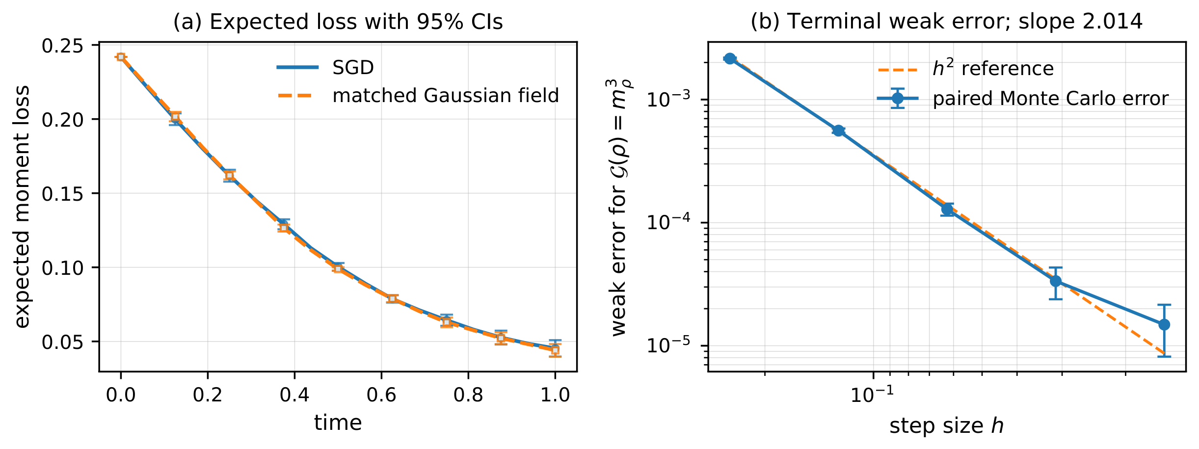
The results are presented in Figure 3. The left panel of Figure 3 shows $\mathbb{E}[\mathcal E(\rho_t)]$ for $h=2^{-4}$, estimated from $25$ independently sampled trajectories for each dynamics. Pointwise $95%$ Student-$t$ confidence intervals are shown at nine equally spaced times. The right panel reports the terminal weak error at $T=1$ for $h=2^{-\ell}$, $\ell=2,\ldots,6$, using $2\times10^6$ paths per step size. A log-log fit over the four points with signal-to-noise ratio greater than five gives order $2.014$. The smallest-step result is shown with its $95%$ confidence interval but is excluded from the fit because the Monte Carlo error dominates. No projection activation occurred in any of the reported trajectories.

This example tests the same conclusion in the state-dependent setting for which the analysis was developed. Equations 33 and 35 match the conditional mean and covariance of the velocity field at every current measure. The smooth cubic observable Equation 36 detects the remaining higher-moment discrepancy, and the fitted order $2.014$ is consistent with the $\mathcal O(h^2)$ estimate of Theorem 7. The overlapping objective curves further indicate that the Gaussian approximation dynamics reproduces the stochastic gradient dynamics.

5. Conclusion

Section Summary: The paper establishes a second-order weak approximation to stochastic Wasserstein gradient flows by replacing the true velocity with a state-dependent Gaussian field that matches its conditional mean and covariance. This matching, combined with a Taylor expansion argument and stability of the resulting transitions, produces a global error of order h squared for smooth test functions after any fixed time horizon. Numerical tests on quadratic and moment-reconstruction problems confirm that the predicted rate is sharp, while several open questions remain about relaxing the compactness and moment assumptions and about passing to a continuous-time stochastic PDE limit.

We have established a second-order weak approximation of stochastic Wasserstein gradient iterations by a discrete-time scheme driven by a state-dependent Gaussian velocity field. A Gaussian field that matches the conditional mean and covariance of the original stochastic velocity is capable of capturing the stochastic Wasserstein gradient dynamics with weak error of $h^2$ for sufficiently regular terminal observables, as discovered by Theorem 7.

The proof also identifies the mechanism behind this rate. A third-order Taylor expansion in the Lions sense reduces the one-step comparison to the first moments, covariance terms, and a cubic remainder. Moment matching makes the first- and second-order contributions agree, leaving a local discrepancy of order $h^3$. The telescoping weak-error representation and the stability of the Gaussian transition operators then accumulate these local errors over $T/h$ steps to produce the global second-order estimate. Thus, the Gaussian approximation retains precisely the fluctuation information needed at the order considered here.

The numerical experiments support and complement this analysis. In the solvable quadratic benchmark, the exact nonzero $h^2$ coefficient shows that the theoretical order is sharp in general. The random-moment reconstruction problem demonstrates the same behavior when both the velocity and its covariance depend on the evolving measure. In both cases, the compact-domain projection remained inactive, and the measured rates therefore reflect the interior moment-matching mechanism analyzed in the paper.

Several questions remain open. The present result relies on a compact-domain invariance condition, uniform third-moment bounds, and regularity propagation for the Gaussian transition operators. It would be useful to replace these assumptions with verifiable conditions for broader classes of energies, to treat unbounded domains and regimes in which a boundary mechanism is active, and to study the continuous-time stochastic Wasserstein dynamics suggested by the Gaussian approximation. Another direction is to investigate whether matching additional moments can yield higher-order weak schemes. These extensions would further clarify the role of Gaussian surrogates in stochastic optimization over probability measures. Lastly, we compare on the discrete-in-time level. Drawing inspiration from [9], it is possible to pass the $h\to0$ limit to devise a modified stochastic differential PDE. However, this will necessarily trigger the study of the well-posedness of SPDEs over $\mathcal P_2(\mathcal X)$ when the velocity field is a Gaussian field that nonlinearly depends on the probability state. It is not yet evident.

References

Section Summary: This section compiles a list of academic citations drawn from mathematics, probability theory, and machine learning research. The references span foundational papers on stochastic approximation and optimization methods dating back to the 1950s, as well as more recent studies on diffusion processes, gradient flows, optimal transport, and mean-field models. Together they point to theoretical tools commonly used to analyze algorithms for large-scale computation and global minimization problems.

[1] Robbins, Herbert and Monro, Sutton (1951). A stochastic approximation method. The Annals of Mathematical Statistics. pp. 400–407.

[2] Bottou et al. (2018). Optimization methods for large-scale machine learning. SIAM Review. 60(2). pp. 223–311.

[3] Geman, Stuart and Hwang, Chii-Ruey (1986). Diffusions for global optimization. SIAM Journal on Control and Optimization. 24(5). pp. 1031–1043.

[4] Chiang et al. (1987). Diffusion for global optimization in $\mathbb R^n$. SIAM Journal on Control and Optimization. 25(3). pp. 737–753.

[5] Kushner, Harold J (1987). Asymptotic global behavior for stochastic approximation and diffusions with slowly decreasing noise effects: global minimization via Monte Carlo. SIAM Journal on Applied Mathematics. 47(1). pp. 169–185.

[6] Hwang, Chii-Ruey and Sheu, Shuenn-Jyi (1990). Large-time behavior of perturbed diffusion Markov processes with applications to the second eigenvalue problem for Fokker–Planck operators and simulated annealing. Acta Applicandae Mathematica. 19(3). pp. 253–295.

[7] Gelfand, Saul B and Mitter, Sanjoy K (1991). Recursive stochastic algorithms for global optimization in $\mathbb R^d$. SIAM Journal on Control and Optimization. 29(5). pp. 999–1018.

[8] Cheng et al. (2020). Stochastic gradient and Langevin processes. In International Conference on Machine Learning. pp. 1810–1819.

[9] Li et al. (2019). Stochastic Modified Equations and Dynamics of Stochastic Gradient Algorithms I: Mathematical Foundations. Journal of Machine Learning Research. 20(40). pp. 1–47.

[10] Jordan et al. (1998). The variational formulation of the Fokker–Planck equation. SIAM Journal on Mathematical Analysis. 29(1). pp. 1–17.

[11] Liu, Qiang and Wang, Dilin (2016). Stein Variational Gradient Descent: A General Purpose Bayesian Inference Algorithm. In Advances in Neural Information Processing Systems. pp. 2378–2386. https://neurips.cc.

[12] Xie, Yao and Cheng, Xiuyuan (2025). Flow-Based Generative Models as Iterative Algorithms in Probability Space: An Intuitive Mathematical Framework [Special Issue on the Mathematics of Deep Learning]. IEEE Signal Processing Magazine. 43(2). pp. 37–50. doi:10.1109/MSP.2025.3609527.

[13] Han et al. (2026). One-step generative modeling via Wasserstein gradient flows. arXiv preprint arXiv:2605.11755.

[14] Zhiyan Ding et al. (2022). Overparameterization of Deep ResNet: Zero Loss and Mean-field Analysis. Journal of Machine Learning Research. 23(48). pp. 1–65. http://jmlr.org.

[15] Rotskoff, Grant and Vanden-Eijnden, Eric (2018). Parameters as interacting particles: long time convergence and asymptotic error scaling of neural networks. In Advances in Neural Information Processing Systems. https://proceedings.neurips.cc/paper_files/paper/2018/file/196f5641aa9dc87067da4ff90fd81e7b-Paper.pdf.

[16] Chizat, Lénaïc and Bach, Francis (2018). On the Global Convergence of Gradient Descent for Over-parameterized Models using Optimal Transport. In Advances in Neural Information Processing Systems (NeurIPS). pp. 3036–3046. https://neurips.cc.

[17] Geshkovski et al. (2025). A mathematical perspective on Transformers. Bulletin of the American Mathematical Society. 62(3). pp. 427–479. doi:10.1090/bull/1832.

[18] Ambrosio et al. (2005). Gradient Flows: in Metric Spaces and in the Space of Probability Measures. Birkhäuser Verlag.

[19] Cédric Villani (2003). Topics in Optimal Transportation. American Mathematical Society.

[20] Nurbekyan et al. (2023). Efficient natural gradient descent methods for large-scale PDE-based optimization problems. SIAM Journal on Scientific Computing. 45(4). pp. A1621–A1655.

[21] Wilfrid Gangbo and Adrian Tudorascu (2019). On Differentiability in the Wasserstein Space and Well-Posedness for Hamilton–Jacobi Equations. Journal de Mathématiques Pures et Appliquées. 125. pp. 119–174.

[22] René Carmona and François Delarue (2018). Probabilistic Theory of Mean Field Games with Applications I: Mean Field FBSDEs, Control, and Games. Springer.

[23] Pierre Cardaliaguet (2013). Notes on Mean Field Games (from P.-L. Lions' Lectures at Collège de France). Unpublished lecture notes.

[24] Filippo Santambrogio (2015). Optimal Transport for Applied Mathematicians. Birkhäuser.

[25] Wanner, Mathias and Mezić, Igor (2022). Robust approximation of the stochastic Koopman operator. SIAM Journal on Applied Dynamical Systems. 21(3). pp. 1930–1951.