A Model of Inductive Bias Learning

Jonathan Baxter

article2000JAIR1,340 citations

Establishes a foundational theoretical framework for automatically learning inductive biases across related tasks, proving explicit generalization bounds that demonstrate how multi-task experience drastically reduces the sample complexity required to learn novel problems.

Listen

The performance of machine learning algorithms heavily depends on choosing an appropriate hypothesis space or inductive bias. When this choice is too broad, the system requires an impractical amount of data to generalize effectively; when it is too narrow, it cannot find an accurate solution. Historically, practitioners have relied on manual, expert-driven heuristics to select these inductive biases, a process that is often costly, error-prone, and difficult to scale across complex domains.

The article develops and analyzes a formal mathematical framework for automatically learning inductive bias across an environment of related learning tasks. Its primary objective is to prove theoretical guarantees on sample complexity, evaluating how many tasks and how many examples per task are required for a learner to discover a restricted representation that reliably transfers to novel, unseen problems.

To establish these guarantees, the author generalizes classical single-task learning theory using an empirical process approach. The framework models learning problems as probability distributions drawn from an overarching environment distribution. The analysis evaluates uniform convergence across families of hypothesis spaces using metric covering numbers and capacity dimensions, deriving explicit upper and lower bounds for both general task settings and specific neural network feature-learning models.

The article yields three core findings. First, learning across multiple related tasks dramatically reduces the data required per individual task; as the number of observed tasks increases, the number of training examples needed per task decreases toward the theoretical minimum needed when the true representation is known. Second, a learner that finds a shared representation performing well on a sufficiently large set of training tasks will, with high probability, generalize effectively to future, unseen tasks drawn from the same environment. Third, when applied to neural networks, the required number of training tasks scales with the complexity of the feature representation, while the examples needed per task scale with the sum of the output parameters and the feature parameters divided by the number of tasks, a bound proved to be essentially tight for threshold networks.

These findings demonstrate that multi-task bias learning converts high-complexity representation learning into a manageable problem by amortizing the data collection burden across many tasks. For organizational leaders and practitioners, this means systems designed to handle streams of related challenges—such as face recognition, speech analysis, or multi-disease diagnostics—can achieve high accuracy on new tasks with minimal data and lower operational costs once the underlying feature representation is learned.

Organizations developing machine learning pipelines for related problem domains should transition from training isolated single-task models to joint multi-task representation learning architectures. Where practical, teams should implement shared feature maps trained across existing operational tasks before deploying lightweight adapters for novel use cases. However, researchers and practitioners must still develop robust methods for assessing whether a given set of tasks is genuinely related before pooling data.

The primary theoretical limitation is that the model assumes candidate tasks are independently sampled from a stationary environment distribution, which may not hold in non-stationary operational settings. Furthermore, while the derived upper bounds on the required number of tasks scale with feature complexity, empirical evidence suggests these bounds can be pessimistic in practice. Confidence in the mathematical convergence guarantees is high, but practitioners should exercise caution when grouping tasks whose relatedness cannot be empirically or domain-verified.

Australian National University hierarchical model online learning training sample inductive bias learning computational learning theory hierarchical Bayes

arXiv: 1106.0245

Paper: Multitask Learning, RICH CARUANA (1997). Caruana’s seminal work empirically establishes multitask learning and shared representations across related tasks, providing the foundational conceptual paradigm formalized theoretically by Baxter.

Paper: Regularized multi--task learning, T. Evgeniou et al. (2004). Develops a regularized kernel and SVM framework that operationalizes Baxter's bias-learning principles into convex multi-task learning formulations.
Paper: Convex multi-task feature learning, Andreas Argyriou et al. (2008). Extends the theoretical goal of learning a shared hypothesis space into a rigorous convex optimization framework for multi-task feature representation learning.
Paper: Multi-task Gaussian Process Prediction, Edwin V. Bonilla et al. (2007). Applies inductive bias sharing across related tasks within a non-parametric Bayesian framework using multi-task Gaussian processes.
Paper: A Survey on Multi-Task Learning, Yu Zhang et al. (2017). Provides a comprehensive survey classifying multi-task learning architectures and theoretical bounds that build upon Baxter's environment-of-tasks model.
Paper: An Overview of Multi-Task Learning in Deep Neural Networks, Sebastian Ruder (2017). Surveys how the theoretical mechanisms of shared inductive bias and multi-task representation learning are realized in modern deep neural networks.
Paper: A Survey on Transfer Learning, Sinno Jialin Pan et al. (2010). Surveys the broader paradigm of transfer learning and domain adaptation that emerged from theoretical multi-task bias-learning formulations.
Paper: A theory of learning from different domains, Shai Ben-David et al. (2010). Formalizes distribution shift and cross-domain generalization bounds, generalizing the learning-to-learn and environment-based guarantees to transfer learning.
Paper: Meta-Learning with Latent Embedding Optimization, Andrei A. Rusu et al. (2018). Extends task-environment learning to gradient-based meta-learning by learning low-dimensional latent task embeddings for rapid adaptation.

Cover for A Model of Inductive Bias Learning

Abstract

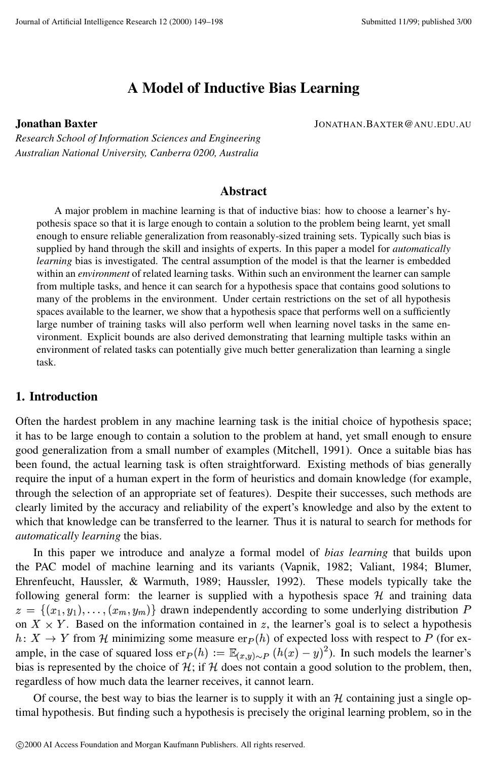
A major problem in machine learning is that of inductive bias: how to choose a learner's hypothesis space so that it is large enough to contain a solution to the problem being learnt, yet small enough to ensure reliable generalization from reasonably-sized training sets. Typically such bias is supplied by hand through the skill and insights of experts. In this paper a model for automatically learning bias is investigated. The central assumption of the model is that the learner is embedded within an environment of related learning tasks. Within such an environment the learner can sample from multiple tasks, and hence it can search for a hypothesis space that contains good solutions to many of the problems in the environment. Under certain restrictions on the set of all hypothesis spaces available to the learner, we show that a hypothesis space that performs well on a sufficiently large number of training tasks will also perform well when learning novel tasks in the same environment. Explicit bounds are also derived demonstrating that learning multiple tasks within an environment of related tasks can potentially give much better generalization than learning a single task.

Topics

hierarchical model online learning training sample

Keywords

inductive bias learning computational learning theory hierarchical Bayes feature learning internal representations generalization performance threshold networks gradient descent inductive logic

1. Introduction
1.1 Related Work
1.2 Overview of the Paper
2. The Bias Learning Model
2.1 Single-Task Learning
2.2 The Bias Learning Model
2.3 Covering Numbers
2.4 Uniform Convergence for Bias Learners
2.5 Choosing the Hypothesis Space Family
2.6 Learning Multiple Tasks
3. Feature Learning
3.1 The Feature Learning Model
3.3 Learning Neural Network Features
3.3.1 Multiple Output Classes
3.3.2 Sample Complexity Bounds for Neural-Network Feature Learning
3.3.3 Discussion
3.3.4 Comparison with Traditional Multiple-Class Classification
3.4 Learning Multiple Tasks with Boolean Feature Maps
3.4.1 Upper and Lower Bounds for Learning Tasks with Boolean Hypothesis Space Families
4. Conclusion
Acknowledgements
Appendix A. Uniform Convergence Results
A.1 Proof of Theorem 18
A.1.2 Second Symmetrization
A.2 Proof of Theorem 2
B.1 Bounding
B.3 Proof of Theorem 7
Appendix C. Proof of Theorem 14
References

Knowls

Knowl 1 — Formal Framework of Inductive Bias Learning
definition
In the formal model of inductive bias learning (or learning-to-learn), the learning problem is formulated across an environment of tasks rather than a single fixed task:
- Input and Output Spaces: An input space $X$ and output space $Y$ , both assumed to be separable metric spaces.
- Loss Function: A bounded loss function $l: Y imes Y \to [0, 1]$ .
- Task and Environment: A learning task is represented by a probability distribution $P$ on $X \times Y$ . Let $\mathcal{P}$ denote the set of all probability distributions on $X \times Y$ . An environment is represented by a pair $(\mathcal{P}, Q)$ , where $Q$ is an environmental probability distribution on $\mathcal{P}$ governing the generation of tasks.
- Hypothesis Space Family: A set $\mathbb{H} = \{H\}$ where each element $H \in \mathbb{H}$ is a hypothesis space of candidate functions $h: X \to Y$ . Choosing a hypothesis space $H \in \mathbb{H}$ represents choosing an inductive bias.
- Environmental Loss: The true error of a hypothesis $h$ on task $P$ is $\mathrm{er}_P(h) := \mathbb{E}_{(x,y)\sim P}[l(h(x), y)]$ . The environmental loss of a hypothesis space $H \in \mathbb{H}$ across the environment $(\mathcal{P}, Q)$ is defined as:
$\mathrm{er}_Q(H) := \int_{\mathcal{P}} \inf_{h \in H} \mathrm{er}_P(h) dQ(P)$
- Sample and Empirical Loss: The learner receives an $(n, m)$ -sample $\mathbf{z} = (z_1, \dots, z_n)$ , where $n$ tasks $P_1, \dots, P_n$ are drawn i.i.d. according to $Q$ , and for each task $P_i$ , a training set $z_i = \{(x_{i1}, y_{i1}), \dots, (x_{im}, y_{im})\}$ of $m$ examples is sampled i.i.d. from $P_i$ . The empirical loss of $H$ on $\mathbf{z}$ is:
$\widehat{\mathrm{er}}_{\mathbf{z}}(H) := \frac{1}{n} \sum_{i=1}^n \inf_{h \in H} \widehat{\mathrm{er}}_{z_i}(h)$

where $\widehat{\mathrm{er}}_{z_i}(h) := \frac{1}{m} \sum_{j=1}^m l(h(x_{ij}), y_{ij})$ is the empirical error on the $i$ -th task dataset.
Knowl 2 — Uniform Convergence Bounds for Inductive Bias Learning
theoretical result
Let $X$ and $Y$ be separable metric spaces, $l: Y \times Y \to [0, 1]$ a bounded loss function, $(\mathcal{P}, Q)$ an environment of tasks, and $\mathbb{H} = \{H\}$ a permissible family of hypothesis spaces.

Define the task-loss function $H^*(P) := \inf_{h \in H} \mathrm{er}_P(h)$ for each $H \in \mathbb{H}$ , with class $\mathbb{H}^* := \{H^* : H \in \mathbb{H}\}$ . For any distribution $Q$ on $\mathcal{P}$ , let $d_Q(H_1^*, H_2^*) := \int_{\mathcal{P}} |H_1^*(P) - H_2^*(P)| dQ(P)$ , and define capacity $C(\epsilon, \mathbb{H}^*) := \sup_Q \mathcal{N}(\epsilon, \mathbb{H}^*, d_Q)$ .

For any sequence of $n$ hypotheses $(h_1, \dots, h_n)$ from a single $H \in \mathbb{H}$ , define $(h_1, \dots, h_n)_l(x_1, y_1, \dots, x_n, y_n) := \frac{1}{n} \sum_{i=1}^n l(h_i(x_i), y_i)$ , and let $\mathbb{H}_l^n := \bigcup_{H \in \mathbb{H}} \{ (h_1, \dots, h_n)_l : h_1, \dots, h_n \in H \}$ . For product distribution $\mathbf{P} = P_1 \times \dots \times P_n$ on $(X \times Y)^n$ , define the metric $d_{\mathbf{P}}(\mathbf{h}_l, \mathbf{h}'_l) := \int_{(X \times Y)^n} |\mathbf{h}_l - \mathbf{h}'_l| d\mathbf{P}$ , and capacity $C(\epsilon, \mathbb{H}_l^n) := \sup_{\mathbf{P}} \mathcal{N}(\epsilon, \mathbb{H}_l^n, d_{\mathbf{P}})$ .

If the number of sampled tasks $n$ satisfies:

$n \ge \max\left\{ \frac{256}{\epsilon^2} \log \frac{8 C(\epsilon/32, \mathbb{H}^*)}{\delta}, \frac{64}{\epsilon^2} \right\}$

and the number of training examples per task $m$ satisfies:

$m \ge \max\left\{ \frac{256}{n \epsilon^2} \log \frac{8 C(\epsilon/32, \mathbb{H}_l^n)}{\delta}, \frac{64}{\epsilon^2} \right\}$

then with probability at least $1 - \delta$ over the random draw of the $(n, m)$ -sample $\mathbf{z}$ , every hypothesis space $H \in \mathbb{H}$ satisfies:

$\mathrm{er}_Q(H) \le \widehat{\mathrm{er}}_{\mathbf{z}}(H) + \epsilon$
Knowl 3 — Generalization Sample Complexity for Novel Tasks with Learnt Bias
theoretical result
Once a hypothesis space $H \in \mathbb{H}$ has been selected by a bias learner from an environment $(\mathcal{P}, Q)$ such that its empirical error $\widehat{\mathrm{er}}_{\mathbf{z}}(H)$ is small, learning a novel task $P \sim Q$ using the fixed hypothesis space $H$ requires a substantially reduced sample size.

Let $z = \{(x_1, y_1), \dots, (x_m, y_m)\}$ be an i.i.d. sample of size $m$ from a novel task $P$ on $X \times Y$ . Let $H$ be a permissible hypothesis space with loss function class $H_l := \{ (x, y) \mapsto l(h(x), y) : h \in H \}$ , and capacity $C(\epsilon, H_l) := \sup_P \mathcal{N}(\epsilon, H_l, d_P)$ where $d_P(h_l, h'_l) = \int_{X \times Y} |h_l(x,y) - h'_l(x,y)| dP(x,y)$ .

For any $\epsilon, \delta \in (0, 1)$ , if the number of training examples $m$ for the novel task satisfies:

$m \ge \max\left\{ \frac{64}{\epsilon^2} \log \frac{4 C(\epsilon/16, H_l)}{\delta}, \frac{16}{\epsilon^2} \right\}$

then with probability at least $1 - \delta$ over the choice of $z$ , every $h \in H$ satisfies:

$\mathrm{er}_P(h) \le \widehat{\mathrm{er}}_z(h) + \epsilon$

Because $C(\epsilon, H_l)$ depends only on the size of the learned space $H$ rather than the much larger family $\bigcup_{H \in \mathbb{H}} H_l$ , the sample complexity for learning novel tasks is greatly reduced.
Knowl 4 — Capacity Bounds for Composed Feature Hypothesis Space Families
theoretical result
Let feature maps $f \in \mathcal{F}$ map $X \to V$ , and let output function classes $\mathcal{G}$ map $V \to Y$ . For a bounded loss $l: Y \times Y \to [0, 1]$ , define the combined loss class $\mathcal{G}_l$ on $V \times Y$ by $g_l(v, y) := l(g(v), y)$ . Each feature map $f \in \mathcal{F}$ defines a hypothesis space $G \circ f := \{ g \circ f : g \in \mathcal{G} \}$ , yielding the family $\mathbb{H} = \{ G \circ f : f \in \mathcal{F} \}$ .

Define the pseudo-metric on feature maps $\mathcal{F}$ pulled back through $\mathcal{G}_l$ under probability measure $P$ on $X \times Y$ :

$d_{[P, \mathcal{G}_l]}(f, f') := \int_{X \times Y} \sup_{g \in \mathcal{G}_l} |g(f(x), y) - g(f'(x), y)| dP(x, y)$

and the corresponding capacity $C_{\mathcal{G}_l}(\epsilon, \mathcal{F}) := \sup_P \mathcal{N}(\epsilon, \mathcal{F}, d_{[P, \mathcal{G}_l]})$ .

For any $\epsilon, \epsilon_1, \epsilon_2 > 0$ such that $\epsilon = \epsilon_1 + \epsilon_2$ , the capacities of the multi-task loss class $\mathbb{H}_l^n$ and environmental loss class $\mathbb{H}^*$ satisfy:

$C(\epsilon, \mathbb{H}_l^n) \le C(\epsilon_1, \mathcal{G}_l)^n C_{\mathcal{G}_l}(\epsilon_2, \mathcal{F})$

$C(\epsilon, \mathbb{H}^*) \le C_{\mathcal{G}_l}(\epsilon, \mathcal{F})$
Knowl 5 — Sample Complexity for Continuous Neural Network Feature Learning
theoretical result
Consider a neural network hypothesis space family where each hypothesis space $H_w \in \mathbb{H}$ consists of squashed linear output functions composed with a shared neural network feature map $\Phi_w = (\phi_{w, 1}, \dots, \phi_{w, k}): \mathbb{R}^d \to [0, 1]^k$ containing $W$ total adjustable weights $w \in \mathbb{R}^W$ :

$H_w := \left\{ x \mapsto \sigma\left( \sum_{i=1}^k \alpha_i \phi_{w,i}(x) + \alpha_0 \right) : (\alpha_0, \alpha_1, \dots, \alpha_k) \in D' \right\}$

where $D' \subset \mathbb{R}^{k+1}$ is bounded, $\sigma: \mathbb{R} \to [0, 1]$ is Lipschitz continuous, and the loss function $l$ is squared loss on $Y = [0, 1]$ .

The capacities satisfy $\log C(\epsilon, \mathbb{H}_l^n) \le 2((k+1)n + W) \log \frac{\kappa}{\epsilon}$ and $\log C(\epsilon, \mathbb{H}^*) \le 2W \log \frac{\kappa'}{\epsilon}$ for constants $\kappa, \kappa'$ . Consequently, to ensure $\mathrm{er}_Q(H_w) \le \widehat{\mathrm{er}}_{\mathbf{z}}(H_w) + \epsilon$ with probability at least $1 - \delta$ across all $H_w \in \mathbb{H}$ , it suffices that:

$n = O\left( \frac{1}{\epsilon^2} \left[ W \log \frac{1}{\epsilon} + \log \frac{1}{\delta} \right] \right)$

$m = O\left( \frac{1}{\epsilon^2} \left[ \left(k + 1 + \frac{W}{n}\right) \log \frac{1}{\epsilon} + \frac{1}{n} \log \frac{1}{\delta} \right] \right)$

As the number of tasks $n \to \infty$ , the number of examples required per task $m$ decays to $O\left(\frac{k+1}{\epsilon^2} \log \frac{1}{\epsilon}\right)$ , which matches the sample complexity of learning a task when the optimal feature map is already known.
Knowl 6 — Sample Complexity and Information Sharing in Multi-Task Learning
theoretical result
When learning a fixed set of $n$ tasks $\mathbf{P} = (P_1, \dots, P_n)$ simultaneously using an $(n, m)$ -sample $\mathbf{z} = (z_1, \dots, z_n)$ with $m$ examples per task, the learner seeks a vector of $n$ hypotheses $\mathbf{h} = (h_1, \dots, h_n)$ constrained such that all $h_1, \dots, h_n$ belong to the same hypothesis space $H \in \mathbb{H}$ . The average generalization error is $\mathrm{er}_{\mathbf{P}}(\mathbf{h}) := \frac{1}{n} \sum_{i=1}^n \mathrm{er}_{P_i}(h_i)$ and empirical loss is $\widehat{\mathrm{er}}_{\mathbf{z}}(\mathbf{h}) := \frac{1}{n} \sum_{i=1}^n \widehat{\mathrm{er}}_{z_i}(h_i)$ .

If the number of examples $m$ per task satisfies:

$m \ge \max\left\{ \frac{64}{n \epsilon^2} \log \frac{4 C(\epsilon/16, \mathbb{H}_l^n)}{\delta}, \frac{16}{\epsilon^2} \right\}$

then with probability at least $1 - \delta$ , every $\mathbf{h} = (h_1, \dots, h_n) \in \mathbb{H}^n$ satisfies $\mathrm{er}_{\mathbf{P}}(\mathbf{h}) \le \widehat{\mathrm{er}}_{\mathbf{z}}(\mathbf{h}) + \epsilon$ .

For any hypothesis space family $\mathbb{H}$ , the capacity $\mathbb{H}_l^n$ satisfies the submultiplicative bounds:

$C(\epsilon, \mathbb{H}_l^1) \le C(\epsilon, \mathbb{H}_l^n) \le \left( C(\epsilon, \mathbb{H}_l^1) \right)^n$

which implies $\log C(\epsilon, \mathbb{H}_l^1) \le \log C(\epsilon, \mathbb{H}_l^n) \le n \log C(\epsilon, \mathbb{H}_l^1)$ . Thus, the upper bound on the sample complexity per task $m = O\left(\frac{1}{n \epsilon^2} \log C(\epsilon, \mathbb{H}_l^n)\right)$ never increases with $n$ and decreases as $O(1/n)$ when the shared capacity grows sublinearly in $n$ .
Knowl 7 — Dimension Function and Sample Complexity Bounds for Boolean Hypothesis Space Families
theoretical result
Let $\mathbb{H}$ be a Boolean hypothesis space family mapping $X \to \{-1, +1\}$ evaluated under discrete loss. For an $n \times m$ matrix of inputs $\mathbf{x} = (x_{ij}) \in X^{(n, m)}$ and $H \in \mathbb{H}$ , let $H_{|\mathbf{x}}$ denote the set of binary matrices $(h_i(x_{ij}))_{i=1..n, j=1..m}$ for $h_1, \dots, h_n \in H$ , and $\mathbb{H}_{|\mathbf{x}} := \bigcup_{H \in \mathbb{H}} H_{|\mathbf{x}}$ . The multi-task growth function is $\Pi_\mathbb{H}(n, m) := \max_{\mathbf{x} \in X^{(n, m)}} |\mathbb{H}_{|\mathbf{x}}|$ , and the dimension function $d_\mathbb{H}(n)$ is defined as:

$d_\mathbb{H}(n) := \max\{m : \Pi_\mathbb{H}(n, m) = 2^{nm}\}$

Let $\overline{d}(\mathbb{H}) := \mathrm{VCdim}(\mathbb{H}^1)$ (where $\mathbb{H}^1 = \bigcup_{H \in \mathbb{H}} H$ ) and $\underline{d}(\mathbb{H}) := \max_{H \in \mathbb{H}} \mathrm{VCdim}(H)$ . The dimension function satisfies:

$\max\left\{ \left\lfloor \frac{\overline{d}(\mathbb{H})}{n} \right\rfloor, \underline{d}(\mathbb{H}) \right\} \le d_\mathbb{H}(n) \le \overline{d}(\mathbb{H})$

Upper Bound: For any distributions $\mathbf{P} = (P_1, \dots, P_n)$ , if the number of examples per task satisfies $m \ge \frac{88}{\epsilon^2} \left[ 2 d_\mathbb{H}(n) \log \frac{22}{\epsilon} + \frac{1}{n} \log \frac{4}{\delta} \right]$ , then $\mathrm{er}_{\mathbf{P}}(\mathbf{h}) \le \widehat{\mathrm{er}}_{\mathbf{z}}(\mathbf{h}) + \epsilon$ holds uniformly over all $\mathbf{h} \in \mathbb{H}^n$ with probability at least $1 - \delta$ .

Lower Bound: For any learning algorithm $A_n$ outputting $\mathbf{h} \in \mathbb{H}^n$ , if $0 < \epsilon, \delta < 1/64$ and $m < \frac{1}{\epsilon^2} \left[ \frac{d_\mathbb{H}(n)}{616} + (1 - \epsilon^2) \frac{1}{n} \log \frac{1}{8\delta(1 - 2\delta)} \right]$ , there exist distributions $\mathbf{P}$ such that $\mathrm{er}_{\mathbf{P}}(A_n(\mathbf{z})) > \inf_{\mathbf{h} \in \mathbb{H}^n} \mathrm{er}_{\mathbf{P}}(\mathbf{h}) + \epsilon$ with probability at least $\delta$ .
Knowl 8 — Tight Sample Complexity Bounds for Linear Threshold Feature Networks
theoretical result
Consider a Boolean hypothesis space family $\mathbb{H}$ where feature maps $\Phi_w: \mathbb{R}^d \to \{-1, +1\}^k$ are two-layer linear threshold networks with $d$ inputs, $l$ first-layer hidden nodes, and $k$ feature output nodes, and the output hypothesis for each task is a linear threshold node over the $k$ features. The squashing function is the hard threshold $\sigma(x) = 1$ if $x \ge 0$ and $-1$ otherwise. The total number of parameters in the feature map is $W = l(d + 1) + k(l + 1)$ .

The dimension function $d_\mathbb{H}(n)$ satisfies the upper bound:

$d_\mathbb{H}(n) \le 2 \left( \frac{W}{n} + k + 1 \right) \log_2(2e(k + l + 1))$

Furthermore, if $d \ge 3$ , $l \ge k$ , and $k \le d$ , $d_\mathbb{H}(n)$ satisfies the lower bound:

$d_\mathbb{H}(n) \ge \frac{1}{2} \left( \left\lfloor \frac{W}{2n} \right\rfloor + k + 1 \right)$

Consequently, the per-task sample complexity $m$ required to learn $n$ tasks simultaneously with a shared linear threshold feature representation is bounded above and below up to logarithmic factors by:

$m = \Theta\left( \frac{1}{\epsilon^2} \left[ \left(\frac{W}{n} + k\right) \log \frac{1}{\epsilon} + \frac{1}{n} \log \frac{1}{\delta} \right] \right)$
Knowl 9 — Sample Complexity Bounds for Bias Learning in the Realizable Case
theoretical result
When the learner is in the realizable setting—where the optimal empirical loss satisfies $\widehat{\mathrm{er}}_{\mathbf{z}}(H) = 0$ —or when bounding relative deviation rather than absolute deviation, the sample complexity dependence on $\epsilon$ improves from $O(1/\epsilon^2)$ to $O(1/\epsilon)$ .

Let $\mathbb{H}$ be a permissible hypothesis space family and $\mathbf{z}$ an $(n, m)$ -sample generated from environment $(\mathcal{P}, Q)$ . For all $\epsilon > 0$ , $\delta \in (0, 1)$ , and $\alpha \in (0, 1)$ , if the number of tasks $n$ satisfies:

$n \ge \max\left\{ \frac{32}{\alpha(1 - \alpha)\epsilon} \log \frac{8 C((1-\alpha)\epsilon/16, \mathbb{H}^*)}{\delta}, \frac{8}{\alpha(1 - \alpha)\epsilon} \right\}$

and the number of examples per task $m$ satisfies:

$m \ge \max\left\{ \frac{32}{\alpha(1 - \alpha)\epsilon n} \log \frac{8 C((1-\alpha)\epsilon/16, \mathbb{H}_l^n)}{\delta}, \frac{8}{\alpha(1 - \alpha)\epsilon} \right\}$

then with probability at least $1 - \delta$ over the choice of $\mathbf{z}$ , every $H \in \mathbb{H}$ satisfies:

$\mathrm{er}_Q(H) \le \frac{1 + \alpha}{1 - \alpha} \widehat{\mathrm{er}}_{\mathbf{z}}(H) + \epsilon$

Setting $\alpha = 1/2$ maximizes $\alpha(1 - \alpha) = 1/4$ , yielding $O(1/\epsilon)$ sample complexity bounds whenever $\widehat{\mathrm{er}}_{\mathbf{z}}(H) = 0$ .
Knowl 10 — Multi-Task Feature Learning via Joint Gradient Descent
model/method
In the continuous neural network setting with squared loss, empirical loss minimization over an $(n, m)$ -sample $\mathbf{z} = (z_1, \dots, z_n)$ corresponds to minimizing:

$\widehat{\mathrm{er}}_{\mathbf{z}}(H_w) = \frac{1}{n} \sum_{i=1}^n \inf_{\alpha^{(i)} \in D'} \frac{1}{m} \sum_{j=1}^m \left[ \sigma\left( \sum_{l=1}^k \alpha_{i,l} \phi_{w,l}(x_{ij}) + \alpha_{i,0} \right) - y_{ij} \right]^2$

where $w \in \mathbb{R}^W$ parameterizes the shared feature map $\Phi_w: \mathbb{R}^d \to [0, 1]^k$ (implemented by the first hidden layers), and $\alpha^{(i)} = (\alpha_{i,0}, \alpha_{i,1}, \dots, \alpha_{i,k}) \in D'$ represents the task-specific output node weights for task $i \in \{1, \dots, n\}$ .

To eliminate the explicit infimum over each task's output parameters, optimization is performed by joint gradient descent (backpropagation) simultaneously over both the shared feature parameters $w$ and all $n$ sets of task-specific parameters $(\alpha^{(1)}, \dots, \alpha^{(n)})$ . At each step, gradients with respect to task-specific parameters $\alpha^{(i)}$ depend only on training set $z_i$ , while the gradient with respect to shared weights $w$ accumulates errors across all $n$ task networks simultaneously.

Coverage note — Deliberately omitted the measure-theoretic proofs establishing the permissibility of function classes (Appendix D), the general pseudo-metric double-symmetrization proof lemmas (Appendix A.1), and metric-based / nearest-neighbor classification variants reviewed as prior work, as they serve as auxiliary proof machinery or background rather than primary standalone results.

References

1.Abu-Mostafa, Y. (1993). A method for learning from hints. In Hanson, S. J., Cowan, J. D., & Giles, C. L. (Eds.), Advances in Neural Information Processing Systems 5, pp. 73–80 San Mateo, CA. Morgan Kaufmann.
2.Anthony, M., & Bartlett, P. L. (1999). Neural Network Learning: Theoretical Foundations. Cambridge University Press, Cambridge, UK.
3.Bartlett, P. L. (1993). Lower bounds on the VC-dimension of multi-layer threshold networks. In Proccedings of the Sixth ACM Conference on Computational Learning Theory, pp. 44–150 New York. ACM Press. Summary appeared in Neural Computation, 5, no. 3.
4.Bartlett, P. L. (1998). The sample complexity of pattern classification with neural networks: the size of the weights is more important than the size of the network. IEEE Transactions on Information Theory, 44(2), 525–536.
5.Baxter, J. (1995a). Learning Internal Representations. Ph.D. thesis, Department of Mathematics and Statistics, The Flinders University of South Australia. Copy available from http://wwwsyseng.anu.edu.au/~jon/papers/thesis.ps.gz.
6.Baxter, J. (1995b). Learning internal representations. In Proceedings of the Eighth International Conference on Computational Learning Theory, pp. 311–320. ACM Press. Copy available from http://wwwsyseng.anu.edu.au/~jon/papers/colt95.ps.gz.
7.Baxter, J. (1997a). A Bayesian/information theoretic model of learning to learn via multiple task sampling. Machine Learning, 28, 7–40.
8.Baxter, J. (1997b). The canonical distortion measure for vector quantization and function approximation. In Proceedings of the Fourteenth International Conference on Machine Learning, pp. 39–47. Morgan Kaufmann.
9.Baxter, J., & Bartlett, P. L. (1998). The canonical distortion measure in feature space and 1-NN classification. In Advances in Neural Information Processing Systems 10, pp. 245–251. MIT Press.
10.Berger, J. O. (1985). Statistical Decision Theory and Bayesian Analysis. Springer-Verlag, New York.
11.Blumer, A., Ehrenfeucht, A., Haussler, D., & Warmuth, M. K. (1989). Learnability and the vapnik-chervonenkis dimension. Journal of the ACM, 36, 929–965.
12.Caruana, R. (1997). Multitask learning. Machine Learning, 28, 41–70.
13.Devroye, L., Györfi, L., & Lugosi, G. (1996). A Probabilistic Theory of Pattern Recognition. Springer, New York.
14.Dudley, R. M. (1984). A Course on Empirical Processes, Vol. 1097 of Lecture Notes in Mathematics, pp. 2–142. Springer-Verlag.
15.Dudley, R. M. (1989). Real Analysis and Probability. Wadsworth & Brooks/Cole, California.
16.Gelman, A., Carlin, J. B., Stern, H. S., & Rubim, D. B. (Eds.). (1995). Bayesian Data Analysis. Chapman and Hall.
17.Good, I. J. (1980). Some history of the hierarchical Bayesian methodology. In Bernardo, J. M., Groot, M. H. D., Lindley, D. V., & Smith, A. F. M. (Eds.), Bayesian Statistics II. University Press, Valencia.
18.Haussler, D. (1992). Decision theoretic generalizations of the pac model for neural net and other learning applications. Information and Computation, 100, 78–150.
19.Heskes, T. (1998). Solving a huge number of similar tasks: a combination of multi-task learning and a hierarchical Bayesian approach. In Shavlik, J. (Ed.), Proceedings of the 15th International Conference on Machine Learning (ICML '98), pp. 233–241. Morgan Kaufmann.
20.Intrator, N., & Edelman, S. (1996). How to make a low-dimensional representation suitable for diverse tasks. Connection Science, 8.
21.Kechris, A. S. (1995). Classical Descriptive Set Theory. Springer-Verlag, New York.
22.Khan, K., Muggleton, S., & Parson, R. (1998). Repeat learning using predicate invention. In Page, C. D. (Ed.), Proceedings of the 8th International Workshop on Inductive Logic Programming (ILP-98), LNAI 1446, pp. 65–174. Springer-Verlag.
23.Langford, J. C. (1999). Staged learning. Tech. rep., CMU, School of Computer Science. http://www.cs.cmu.edu/~jcl/research/ltol/staged_latest.ps.
24.Mitchell, T. M. (1991). The need for biases in learning generalisations. In Dietterich, T. G., & Shavlik, J. (Eds.), Readings in Machine Learning. Morgan Kaufmann.
25.Parthasarathy, K. R. (1967). Probabiliity Measures on Metric Spaces. Academic Press, London.
26.Pollard, D. (1984). Convergence of Stochastic Processes. Springer-Verlag, New York.
27.Pratt, L. Y. (1992). Discriminability-based transfer between neural networks. In Hanson, S. J., Cowan, J. D., & Giles, C. L. (Eds.), Advances in Neural Information Processing Systems 5, pp. 204–211. Morgan Kaufmann.
28.Rendell, L., Seshu, R., & Tcheng, D. (1987). Layered concept learning and dynamically-variable bias management. In Proceedings of the Tenth International Joint Conference on Artificial Intelligence (IJCAI '87), pp. 308–314. IJCAI , Inc.
29.Ring, M. B. (1995). Continual Learning in Reinforcement Environments. R. Oldenbourg Verlag.
30.Russell, S. (1989). The Use of Knowledge in Analogy and Induction. Morgan Kaufmann.
31.Sauer, N. (1972). On the density of families of sets. Journal of Combinatorial Theory A, 13, 145–168.
32.Sharkey, N. E., & Sharkey, A. J. C. (1993). Adaptive generalisation and the transfer of knowledge. Artificial Intelligence Review, 7, 313–328.
33.Silver, D. L., & Mercer, R. E. (1996). The parallel transfer of task knowledge using dynamic learning rates based on a measure of relatedness. Connection Science, 8, 277–294.
34.Singh, S. (1992). Transfer of learning by composing solutions of elemental sequential tasks. Machine Learning, 8, 323–339.
35.Slud, E. (1977). Distribution inequalities for the binomial law. Annals of Probability, 4, 404–412.
36.Suddarth, S. C., & Holden, A. D. C. (1991). Symolic-neural systems and the use of hints in developing complex systems. International Journal of Man-Machine Studies, 35, 291–311.
37.Suddarth, S. C., & Kergosien, Y. L. (1990). Rule-injection hints as a means of improving network performance and learning time. In Proceedings of the EURASIP Workshop on Neural Networks Portugal. EURASIP.
38.Sutton, R. (1992). Adapting bias by gradient descent: An incremental version of delta-bar-delta. In Proceedings of the Tenth National Conference on Artificial Intelligence, pp. 171–176. MIT Press.
39.Tate, R. F. (1953). On a double inequality of the normal distribution. Annals of Mathematical Statistics, 24, 132–134.
40.Thrun, S. (1996). Is learning the n-th thing any easier than learning the first?. In Advances in Neural Information Processing Systems 8, pp. 640–646. MIT Press.
41.Thrun, S., & Mitchell, T. M. (1995). Learning one more thing. In Proceedings of the International Joint Conference on Artificial Intelligence, pp. 1217–1223. Morgan Kaufmann.
42.Thrun, S., & O'Sullivan, J. (1996). Discovering structure in multiple learning tasks: The TC algorithm. In Saitta, L. (Ed.), Proceedings of the 13th International Conference on Machine Learning (ICML '96), pp. 489–497. Morgen Kaufmann.
43.Thrun, S., & Pratt, L. (Eds.). (1997). Learning to Learn. Kluwer Academic.
44.Thrun, S., & Schwartz, A. (1995). Finding structure in reinforcement learning. In Tesauro, G., Touretzky, D., & Leen, T. (Eds.), Advances in Neural Information Processing Systems, Vol. 7, pp. 385–392. MIT Press.
45.Utgoff, P. E. (1986). Shift of bias for inductive concept learning. In Machine Learning: An Artificial Intelligence Approach, pp. 107–147. Morgan Kaufmann.
46.Valiant, L. G. (1984). A theory of the learnable. Comm. ACM, 27, 1134–1142.
47.Vapnik, V. N. (1982). Estimation of Dependences Based on Empirical Data. Springer-Verlag, New York.
48.Vapnik, V. N. (1996). The Nature of Statistical Learning Theory. Springer Verlag, New York.

Citation

MLA

Baxter, J. “A Model of Inductive Bias Learning”. Journal of Artificial Intelligence Research, vol. 12, 2000, pp. 149–98, https://doi.org/10.1613/jair.731.

APA

Baxter, J. (2000). A Model of Inductive Bias Learning. Journal of Artificial Intelligence Research, 12, 149–198. https://doi.org/10.1613/jair.731

Chicago

Baxter, J. 2000. “A Model of Inductive Bias Learning”. Journal of Artificial Intelligence Research 12: 149–98. https://doi.org/10.1613/jair.731.

Harvard

Baxter, J. (2000) “A Model of Inductive Bias Learning”, Journal of Artificial Intelligence Research, 12, pp. 149–198. Available at: https://doi.org/10.1613/jair.731.

Vancouver

1. Baxter J (2000) A Model of Inductive Bias Learning. Journal of Artificial Intelligence Research 12:149–198

BibTeX

@article{Baxter_2000, title={A Model of Inductive Bias Learning}, volume={12}, ISSN={1076-9757}, url={http://dx.doi.org/10.1613/jair.731}, DOI={10.1613/jair.731}, journal={Journal of Artificial Intelligence Research}, publisher={AI Access Foundation}, author={Baxter, J.}, year={2000}, month=Mar, pages={149–198} }

Metadata:Crossref

Access the Paper

This paper is available from its original source. Click below to access the PDF.

Open PDF

License: https://creativecommons.org/licenses/by/4.0/

A Model of Inductive Bias Learning

Abstract

Topics

Keywords

Table of Contents

Knowls

Knowl 1 — Formal Framework of Inductive Bias Learning

Knowl 2 — Uniform Convergence Bounds for Inductive Bias Learning

Knowl 3 — Generalization Sample Complexity for Novel Tasks with Learnt Bias

Knowl 4 — Capacity Bounds for Composed Feature Hypothesis Space Families

Knowl 5 — Sample Complexity for Continuous Neural Network Feature Learning

Knowl 6 — Sample Complexity and Information Sharing in Multi-Task Learning

Knowl 7 — Dimension Function and Sample Complexity Bounds for Boolean Hypothesis Space Families

Knowl 8 — Tight Sample Complexity Bounds for Linear Threshold Feature Networks

Knowl 9 — Sample Complexity Bounds for Bias Learning in the Realizable Case

Knowl 10 — Multi-Task Feature Learning via Joint Gradient Descent

References

Citation

BibTeX

Access the Paper