Deep Reinforcement Learning: An Overview

Yuxi Li

article2017arXiv1,893 citations

Systematizes deep reinforcement learning by connecting its foundational algorithms, advanced mechanisms such as multi-agent and hierarchical learning, and diverse real-world applications across domains from robotics to finance.

Listen

Modern decision-making systems increasingly encounter complex, high-dimensional environments where traditional manual modeling is inefficient, error-prone, and difficult to scale. The article provides a comprehensive overview of the rapid advancements in deep reinforcement learning, which integrates deep neural network representation learning into sequential decision-making frameworks. It systematically analyzes the foundational algorithms, architectural mechanisms, and diverse operational use cases that have driven the field's recent resurgence.

To establish these insights, the article synthesizes extensive contemporary literature, benchmarking studies, and algorithmic innovations across key reinforcement learning paradigms. The analysis reviews core elements such as value functions and policy optimization, examines stabilizing mechanisms including experience replay and actor-critic architectures, and surveys deployments spanning robotics, video games, natural language processing, finance, healthcare, and industrial systems.

The article highlights several critical findings across the domain. First, combining deep representation learning with reinforcement learning enables automated end-to-end optimization directly from raw inputs, dramatically reducing the reliance on domain-specific manual feature engineering. Second, modern algorithmic stabilization techniquessuch as target networks, double estimation, and asynchronous multi-thread explorationeffectively counter the historic instability and divergence associated with nonlinear function approximation. Third, incorporating auxiliary mechanisms like attention, memory storage, hierarchical task decomposition, and learning-to-learn frameworks substantially improves policy generalization and sample efficiency in complex tasks, ranging from continuous robotic motor control to strategic multi-agent games.

These findings indicate that deep reinforcement learning has matured from a theoretical paradigm into a viable tool for complex automation, system optimization, and strategic planning. By prioritizing long-term cumulative outcomes over short-term metrics, the technology can reduce operational labor, enhance control precision, and improve dynamic resource management. However, significant deployment challenges remain in domains where data collection is expensive, safety constraints are strict, or environment dynamics cannot be perfectly simulated, such as in clinical healthcare and physical robotics.

Decision-makers considering deep reinforcement learning should prioritize pilot implementations in simulation-rich or data-abundant domains, such as recommendation engines, logistics scheduling, and digital control systems. For real-world and safety-critical operations, organizations should pursue hybrid approaches that incorporate expert demonstrations, transfer learning, and robust model-based planning to mitigate sample inefficiency and ensure reliable performance before full-scale autonomous deployment.

  • Paper: Human-level control through deep reinforcement learning, Volodymyr Mnih et al. (2015). This seminal Nature paper introduces the Deep Q-Network (DQN) architecture combining deep convolutional networks with experience replay and target networks, establishing the core value-function foundation reviewed in the overview.
  • Paper: Playing Atari with Deep Reinforcement Learning, Volodymyr Mnih et al. (2013). This foundational work introduced Deep Q-Networks playing Atari games from raw pixels, serving as the landmark breakthrough behind modern deep reinforcement learning.
  • Paper: Reinforcement Learning: A Survey, Leslie Pack Kaelbling et al. (1996). This classic survey provides the foundational mathematical formulations of Markov decision processes, exploration-exploitation trade-offs, and dynamic programming that underpin reinforcement learning.
  • Paper: Policy Gradient Methods for Reinforcement Learning with Function Approximation, Richard S. Sutton et al. (1999). This paper establishes the policy gradient theorem with function approximation, providing the theoretical bedrock for the policy-based RL algorithms covered in the survey.
  • Paper: Asynchronous Methods for Deep Reinforcement Learning, Volodymyr Mnih et al. (2016). This paper introduces asynchronous actor-critic methods (A3C), which represent a milestone mechanism for parallel training and policy optimization detailed in the survey.
  • Paper: Deep Reinforcement Learning with Double Q-learning, Hado van Hasselt et al. (2016). This paper resolves the overestimation bias of Deep Q-Networks using Double Q-learning, forming an essential improvement in value-based deep RL.
  • Paper: Continuous control with deep reinforcement learning, T. Lillicrap et al. (2015). This paper introduces the Deep Deterministic Policy Gradient (DDPG) algorithm, adapting deep reinforcement learning to continuous action spaces.
  • Paper: Trust Region Policy Optimization, John Schulman et al. (2015). This work establishes Trust Region Policy Optimization (TRPO), introducing monotonic improvement theory that forms the basis for modern policy gradient methods.
  • Paper: Prioritized Experience Replay, Tom Schaul et al. (2016). This paper develops Prioritized Experience Replay, which improves sample efficiency in deep Q-learning by sampling transitions based on TD errors.
  • Paper: Deep Recurrent Q-Learning for Partially Observable MDPs, Matthew Hausknecht et al. (2015). This paper introduces Deep Recurrent Q-Networks (DRQN) by incorporating LSTM layers to address partially observable Markov decision processes.
Cover for Deep Reinforcement Learning: An Overview

Abstract

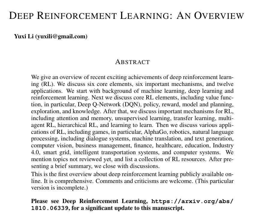
We give an overview of recent exciting achievements of deep reinforcement learning (RL). We discuss six core elements, six important mechanisms, and twelve applications. We start with background of machine learning, deep learning and reinforcement learning. Next we discuss core RL elements, including value function, in particular, Deep Q-Network (DQN), policy, reward, model, planning, and exploration. After that, we discuss important mechanisms for RL, including attention and memory, unsupervised learning, transfer learning, multi-agent RL, hierarchical RL, and learning to learn. Then we discuss various applications of RL, including games, in particular, AlphaGo, robotics, natural language processing, including dialogue systems, machine translation, and text generation, computer vision, neural architecture design, business management, finance, healthcare, Industry 4.0, smart grid, intelligent transportation systems, and computer systems. We mention topics not reviewed yet, and list a collection of RL resources. After presenting a brief summary, we close with discussions.

Please see Deep Reinforcement Learning, arXiv:1810.06339, for a significant update.

Table of Contents

  • 1 Introduction
  • 2 Background
  • 2.1 Machine Learning
  • 2.2 Deep Learning
  • 2.3 Reinforcement Learning
  • 2.3.1 Problem Setup
  • 2.3.2 Exploration vs Exploitation
  • 2.3.3 Value Function
  • 2.3.4 Dynamic Programming
  • 2.3.5 Temporal Difference Learning
  • 2.3.6 Multi-step Bootstrapping
  • 2.3.7 Function Approximation
  • 2.3.8 Policy Optimization
  • 2.3.9 Deep Reinforcement Learning
  • 2.3.10 RL Parlance
  • 2.3.11 Brief Summary
  • 3 Core Elements
  • 3.1 Value Function
  • 3.1.1 Deep Q-Network (DQN) And Extensions
  • 3.2 Policy
  • 3.2.1 Actor-Critic
  • 3.2.2 Policy Gradient
  • 3.2.3 Combining Policy Gradient with Off-Policy RL
  • 3.3 Reward
  • 3.4 Model and Planning
  • 3.5 Exploration
  • 3.6 Knowledge
  • 4 Important Mechanisms
  • 4.1 Attention and Memory
  • 4.2 Unsupervised Learning
  • 4.2.1 Horde
  • 4.2.2 Unsupervised Auxiliary Learning
  • 4.2.3 Generative Adversarial Networks
  • 4.3 Transfer Learning
  • 4.4 Multi-Agent Reinforcement Learning
  • 4.5 Hierarchical Reinforcement Learning
  • 4.6 Learning to Learn
  • 4.6.1 Learning to Learn/Optimize
  • 4.6.2 Zero/One/Few-Shot Learning
  • 4.6.3 Neural Architecture Design
  • 5 Applications
  • 5.1 Games
  • 5.1.1 Perfect Information Board Games
  • 5.1.2 Imperfect Information Board Games
  • 5.1.3 Video Games
  • 5.2 Robotics
  • 5.2.1 Guided Policy Search
  • 5.2.2 Learn to Navigate
  • 5.3 Natural Language Processing
  • 5.3.1 Dialogue Systems
  • 5.3.2 Machine Translation
  • 5.3.3 Text Generation
  • 5.4 Computer Vision
  • 5.4.1 Background
  • 5.4.2 Recognition
  • 5.4.3 Motion Analysis
  • 5.4.4 Scene Understanding
  • 5.4.5 Integration with NLP
  • 5.4.6 Visual Control
  • 5.5 Business Management
  • 5.6 Finance
  • 5.7 Healthcare
  • 5.8 Education
  • 5.9 Industry 4.0
  • 5.10 Smart Grid
  • 5.11 Intelligent Transportation Systems
  • 5.12 Computer Systems
  • 5.12.1 Resource Allocation
  • 5.12.2 Performance Optimization
  • 5.12.3 Security & Privacy
  • 6 More Topics
  • 7 Resources
  • 7.1 Books
  • 7.2 More Books
  • 7.3 Surveys and Reports
  • 7.4 Courses
  • 7.5 Tutorials
  • 7.6 Conferences, Journals and Workshops
  • 7.7 Blogs
  • 7.8 Testbeds
  • 7.9 Algorithm Implementations
  • 8 Brief Summary
  • 9 Discussions
  • References

Knowls

  1. Knowl 1 — Deep Q-Network Algorithm

    algorithm

    The Deep Q-Network (DQN) algorithm trains a deep convolutional neural network to approximate optimal action-values Q(s,a;θ)Q(s, a; \theta) directly from high-dimensional sensory observations. DQN stabilizes non-linear deep reinforcement learning via two core mechanisms: an experience replay memory DD that breaks correlations between successive transitions and smooths the data distribution, and a separate target network Q^\hat{Q} with parameters θ\theta^- updated periodically to provide stationary temporal difference targets.

    Input: Raw observation sequences, replay buffer capacity NN, discount factor γ(0,1]\gamma \in (0, 1], target network update period CC, exploration parameter ϵ\epsilon.
    Output: Optimal action-value function parameter vector θ\theta.
    Initialize replay memory DD to capacity NN
    Initialize action-value network QQ with random weights θ\theta
    Initialize target network Q^\hat{Q} with weights θ=θ\theta^- = \theta
    for episode =1= 1 to MM do
        Initialize sequence s1={x1}s_1 = \{x_1\} and preprocessed representation ϕ1=ϕ(s1)\phi_1 = \phi(s_1)
        for t=1t = 1 to TT do
            With probability ϵ\epsilon select random action atAa_t \in \mathcal{A}, otherwise select at=argmaxaQ(ϕ(st),a;θ)a_t = \arg\max_a Q(\phi(s_t), a; \theta)
            Execute action ata_t, observe reward rtr_t and next observation xt+1x_{t+1}
            Set st+1=st,at,xt+1s_{t+1} = s_t, a_t, x_{t+1} and compute ϕt+1=ϕ(st+1)\phi_{t+1} = \phi(s_{t+1})
            Store transition tuple (ϕt,at,rt,ϕt+1)(\phi_t, a_t, r_t, \phi_{t+1}) in replay memory DD
            
            Sample random minibatch of transitions (ϕj,aj,rj,ϕj+1)(\phi_j, a_j, r_j, \phi_{j+1}) from DD
            if episode terminates at step j+1j+1 then
                Set yj=rjy_j = r_j
            else
                Set yj=rj+γmaxaQ^(ϕj+1,a;θ)y_j = r_j + \gamma \max_{a'} \hat{Q}(\phi_{j+1}, a'; \theta^-)
            end if
            
            Perform gradient descent step on (yjQ(ϕj,aj;θ))2(y_j - Q(\phi_j, a_j; \theta))^2 with respect to parameters θ\theta
            Every CC steps, reset target network weights θ=θ\theta^- = \theta
        end for
    end for
  2. Knowl 2 — Asynchronous Advantage Actor-Critic Algorithm

    algorithm

    Asynchronous Advantage Actor-Critic (A3C) uses multiple parallel worker threads running on a single multi-core CPU, each interacting with an independent environment replica. By executing diverse exploration policies across parallel threads, A3C decorrelates agent experience without requiring an experience replay buffer. Each worker accumulates policy and value function gradients over nn-step forward trajectories and asynchronously updates global shared parameter vectors θ\theta and θv\theta_v.

    Input: Global shared policy parameters θ\theta, global shared value parameters θv\theta_v, global step counter T=0T = 0, global step limit TmaxT_{\max}, trajectory length tmaxt_{\max}, discount factor γ\gamma.
    Output: Trained global shared parameters θ\theta and θv\theta_v.
    Initialize thread step counter t1t \leftarrow 1
    while TTmaxT \le T_{\max} do
        Reset thread gradients dθ0d\theta \leftarrow 0 and dθv0d\theta_v \leftarrow 0
        Synchronize thread parameters θ=θ\theta' = \theta and θv=θv\theta'_v = \theta_v
        Set tstart=tt_{\text{start}} = t, acquire initial state sts_t
        while sts_t is not terminal and ttstart<tmaxt - t_{\text{start}} < t_{\max} do
            Select action atπ(atst;θ)a_t \sim \pi(a_t | s_t; \theta')
            Execute action ata_t, observe reward rtr_t and next state st+1s_{t+1}
            tt+1t \leftarrow t + 1
            TT+1T \leftarrow T + 1
        end while
        
        if sts_t is terminal then
            R=0R = 0
        else
            R=V(st;θv)R = V(s_t; \theta'_v)
        end if
        
        for i=t1i = t - 1 down to tstartt_{\text{start}} do
            Rri+γRR \leftarrow r_i + \gamma R
            dθdθ+θlogπ(aisi;θ)(RV(si;θv))d\theta \leftarrow d\theta + \nabla_{\theta'} \log \pi(a_i | s_i; \theta')(R - V(s_i; \theta'_v))
            dθvdθv+θv(RV(si;θv))2d\theta_v \leftarrow d\theta_v + \nabla_{\theta'_v} (R - V(s_i; \theta'_v))^2
        end for
        
        Asynchronously update global θ\theta using dθd\theta, and global θv\theta_v using dθvd\theta_v
    end while
  3. Knowl 3 — AlphaGo Zero Self-Play and Training Pipeline

    algorithm

    AlphaGo Zero implements approximate policy iteration without human demonstration or handcrafted features. A dual-headed deep neural network fθ(s)=(p,v)f_\theta(s) = (\mathbf{p}, v) outputs move probabilities p\mathbf{p} and position evaluation v[1,1]v \in [-1, 1] directly from raw board representations. Monte Carlo Tree Search (APV-MCTS) functions as a policy improvement operator to compute improved move distributions π\pi, while self-play games generate sample outcomes z{1,+1}z \in \{-1, +1\} for policy evaluation. The network is optimized end-to-end to align move probabilities p\mathbf{p} with search policies π\pi and scalar values vv with actual winners zz.

    Input: Raw board state ss, search budget NsimN_{\text{sim}}, temperature τ\tau, weight regularization hyperparameter cc.
    Output: Value-policy network parameters θ\theta.
    Initialize network parameters θ0\theta_0 randomly
    for each iteration i=1,2,i = 1, 2, \dots do
        Initialize starting state s0s_0
        for step t=0,1,t = 0, 1, \dots until game termination at step TT do
            Run MCTS using network fθi1f_{\theta_{i-1}} from root sts_t:
            while search budget remains do
                Select edge with maximum Q(s,a)+U(s,a)Q(s, a) + U(s, a), where U(s,a)P(s,a)/(1+N(s,a))U(s, a) \propto P(s, a)/(1 + N(s, a))
                Expand leaf node sLs_L and evaluate (P(sL,),V(sL))=fθi1(sL)(P(s_L, \cdot), V(s_L)) = f_{\theta_{i-1}}(s_L)
                Backup tree: increment visit counts N(s,a)N(s, a) and update action values Q(s,a)Q(s, a) to mean evaluations
            end while
            Compute search policy πt(a)N(st,a)1/τ\pi_t(a) \propto N(s_t, a)^{1/\tau}
            Sample action atπta_t \sim \pi_t, transition to st+1s_{t+1}
        end for
        Score game to obtain final outcome rT{1,+1}r_T \in \{-1, +1\}
        For each step tt, assign player outcome zt=±rTz_t = \pm r_T
        Store transition tuples (st,πt,zt)(s_t, \pi_t, z_t) in self-play memory
        Sample minibatch (s,π,z)(s, \pi, z) uniformly from self-play memory
        Update parameters θi\theta_i via gradient descent on loss: l=(zv)2πlogp+cθ2l = (z - v)^2 - \pi^\top \log \mathbf{p} + c \|\theta\|^2
        Evaluate updated model against previous best player to decide model promotion
    end for
  4. Knowl 4 — Double Q-Learning Value Correction for Deep RL

    model/method

    Standard Q-learning and DQN suffer from systematic overestimation bias due to using the max\max operator simultaneously for action selection and action evaluation in the target computation:

    ytQ=rt+1+γQ(st+1,argmaxaQ(st+1,a;θt);θt)y_t^Q = r_{t+1} + \gamma Q(s_{t+1}, \arg\max_a Q(s_{t+1}, a; \theta_t); \theta_t)

    Double DQN (D-DQN) decouples these operations by using the online network parameters θt\theta_t to greedily select the action and the target network parameters θt\theta_t^- to evaluate the value of that selected action:

    ytD-DQN=rt+1+γQ(st+1,argmaxaQ(st+1,a;θt);θt)y_t^{D\text{-}DQN} = r_{t+1} + \gamma Q\left(s_{t+1}, \arg\max_a Q(s_{t+1}, a; \theta_t); \theta_t^-\right)

    This target formulation mitigates over-optimistic value estimates without changing the underlying network architecture.

  5. Knowl 5 — Dueling Network Architecture for Q-Value Decomposition

    model/method

    The dueling network architecture decomposes the state-action value function Q(s,a)Q(s, a) into a state value function V(s)V(s) and a state-dependent action advantage function A(s,a)A(s, a). Convolutional layers output a shared feature representation, which feeds two separate streams of fully connected layers parameterized by β\beta (for VV) and α\alpha (for AA).

    To ensure identifiability and numerical stability, the streams are combined by subtracting the mean advantage across all actions in state ss:

    Q(s,a;θ,α,β)=V(s;θ,β)+(A(s,a;θ,α)1AaAA(s,a;θ,α))Q(s, a; \theta, \alpha, \beta) = V(s; \theta, \beta) + \left( A(s, a; \theta, \alpha) - \frac{1}{|\mathcal{A}|} \sum_{a' \in \mathcal{A}} A(s, a'; \theta, \alpha) \right)

    where θ\theta represents shared parameters. This allows the network to learn state values directly without needing to estimate the effect of every individual action at each state.

  6. Knowl 6 — Generative Adversarial Imitation Learning

    model/method

    Generative Adversarial Imitation Learning (GAIL) bypasses intermediate inverse reinforcement learning (IRL) steps to extract policies directly from expert demonstration trajectories. GAIL frames imitation learning as a two-player minimax game between a discriminator DR:S(0,1)D_R: \mathcal{S} \to (0, 1) and a policy generator πθ\pi_\theta:

    minπθmaxDREπθ[logDR(s)]+EπE[log(1DR(s))]\min_{\pi_\theta} \max_{D_R} \mathbb{E}_{\pi_\theta}[\log D_R(s)] + \mathbb{E}_{\pi_E}[\log(1 - D_R(s))]

    which can be written equivalently as:

    maxπθminDREπθ[logDR(s)]EπE[log(1DR(s))]\max_{\pi_\theta} \min_{D_R} -\mathbb{E}_{\pi_\theta}[\log D_R(s)] - \mathbb{E}_{\pi_E}[\log(1 - D_R(s))]

    The discriminator is optimized with supervised cross-entropy loss to differentiate state distributions produced by the expert policy πE\pi_E from those produced by πθ\pi_\theta. The policy πθ\pi_\theta is trained via policy optimization algorithms (such as Trust Region Policy Optimization) using logDR(s)-\log D_R(s) as the surrogate reward signal, converging when the generated distribution is indistinguishable from expert demonstrations (DR(s)=0.5D_R(s) = 0.5).

  7. Knowl 7 — Theoretical Properties and Convergence of Temporal Difference Algorithms

    data/table

    The deadly triad in reinforcement learning refers to the instability and potential divergence that occurs when combining function approximation, bootstrapping, and off-policy learning. The comparative theoretical and computational properties of temporal difference learning algorithms under these settings are summarized below:

    Algorithm Linear Computation Nonlinear Convergent Off-Policy Convergent Model-Free, Online Converges to PBE=0\text{PBE} = 0
    TD(λ\lambda) / SARSA(λ\lambda)
    ADP
    LSTD(λ\lambda) / LSPE(λ\lambda)
    Fitted-Q
    Residual Gradient
    GTD(λ\lambda) / GQ(λ\lambda)

    Here, Linear Computation indicates linear per-step time and memory complexity; Nonlinear Convergent denotes guaranteed convergence under nonlinear function approximation; Off-Policy Convergent denotes guaranteed convergence when target and behavior policies differ; Model-Free, Online indicates execution without transition models on incremental stream data; and Converges to PBE=0\text{PBE}=0 indicates convergence to a solution satisfying zero Projected Bellman Error.

  8. Knowl 8 — REINFORCE Algorithm with Value Function Baseline

    algorithm

    REINFORCE with baseline is an episodic Monte Carlo policy gradient algorithm. To reduce gradient variance while preserving unbiasedness, a parameterized state-value function baseline v^(st,w)\hat{v}(s_t, w) is subtracted from the empirical discounted return GtG_t.

    Input: Differentiable policy π(as;θ)\pi(a|s; \theta), differentiable state-value baseline v^(s,w)\hat{v}(s, w), step sizes α>0\alpha > 0, β>0\beta > 0, discount factor γ(0,1]\gamma \in (0, 1].
    Output: Optimized policy parameter vector θ\theta.
    Initialize policy parameter vector θ\theta and state-value weight vector ww arbitrarily
    for each episode do
        Generate trajectory s0,a0,r1,s1,a1,,sT1,aT1,rTs_0, a_0, r_1, s_1, a_1, \dots, s_{T-1}, a_{T-1}, r_T following π(;θ)\pi(\cdot | \cdot; \theta)
        for t=0t = 0 to T1T - 1 do
            Gtk=t+1Tγkt1rkG_t \leftarrow \sum_{k=t+1}^T \gamma^{k - t - 1} r_k
            δGtv^(st,w)\delta \leftarrow G_t - \hat{v}(s_t, w)
            ww+βδwv^(st,w)w \leftarrow w + \beta \delta \nabla_w \hat{v}(s_t, w)
            θθ+αγtδθlogπ(atst;θ)\theta \leftarrow \theta + \alpha \gamma^t \delta \nabla_\theta \log \pi(a_t | s_t; \theta)
        end for
    end for
  9. Knowl 9 — One-Step Episodic Actor-Critic Algorithm

    algorithm

    The one-step actor-critic algorithm combines policy optimization with temporal difference bootstrapping. The critic maintains a state-value approximation v^(s,w)\hat{v}(s, w) to compute the one-step TD error δ\delta, which updates critic weights ww and provides an estimated advantage to guide gradient ascent updates for the actor policy parameters θ\theta.

    Input: Differentiable policy π(as;θ)\pi(a|s; \theta), differentiable state-value function v^(s,w)\hat{v}(s, w) with v^(terminal,w)=0\hat{v}(\text{terminal}, w) = 0, step sizes α>0\alpha > 0, β>0\beta > 0, discount factor γ(0,1]\gamma \in (0, 1].
    Output: Policy parameter vector θ\theta and value parameter vector ww.
    Initialize policy parameters θ\theta and value weights ww arbitrarily
    for each episode do
        Initialize starting state ss
        I1I \leftarrow 1
        while ss is not terminal do
            Sample action aπ(s;θ)a \sim \pi(\cdot | s; \theta)
            Take action aa, observe scalar reward rr and next state ss'
            δr+γv^(s,w)v^(s,w)\delta \leftarrow r + \gamma \hat{v}(s', w) - \hat{v}(s, w)
            ww+βδwv^(s,w)w \leftarrow w + \beta \delta \nabla_w \hat{v}(s, w)
            θθ+αIδθlogπ(as;θ)\theta \leftarrow \theta + \alpha I \delta \nabla_\theta \log \pi(a | s; \theta)
            IγII \leftarrow \gamma I
            sss \leftarrow s'
        end while
    end for
  10. Knowl 10 — Taxonomy of Deep Reinforcement Learning Challenges and Solution Mechanisms

    model/method

    Deep reinforcement learning research is systematically structured around fundamental challenges and their modern algorithmic solutions:

    1. Value Function Evaluation and Control: Temporal difference learning addresses policy evaluation; Q-learning, SARSA, and policy gradient methods handle optimal control.
    2. Deadly Triad Instability: Mitigated by DQN (replay buffers and target networks), Double DQN (decoupled action evaluation), Dueling architectures (value-advantage separation), A3C (asynchronous parallel execution), and Gradient-TD/Emphatic-TD methods.
    3. Sample/Data Efficiency: Addressed via model-based policy search (PILCO), actor-critic experience replay (ACER), hybrid off-policy/policy-gradient architectures (PGQ, Q-Prop), and return-based off-policy operators (Retrace, Reactor).
    4. Unavailable Reward Functions: Solved through inverse reinforcement learning, learning from demonstrations (DQfD), and adversarial imitation learning (GAIL).
    5. Exploration-Exploitation Tradeoff: Addressed via pseudo-counts unifying count-based exploration and intrinsic motivation, under-appreciated reward exploration, bootstrapped DQN, and parameter-space noise (NoisyNet).
    6. Model-Free Planning: Solved by embedding planning operations into differentiable neural architectures (Value Iteration Networks, Predictron).
    7. Lifelong and Multi-Task Generalization: Addressed through hierarchical reinforcement learning (options, feudal networks, STRAW), external differentiable memory (DNC), and meta-learning / learning-to-learn frameworks.

Coverage note — Omitted extensive bibliographic cataloging of external domain applications (such as computer vision tasks, smart grid systems, healthcare records, and finance setups) and lists of online resources/courses from Sections 5, 6, and 7, as they summarize literature rather than introducing primary methods or theory.

References

  1. 1.Abadi, M., Chu, A., Goodfellow, I., McMahan, H. B., Mironov, I., Talwar, K., and Zhang, L. (2016). Deep learning with differential privacy. In ACM Conference on Computer and Communications Security (ACM CCS).
  2. 2.Abbeel, P. and Ng, A. Y. (2004). Apprenticeship learning via inverse reinforcement learning. In the International Conference on Machine Learning (ICML).
  3. 3.Agrawal, P., Nair, A., Abbeel, P., Malik, J., and Levine, S. (2016). Learning to poke by poking: Experiential learning of intuitive physics. In the Annual Conference on Neural Information Processing Systems (NIPS).
  4. 4.Al-Shedivat, M., Bansal, T., Burda, Y., Sutskever, I., Mordatch, I., and Abbeel, P. (2017a). Continuous Adaptation via Meta-Learning in Nonstationary and Competitive Environments. ArXiv e-prints.
  5. 5.Al-Shedivat, M., Dubey, A., and Xing, E. P. (2017b). Contextual Explanation Networks. ArXiv e-prints.
  6. 6.Albrechta, S. V. and Stone, P. (2018). Autonomous agents modelling other agents: A comprehensive survey and open problems. Artificial Intelligence.
  7. 7.Alsheikh, M. A., Lin, S., Niyato, D., and Tan, H.-P. (2014). Machine learning in wireless sensor networks: Algorithms, strategies, and applications. IEEE Communications Surveys & Tutorials, 16(4):1996–2018.
  8. 8.Amin, K., Jiang, N., and Singh, S. (2017). Repeated inverse reinforcement learning. In the Annual Conference on Neural Information Processing Systems (NIPS).
  9. 9.Amodei, D., Olah, C., Steinhardt, J., Christiano, P., Schulman, J., and Mane, D. (2016). Concrete Problems in AI Safety. ArXiv e-prints.
  10. 10.Anderson, H. S., Kharkar, A., Filar, B., and Roth, P. (2017). Evading machine learning malware detection. In Black Hat USA.
  11. 11.Anderson, R. N., Boulanger, A., Powell, W. B., and Scott, W. (2011). Adaptive stochastic control for the smart grid. Proceedings of the IEEE, 99(6):1098–1115.
  12. 12.Andreas, J., Klein, D., and Levine, S. (2017). Modular multitask reinforcement learning with policy sketches. In the International Conference on Machine Learning (ICML).
  13. 13.Andrychowicz, M., Denil, M., Colmenarejo, S. G., Hoffman, M. W., Pfau, D., Schaul, T., Shillingford, B., and de Freitas, N. (2016). Learning to learn by gradient descent by gradient descent. In the Annual Conference on Neural Information Processing Systems (NIPS).
  14. 14.Andrychowicz, M., Wolski, F., Ray, A., Schneider, J., Fong, R., Welinder, P., McGrew, B., Tobin, J., Abbeel, P., and Zaremba, W. (2017). Hindsight experience replay. In the Annual Conference on Neural Information Processing Systems (NIPS).
  15. 15.Anschel, O., Baram, N., and Shimkin, N. (2017). Averaged-DQN: Variance reduction and stabilization for deep reinforcement learning. In the International Conference on Machine Learning (ICML).
  16. 16.Argall, B. D., Chernova, S., Veloso, M., and Browning, B. (2009). A survey of robot learning from demonstration. Robotics and Autonomous Systems, 57(5):469–483.
  17. 17.Arjovsky, M., Chintala, S., and Bottou, L. (2017). Wasserstein GAN. ArXiv e-prints.
  18. 18.Artetxe, M., Labaka, G., Agirre, E., and Cho, K. (2017). Unsupervised Neural Machine Translation. ArXiv e-prints.
  19. 19.Arulkumaran, K., Deisenroth, M. P., Brundage, M., and Bharath, A. A. (2017). A Brief Survey of Deep Reinforcement Learning. ArXiv e-prints.
  20. 20.Asri, L. E., He, J., and Suleman, K. (2016). A sequence-to-sequence model for user simulation in spoken dialogue systems. In Annual Meeting of the International Speech Communication Association (INTERSPEECH).

Citation

MLA
Li, Y. “Deep Reinforcement Learning: An Overview”. arXiv, 2017, http://arxiv.org/abs/1701.07274v6.
APA
Li, Y. (2017). Deep Reinforcement Learning: An Overview. arXiv. http://arxiv.org/abs/1701.07274v6
Chicago
Li, Y. 2017. “Deep Reinforcement Learning: An Overview”. arXiv. http://arxiv.org/abs/1701.07274v6.
Harvard
Li, Y. (2017) “Deep Reinforcement Learning: An Overview”, arXiv [Preprint]. Available at: http://arxiv.org/abs/1701.07274v6.
Vancouver
1. Li Y (2017) Deep Reinforcement Learning: An Overview. arXiv

BibTeX

@article{li2017deep,
  title = {Deep Reinforcement Learning: An Overview},
  author = {Li, Yuxi},
  year = {2017},
  journal = {arXiv},
  url = {http://arxiv.org/abs/1701.07274v6},
  eprint = {1701.07274}
}
Metadata:arXiv

Access the Paper

This paper is available from its original source. Click below to access the PDF.

Open PDF

License: Authors