Deep Recurrent Q-Learning for Partially Observable MDPs

Matthew HausknechtPeter Stone

article2015AAAI2,004 citations

Introduces Deep Recurrent Q-Networks by integrating an LSTM into standard Deep Q-Networks, demonstrating that recurrent memory allows reinforcement learning agents to handle partially observable environments and better adapt to degraded visual inputs than traditional frame-stacking methods.

Listen

Real-world autonomous systems and decision-making controllers frequently operate in noisy, uncertain environments where sensors provide incomplete state information. Standard deep reinforcement learning methods, such as the standard Deep Q-Network, assume full observability by feeding a short, fixed history of recent frames directly into the network. This approach fails to handle conditions where essential data is obscured or requires longer-term memory. The article addresses this operational vulnerability by evaluating whether integrating recurrent memory allows reinforcement learning controllers to maintain performance under partial observability.

The article set out to demonstrate whether adding a recurrent Long Short-Term Memory layer to a deep Q-learning architecture enables an agent to integrate visual observations across time and better handle environments with incomplete state information. To evaluate this approach, the authors modified the standard Deep Q-Network into a Deep Recurrent Q-Network by replacing its first fully connected layer with a recurrent memory layer. They evaluated this framework across nine standard Atari video games and artificially induced partial observability using a flickering setting where screen frames were obscured with a 50 percent probability. Training utilized randomized mini-batches from replay memory with ten unrolled timesteps across ten million iterations per task.

The findings show that the recurrent network matches standard baseline performance across fully observable games despite processing only a single frame per timestep rather than a four-frame stack. In specific environments, such as Frostbite and Double Dunk, the recurrent network outperformed the standard baseline, achieving a score of 2,875 compared to 519 in Frostbite. Furthermore, when trained under full visibility and evaluated across environments with increasing degrees of obscured frames, the recurrent controller degraded significantly less than the standard baseline, retaining a higher percentage of its original score across all levels of missing information. However, across standard benchmarks as a whole, the recurrent network showed no systematic advantage over simple frame stacking, and in some games, like Beam Rider, it scored less than half of the baseline.

These results demonstrate that recurrent memory functions as a robust alternative to stacking fixed frame histories, providing greater resilience when observation quality degrades at deployment time. For decision-makers, choosing a recurrent architecture represents an effective strategy to mitigate operational risks in dynamic environments where sensor streams may drop frames or suffer intermittent occlusions. While recurrency does not provide universal performance gains, its ability to generalize from clean training data to degraded operational conditions makes it a safer architecture for real-world deployment.

Organizations deploying visual reinforcement learning systems in noisy or variable sensor conditions should consider recurrent architectures when operational observability cannot be guaranteed. However, engineering teams should evaluate specific task dynamics before deployment, as stacking frames remains simpler and computationally lighter for static, fully observable tasks. Future work should focus on identifying domain characteristics that favor recurrent architectures and exploring architectures with higher memory capacities without incurring excessive computational training overhead.

Readers should note that the evaluation is limited to a benchmark suite of nine arcade games and synthetic flickering conditions rather than physical real-world sensory inputs. Additionally, training recurrent architectures requires substantially higher compute time, with deeper sequence unrolling increasing computational burden significantly. Confidence remains high that recurrent networks improve robustness under observational degradation, but caution is warranted before expecting universal score improvements across all task domains.

University of Texas at Austin computer games deep reinforcement learning frames Recurrent Deep Games

arXiv: 1507.06527

Paper: Human-level control through deep reinforcement learning, Volodymyr Mnih et al. (2015). This seminal paper introduces the Deep Q-Network (DQN) architecture and experience replay mechanism that the source directly augments with recurrent LSTM layers.
Paper: Playing Atari with Deep Reinforcement Learning, Volodymyr Mnih et al. (2013). This work establishes learning policies directly from raw Atari pixel frames via stacked observations, defining the baseline approach that the source aims to improve upon under partial observability.
Paper: Long Short-Term Memory, Sepp Hochreiter et al. (1997). This foundation paper introduces Long Short-Term Memory (LSTM) recurrent networks, which the source integrates into DQN to maintain memory over time.
Paper: Technical Note: Q-Learning, CHRISTOPHER J.C.H. WATKINS et al. (2004). This paper establishes the mathematical formulation and convergence proof of model-free Q-learning that forms the theoretical backbone of the source's reinforcement learning method.
Paper: Long-term Recurrent Convolutional Networks for Visual Recognition and Description, Jeff Donahue et al. (2015). This work details the architectural integration of convolutional visual encoders with recurrent LSTM layers to process temporal visual sequences.
Paper: On the difficulty of training recurrent neural networks, Razvan Pascanu et al. (2012). This analysis of gradient difficulties and training dynamics in recurrent networks provides vital context for understanding how recurrent layers behave during backpropagation through time.
Paper: Learning to Predict by the Methods of Temporal Differences, Richard S. Sutton (1988). This foundational text introduces temporal-difference learning methods, which underpin the value updates used in deep Q-learning.
Paper: Reinforcement Learning: A Survey, Leslie Pack Kaelbling et al. (1996). This classic survey provides essential conceptual foundations on Markov decision processes and reinforcement learning principles.

Paper: Recurrent Experience Replay in Distributed Reinforcement Learning, Steven Kapturowski et al. (2019). This paper directly extends recurrent deep Q-learning to distributed systems with prioritized experience replay by addressing recurrent state staleness and initialization.
Paper: Asynchronous Methods for Deep Reinforcement Learning, Volodymyr Mnih et al. (2016). This work builds on deep reinforcement learning across Atari benchmarks by introducing asynchronous parallel actor architectures that incorporate recurrent LSTM policies.
Paper: Learning to Navigate in Complex Environments, Piotr Mirowski et al. (2017). This paper applies recurrent deep reinforcement learning architectures to solve partially observable 3D navigation tasks using auxiliary predictive objectives.
Paper: Reinforcement Learning with Unsupervised Auxiliary Tasks, Max Jaderberg et al. (2017). This work enhances recurrent deep RL architectures with unsupervised auxiliary sensorimotor tasks to accelerate learning under sparse reward signals.
Paper: Rainbow: Combining Improvements in Deep Reinforcement Learning, Matteo Hessel et al. (2017). This benchmark work synthesizes subsequent key innovations in value-based deep reinforcement learning beyond standard DQN.
Paper: Deep Reinforcement Learning with Double Q-learning, Hado van Hasselt et al. (2016). This article addresses severe value overestimation in deep Q-learning by introducing Double DQN, improving the stability of Q-value estimation.
Paper: Prioritized Experience Replay, Tom Schaul et al. (2016). This research introduces prioritized experience replay, replacing the uniform replay sampling strategy utilized in standard and recurrent DQNs.
Paper: Dueling Network Architectures for Deep Reinforcement Learning, Ziyu Wang et al. (2016). This paper develops the dueling network architecture to factor state value and action advantages, offering a complementary structural improvement over standard deep Q-networks.
Paper: A Brief Survey of Deep Reinforcement Learning, Kai Arulkumaran et al. (2017). This survey provides a comprehensive synthesis of the evolution of deep reinforcement learning paradigms, placing recurrent Q-learning within the broader landscape.

Cover for Deep Recurrent Q-Learning for Partially Observable MDPs

Abstract

Deep Reinforcement Learning has yielded proficient controllers for complex tasks. However, these controllers have limited memory and rely on being able to perceive the complete game screen at each decision point. To address these shortcomings, this article investigates the effects of adding recurrency to a Deep Q-Network (DQN) by replacing the first post-convolutional fully-connected layer with a recurrent LSTM. The resulting \textit{Deep Recurrent Q-Network} (DRQN), although capable of seeing only a single frame at each timestep, successfully integrates information through time and replicates DQN's performance on standard Atari games and partially observed equivalents featuring flickering game screens. Additionally, when trained with partial observations and evaluated with incrementally more complete observations, DRQN's performance scales as a function of observability. Conversely, when trained with full observations and evaluated with partial observations, DRQN's performance degrades less than DQN's. Thus, given the same length of history, recurrency is a viable alternative to stacking a history of frames in the DQN's input layer and while recurrency confers no systematic advantage when learning to play the game, the recurrent net can better adapt at evaluation time if the quality of observations changes.

Introduction
Deep Q-Learning
Partial Observability
DRQN Architecture
Stable Recurrent Updates
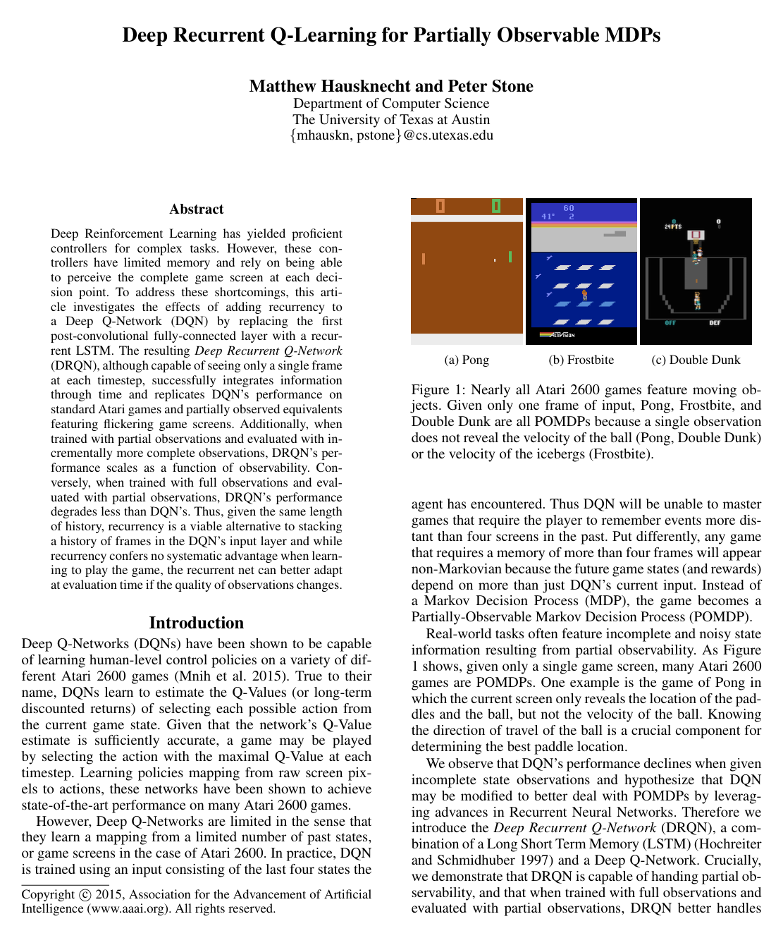
Atari Games: MDP or POMDP?
Flickering Atari Games
Evaluation on Standard Atari Games
MDP to POMDP Generalization
Related Work
Discussion and Conclusion
Acknowledgments
References
A Appendix A: Alternative Architectures
B Appendix B: Computational Efficiency
C Appendix C: Experimental Details
D Appendix C: Flickering Results

Knowls

Knowl 1 — Deep Recurrent Q-Network (DRQN) Architecture
model/method
The Deep Recurrent Q-Network (DRQN) adapts the Deep Q-Network (DQN) architecture to partially observable environments by replacing the first post-convolutional fully connected layer with a recurrent Long Short-Term Memory (LSTM) layer.

The input to DRQN is a single preprocessed grayscale frame of dimensions $84 \times 84 \times 1$ , rather than a stack of four history frames as in standard DQN. The network architecture consists of:
1. Convolutional Layer 1: 32 filters of size $8 \times 8$ with stride 4.
2. Convolutional Layer 2: 64 filters of size $4 \times 4$ with stride 2.
3. Convolutional Layer 3: 64 filters of size $3 \times 3$ with stride 1.
4. Recurrent Layer: An LSTM layer containing 512 hidden units, which directly receives the flattened feature activations from the third convolutional layer.
5. Output Layer: A fully connected linear layer mapping the 512-dimensional LSTM output at each timestep to estimated action values $Q(o_t, a; \theta)$ for each available action $a \in \mathcal{A}$ .
All parameters across the convolutional and recurrent layers are learned jointly from scratch via end-to-end backpropagation through time.
Knowl 2 — Bootstrapped Random Updates for Recurrent Deep Q-Learning
algorithm
Training recurrent neural networks with experience replay requires specific update strategies to handle temporal dependencies across sequential observations. While Bootstrapped Sequential Updates sample full episodes and carry hidden states forward across the entire sequence (violating uniform transition sampling), Bootstrapped Random Updates sample truncated sub-sequences and zero the initial recurrent state.
Input: Replay memory $\mathcal{D}$ , main Q-network parameters $\theta$ , target Q-network parameters $\theta^-$ , unroll length $L=10$ , learning rate $\alpha$ , discount factor $\gamma$
Output: Updated network parameters $\theta$
Sample an episode $E = (o_1, a_1, r_1, o_2, \dots, o_T)$ uniformly at random from $\mathcal{D}$
Select a start index $t \in \{1, \dots, T - L\}$ uniformly at random
Initialize LSTM hidden state $h_{t-1} \leftarrow 0$ and cell state $c_{t-1} \leftarrow 0$
Initialize target LSTM hidden state $\hat{h}_{t-1} \leftarrow 0$ and cell state $\hat{c}_{t-1} \leftarrow 0$
for $\tau = t$ to $t + L - 1$ do
    Compute Q-values: $Q(o_\tau, \cdot; \theta), (h_\tau, c_\tau) \leftarrow \text{DRQN}(o_\tau, h_{\tau-1}, c_{\tau-1}; \theta)$
    Compute target Q-values: $\hat{Q}(o_{\tau+1}, \cdot; \theta^-), (\hat{h}_\tau, \hat{c}_\tau) \leftarrow \text{DRQN}(o_{\tau+1}, \hat{h}_{\tau-1}, \hat{c}_{\tau-1}; \theta^-)$
    if episode terminates at $\tau + 1$ then
         $y_\tau \leftarrow r_\tau$
    else
         $y_\tau \leftarrow r_\tau + \gamma \max_{a'} \hat{Q}(o_{\tau+1}, a'; \theta^-)$
    end if
    Compute loss component: $\mathcal{L}_\tau(\theta) = (y_\tau - Q(o_\tau, a_\tau; \theta))^2$
end for
Compute gradient $\nabla_\theta \sum_{\tau=t}^{t+L-1} \mathcal{L}_\tau(\theta)$ using Backpropagation Through Time over $L$ steps
Clip LSTM gradients to a maximum norm/value of 10.0
Update parameters $\theta$ via ADADELTA optimizer
Empirical evaluation demonstrates that both sequential updates and random updates converge to policies with similar performance across Atari games. Bootstrapped random updates are preferred in practice due to lower complexity and alignment with experience replay sampling.
Knowl 3 — Flickering Atari POMDP Formulation
experimental setup
To evaluate reinforcement learning algorithms under partial observability without altering internal game dynamics, the Flickering Atari POMDP protocol modifies the Arcade Learning Environment visual stream.

At each timestep $t$ , given the true underlying console screen $s_t$ , the observation $o_t$ emitted to the agent is stochastically corrupted according to an obscuration probability $p \in [0, 1)$ :

$o_t = \begin{cases} s_t & \text{with probability } 1 - p \\ \mathbf{0} & \text{with probability } p \end{cases}$

where $\mathbf{0}$ represents a completely obscured (blank) screen. In the default Flickering Atari benchmark, $p = 0.5$ , meaning that on average half of all game frames are obscured. To succeed, an agent must integrate observations across non-contiguous frames to estimate velocities, positions, and trajectories of game objects.
Knowl 4 — MDP-to-POMDP Zero-Shot Generalization
empirical result
When policies are trained on standard, fully observable Atari 2600 games (where the observation probability $p_{\text{obs}} = 1.0$ ) and evaluated on flickering POMDP variants with varying observation probabilities $p_{\text{obs}} \in [0.1, 0.9]$ , DRQN demonstrates greater robustness than DQN.

Across 9 evaluated Atari games (Asteroids, Beam Rider, Bowling, Centipede, Chopper Command, Double Dunk, Frostbite, Ice Hockey, Ms. Pacman):
- Both architectures suffer performance degradation as observation quality decreases ( $p_{\text{obs}} \to 0$ ).
- DRQN retains a consistently higher percentage of its baseline fully observed score across all values of $p_{\text{obs}}$ . For instance, at $p_{\text{obs}} = 0.5$ , DRQN retains roughly $50\%$ of its original performance compared to approximately $30\%$ for DQN.
This indicates that incorporating recurrency provides innate robustness against missing or intermittent sensory data at test time, even when the agent was never exposed to partial observability during training.

Knowl 5 — Performance Comparison on Standard Atari 2600 Games

data/table

Performance of 1-frame DRQN compared against 4-frame DQN across 9 standard Atari games (evaluated with fully observed screens, where 4-frame history renders the games effectively MDPs).

Game	DRQN $\pm$ std	DQN (Ours) $\pm$ std	DQN (Mnih et al.) $\pm$ std
Asteroids	$1020\;(\pm 312)$	$1070\;(\pm 345)$	$1629\;(\pm 542)$
Beam Rider	$3269\;(\pm 1167)$	$\mathbf{6923\;(\pm 1027)}$	$6846\;(\pm 1619)$
Bowling	$62\;(\pm 5.9)$	$72\;(\pm 11)$	$42\;(\pm 88)$
Centipede	$3534\;(\pm 1601)$	$3653\;(\pm 1903)$	$8309\;(\pm 5237)$
Chopper Command	$2070\;(\pm 875)$	$1460\;(\pm 976)$	$6687\;(\pm 2916)$
Double Dunk	$\mathbf{-2\;(\pm 7.8)}$	$-10\;(\pm 3.5)$	$-18.1\;(\pm 2.6)$
Frostbite	$\mathbf{2875\;(\pm 535)}$	$519\;(\pm 363)$	$328.3\;(\pm 250.5)$
Ice Hockey	$-4.4\;(\pm 1.6)$	$-3.5\;(\pm 3.5)$	$-1.6\;(\pm 2.5)$
Ms. Pacman	$2048\;(\pm 653)$	$2363\;(\pm 735)$	$2311\;(\pm 525)$

Bold values indicate statistically significant differences between DRQN and the replicated DQN ( $p < .05$ , Benjamini-Hochberg procedure). DRQN significantly outperforms DQN on Frostbite and Double Dunk, performs similarly on five games, and achieves significantly lower scores on Beam Rider.

Knowl 6 — Performance Comparison on Flickering Atari 2600 POMDPs

data/table

Performance of 1-frame DRQN versus 4-frame DQN across 10 Atari games under the flickering POMDP condition, where each frame is obscured with probability $p = 0.5$ .

Flickering Game	DRQN $\pm$ std	DQN $\pm$ std
Asteroids	$1032\;(\pm 410)$	$1010\;(\pm 535)$
Beam Rider	$618\;(\pm 115)$	$\mathbf{1685.6\;(\pm 875)}$
Bowling	$65.5\;(\pm 13)$	$57.3\;(\pm 8)$
Centipede	$4319.2\;(\pm 4378)$	$5268.1\;(\pm 2052)$
Chopper Command	$1330\;(\pm 294)$	$1450\;(\pm 787.8)$
Double Dunk	$-14\;(\pm 2.5)$	$-16.2\;(\pm 2.6)$
Frostbite	$414\;(\pm 494)$	$436\;(\pm 462.5)$
Ice Hockey	$-5.4\;(\pm 2.7)$	$-4.2\;(\pm 1.5)$
Ms. Pacman	$1739\;(\pm 942)$	$1824\;(\pm 490)$
Pong	$\mathbf{12.1\;(\pm 2.2)}$	$-9.9\;(\pm 3.3)$

Bold values denote statistical significance ( $p < .05$ ). On Flickering Pong, DRQN substantially outperforms DQN ( $+12.1$ vs $-9.9$ ). However, across the remaining games, DRQN does not show a systematic advantage over DQN, and DQN achieves significantly higher scores on Flickering Beam Rider.

Knowl 7 — Temporal Feature Integration: Recurrent LSTM vs. Convolutional Stacking
empirical result
Visualizing layer activations reveals distinct mechanisms for temporal feature integration between non-recurrent frame-stacked DQNs and single-frame DRQNs:
1. Convolutional Frame Stacking (10-frame DQN): Early convolutional filters (Conv1) detect static object positions (e.g., paddle). Deeper convolutional filters (Conv2, Conv3) act as spatio-temporal velocity detectors, firing in response to directional ball motion, speed, and paddle-ball interactions.
2. Recurrent Integration (1-frame DRQN): Because DRQN receives only a single $84 \times 84$ frame per step, its convolutional layers cannot compute motion or velocity. Instead, convolutional filters extract purely spatial features, and temporal integration occurs within the LSTM layer. Individual LSTM units specialize to detect high-level temporal game events across time, including the agent missing the ball, ball reflections off paddles, and ball deflections off walls.

Knowl 8 — Architectural Placement of Recurrent Layers

empirical result

Evaluation of alternative recurrent placements and activation structures on Beam Rider demonstrates that directly replacing the first fully connected layer (IP1) with an LSTM yields the strongest performance:

Key structural findings:

Placing the LSTM directly after the convolutional layers (LSTM replaces IP1) performs better than inserting the LSTM after a dense layer (LSTM over IP1), hypothesized to be due to direct recurrent access to spatial feature maps.
Placing a Rectified Linear Unit (ReLU) activation immediately after the LSTM layer consistently reduces agent performance.
Combining input frame stacking (4 stacked frames) with temporal LSTM unrolling (10 steps) increases parameter count and compute time without improving performance, likely due to overfitting.

Knowl 9 — Computational Efficiency and Runtime Scaling of DRQN

data/table

Forward and backward pass processing times measured over 1,000 iterations on an Nvidia GTX Titan Black with CuDNN and Caffe:

	Backwards (ms)			Forwards (ms)
Input Frames	1	4	10	1	4	10
Baseline (Non-recurrent DQN)	$8.82$	$13.6$	$26.7$	$2.0$	$4.0$	$9.0$
LSTM Unroll 1	$18.2$	$22.3$	$33.7$	$2.4$	$4.4$	$9.4$
LSTM Unroll 10	$77.3$	$111.3$	$180.5$	$2.5$	$4.4$	$8.3$
LSTM Unroll 30	$204.5$	$263.4$	$491.1$	$2.5$	$3.8$	$9.4$

Computation scales sub-linearly with the number of input channels and unroll steps. While forward pass times remain nearly flat across unroll depths ( $ildeline 2.4\text{--}9.4\text{ ms}$ ), backward pass times increase substantially with the unroll depth (e.g., $77.3\text{ ms}$ for 10-step unroll vs $204.5\text{ ms}$ for 30-step unroll at 1 input frame). Unrolling 30 steps with 10 stacked frames would require over 56 days of training time to reach 10 million iterations.

Knowl 10 — Hyperparameters and Training Configuration for DRQN
experimental setup
DRQN training uses the following hyperparameter configuration:
- Replay Memory: Capacity of 400,000 transitions.
- Training Duration: 10,000,000 iterations.
- Optimizer: ADADELTA with learning rate $\alpha = 0.1$ and momentum $\rho = 0.95$ .
- Gradient Clipping: LSTM gradients are clipped to a maximum magnitude of $10.0$ .
- Target Network Update Period: Target network parameters $\theta^-$ are synchronized with main network parameters $\theta$ every 10,000 iterations.
- BPTT Unroll Length: 10 timesteps per gradient update.
- Evaluation Protocol: Evaluated every 50,000 iterations by averaging scores over 10 test episodes.
- Arcade Learning Environment (ALE) Options: Color averaging, minimal action set, and death detection.

Coverage note — No substantial contributed material was omitted. The knowls cover the network architecture, update algorithms, Flickering Atari POMDP benchmark, standard and flickering experimental results, layer placement ablations, temporal feature visualizations, computational profiling, and training hyperparameters.

References

1.Bakker, B. 2001. Reinforcement learning with long short-term memory. In NIPS, 1475–1482. MIT Press.
2.Bellemare, M. G.; Naddaf, Y.; Veness, J.; and Bowling, M. 2013. The arcade learning environment: An evaluation platform for general agents. Journal of Artificial Intelligence Research 47:253–279.
3.Cun, Y. L. L.; Bottou, L.; Bengio, Y.; and Haffner, P. 1998. Gradient-based learning applied to document recognition. Proceedings of IEEE 86(11):2278–2324.
4.Guo, X.; Singh, S.; Lee, H.; Lewis, R. L.; and Wang, X. 2014. Deep learning for real-time atari game play using offline monte-carlo tree search planning. In Ghahramani, Z.; Welling, M.; Cortes, C.; Lawrence, N.; and Weinberger, K., eds., Advances in Neural Information Processing Systems 27. Curran Associates, Inc. 3338–3346.
5.Hochreiter, S., and Schmidhuber, J. 1997. Long short-term memory. Neural Comput. 9(8):1735–1780.
6.Jia, Y.; Shelhamer, E.; Donahue, J.; Karayev, S.; Long, J.; Girshick, R.; Guadarrama, S.; and Darrell, T. 2014. Caffe: Convolutional architecture for fast feature embedding. arXiv preprint arXiv:1408.5093.
7.Karpathy, A.; Johnson, J.; and Li, F.-F. 2015. Visualizing and understanding recurrent networks. arXiv preprint.
8.Mnih, V.; Kavukcuoglu, K.; Silver, D.; Rusu, A. A.; Veness, J.; Bellemare, M. G.; Graves, A.; Riedmiller, M.; Fidjeland, A. K.; Ostrovski, G.; Petersen, S.; Beattie, C.; Sadik, A.; Antonoglou, I.; King, H.; Kumaran, D.; Wierstra, D.; Legg, S.; and Hassabis, D. 2015. Human-level control through deep reinforcement learning. Nature 518(7540):529–533.
9.Narasimhan, K.; Kulkarni, T.; and Barzilay, R. 2015. Language understanding for text-based games using deep reinforcement learning. CoRR abs/1506.08941.
10.Sutton, R. S., and Barto, A. G. 1998. Reinforcement Learning: An Introduction. MIT Press.
11.Tieleman, T., and Hinton, G. 2012. Lecture 6.5—RmsProp: Divide the gradient by a running average of its recent magnitude. COURSERA: Neural Networks for Machine Learning.
12.Tsitsiklis, J. N., and Roy, B. V. 1997. An analysis of temporal-difference learning with function approximation. IEEE Transactions on Automatic Control 42(5):674–690.
13.Watkins, C. J. C. H., and Dayan, P. 1992. Q-learning. Machine Learning 8(3-4):279–292.
14.Wierstra, D.; Foerster, A.; Peters, J.; and Schmidthuber, J. 2007. Solving deep memory POMDPs with recurrent policy gradients.
15.Zeiler, M. D. 2012. ADADELTA: An adaptive learning rate method. CoRR abs/1212.5701.

Citation

MLA

Hausknecht, M., and P. Stone. “Deep Recurrent Q-Learning for Partially Observable MDPs”. arXiv, 2015, http://arxiv.org/abs/1507.06527v4.

APA

Hausknecht, M., & Stone, P. (2015). Deep Recurrent Q-Learning for Partially Observable MDPs. arXiv. http://arxiv.org/abs/1507.06527v4

Chicago

Hausknecht, M., and P. Stone. 2015. “Deep Recurrent Q-Learning for Partially Observable MDPs”. arXiv. http://arxiv.org/abs/1507.06527v4.

Harvard

Hausknecht, M. and Stone, P. (2015) “Deep Recurrent Q-Learning for Partially Observable MDPs”, arXiv [Preprint]. Available at: http://arxiv.org/abs/1507.06527v4.

Vancouver

1. Hausknecht M, Stone P (2015) Deep Recurrent Q-Learning for Partially Observable MDPs. arXiv

BibTeX

@article{hausknecht2015deep,
  title = {Deep Recurrent Q-Learning for Partially Observable MDPs},
  author = {Hausknecht, Matthew and Stone, Peter},
  year = {2015},
  journal = {arXiv},
  url = {http://arxiv.org/abs/1507.06527v4},
  eprint = {1507.06527}
}

Metadata:arXiv

Access the Paper

This paper is available from its original source. Click below to access the PDF.

Open PDF

Architecture Description	Percent Improvement
LSTM replaces IP1	$709\%$
ReLU-LSTM replaces IP1	$533\%$
LSTM over IP1	$418\%$
ReLU-LSTM over IP1	$0\%$

Deep Recurrent Q-Learning for Partially Observable MDPs

Abstract

Topics

Keywords

Table of Contents

Knowls

Knowl 1 — Deep Recurrent Q-Network (DRQN) Architecture

Knowl 2 — Bootstrapped Random Updates for Recurrent Deep Q-Learning

Knowl 3 — Flickering Atari POMDP Formulation

Knowl 4 — MDP-to-POMDP Zero-Shot Generalization

Knowl 5 — Performance Comparison on Standard Atari 2600 Games

Knowl 6 — Performance Comparison on Flickering Atari 2600 POMDPs

Knowl 7 — Temporal Feature Integration: Recurrent LSTM vs. Convolutional Stacking

Knowl 8 — Architectural Placement of Recurrent Layers

Knowl 9 — Computational Efficiency and Runtime Scaling of DRQN

Knowl 10 — Hyperparameters and Training Configuration for DRQN

References

Citation

BibTeX

Access the Paper