
On the difficulty of training Recurrent Neural Networks
Razvan Pascanu
Universite de Montreal
[email protected]
Tomas Mikolov
Brno University
[email protected]
Yoshua Bengio
Universite de Montreal
[email protected]
Keywords: recurrent neural networks, vanishing gradients, exploding gradients
Abstract
There are two widely known issues with properly training Recurrent Neural Networks, the vanishing and the exploding gradient problems detailed in [1]. In this paper we attempt to improve the understanding of the underlying issues by exploring these problems from an analytical, a geometric and a dynamical systems perspective. Our analysis is used to justify a simple yet effective solution. We propose a gradient norm clipping strategy to deal with exploding gradients and a soft constraint for the vanishing gradients problem. We validate empirically our hypothesis and proposed solutions in the experimental section.
Executive Summary: The paper examines why recurrent neural networks (RNNs) remain difficult to train for tasks involving time series or sequential data. RNNs can in principle capture long-range temporal dependencies through recurrent connections in their hidden state, yet in practice gradient-based training often fails because gradients either grow exponentially large or shrink exponentially fast as they are propagated backward through many time steps. This instability blocks effective learning of correlations that span dozens or hundreds of steps.
The authors set out to clarify the mechanisms behind these exploding and vanishing gradients and to derive practical remedies. They combine an analytical treatment of the product of Jacobian matrices that appear in back-propagation through time, a geometric view of the resulting error surface, and a dynamical-systems perspective that links gradient explosions to crossings between basins of attraction. They then test the resulting algorithms on both synthetic “pathological” benchmarks that require long memory and on real tasks such as polyphonic music prediction and character-level language modeling.
The analysis shows that gradients explode when the largest absolute eigenvalue of the recurrent weight matrix exceeds a threshold set by the derivative bound of the activation function, and vanish when it falls below that threshold. The geometry of the error surface contains steep “walls” aligned with the exploding directions; a conventional gradient step therefore tends to overshoot narrow valleys and derail training. Empirically, simply rescaling the gradient vector whenever its norm exceeds a modest threshold restores stable progress and yields 100 % success on sequences up to length 200 where plain stochastic gradient descent fails entirely. Adding a soft regularization term that encourages the relevant Jacobian factors to preserve norm further improves the capture of long-range dependencies. On music and language benchmarks the combined procedure produces statistically significant reductions in negative log-likelihood relative to unregularized baselines and matches or exceeds earlier state-of-the-art RNN results.
These findings matter because the proposed fixes are inexpensive, require only one extra hyper-parameter (the clipping threshold), and can be applied on top of existing optimizers. They therefore lower the barrier to using RNNs on any sequential problem where long-term structure is relevant. The methods also generalize: models trained on sequences of length 200 often continue to perform well on sequences twice as long.
The main limitations are that the theoretical guarantees assume bounded activation derivatives and do not cover chaotic regimes, and that the regularization coefficient still needs modest per-task tuning. Practitioners should therefore monitor gradient norms during early training to set the clipping threshold and should view the regularization term as an optional but low-cost lever when long-range dependencies dominate the task.
1. Introduction
Section Summary: Recurrent neural networks are models designed to handle time-series data by adding connections in the hidden layer that carry information forward from one time step to the next, allowing the network to capture patterns that may span many steps. Although this structure makes them well suited for sequential tasks, they are difficult to train in practice because gradients can vanish or explode when errors are propagated backward through many time steps. The section outlines how backpropagation through time is used to compute these gradients and reframes the calculations to show how individual contributions from distant versus recent time steps affect learning.
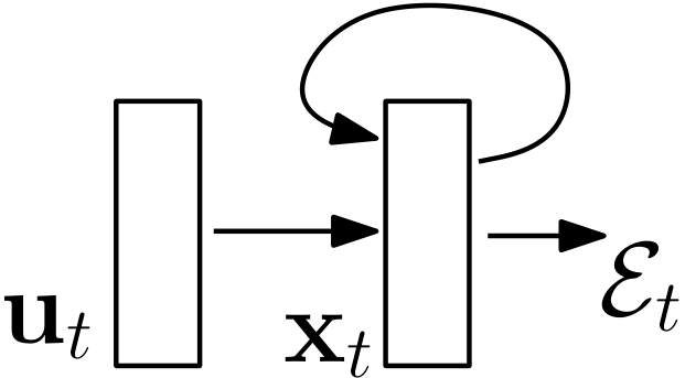
A recurrent neural network (RNN), e.g. Figure 1, is a neural network model proposed in the 80's ([2, 3, 4]) for modeling time series. The structure of the network is similar to that of a standard multilayer perceptron, with the distinction that we allow connections among hidden units associated with a time delay. Through these connections the model can retain information about the past inputs, enabling it to discover temporal correlations between events that are possibly far away from each other in the data (a crucial property for proper learning of time series).
 {width=20%}
While in principle the recurrent network is a simple and powerful model, in practice, it is unfortunately hard to train properly. Among the main reasons why this model is so unwieldy are the vanishing gradient and exploding gradient problems described in [1].
1.1 Training recurrent networks
A generic recurrent neural network, with input $\mathbf{u}_t$ and state $\mathbf{x}_t$ for time step $t$, is given by equation 1. In the theoretical section of this paper we will sometimes make use of the specific parametrization given by equation 2 [^1] in order to provide more precise conditions and intuitions about the everyday use-case.
[^1]: This formulation is equivalent to the more widely known equation $\mathbf{x}{t} = \sigma(\mathbf{W}{rec} \mathbf{x}{t-1} + \mathbf{W}{in} \mathbf{u}_t + \mathbf{b})$, and it was chosen for convenience.
$ \mathbf{x}t = F(\mathbf{x}{t-1}, \mathbf{u}_{t}, \theta)\tag{1} $
$ \mathbf{x}{t} = \mathbf{W}{rec} \sigma(\mathbf{x}{t-1}) + \mathbf{W}{in} \mathbf{u}_{t} + \mathbf{b}\tag{2} $
The parameters of the model are given by the recurrent weight matrix $\mathbf{W}{rec}$, the biases $\mathbf{b}$ and input weight matrix $\mathbf{W}{in}$, collected in $\theta$ for the general case. $\mathbf{x}{0}$ is provided by the user, set to zero or learned, and $\sigma$ is an element-wise function (usually the tanh or sigmoid). A cost $\mathcal{E}$ measures the performance of the network on some given task and it can be broken apart into individual costs for each step $\mathcal{E} = \sum{1 \leq t \leq T}\mathcal{E}_t$, where $\mathcal{E}t = \mathcal{L}(\mathbf{x}{t})$.
One approach that can be used to compute the necessary gradients is Backpropagation Through Time (BPTT), where the recurrent model is represented as a deep multi-layer one (with an unbounded number of layers) and backpropagation is applied on the unrolled model (see Figure 2).
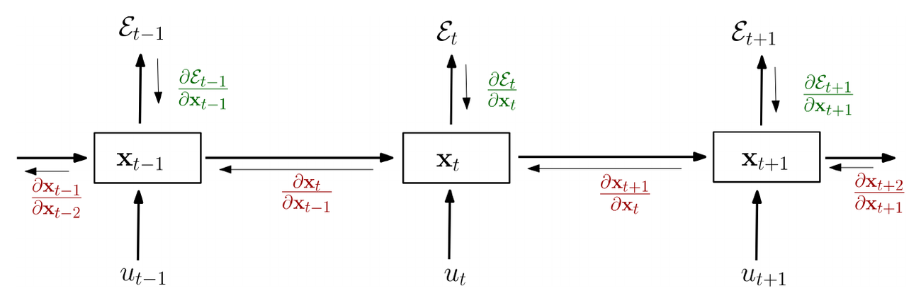
We will diverge from the classical BPTT equations at this point and re-write the gradients (see equations 3, Equation 4 and 5) in order to better highlight the exploding gradients problem. These equations were obtained by writing the gradients in a sum-of-products form.
$ \frac{\partial \mathcal{E}}{\partial \theta} = \sum_{1 \leq t \leq T} \frac{\partial \mathcal{E}_t}{\partial \theta}\tag{3} $
$ \frac{\partial \mathcal{E}t}{\partial \theta} = \sum{1 \leq k \leq t} \left(\frac{\partial \mathcal{E}t}{\partial \mathbf{x}{t}} \frac{\partial \mathbf{x}{t}}{\partial \mathbf{x}{k}} \frac{\partial^+ \mathbf{x}{_{k}}}{\partial \theta} \right)\tag{4} $
$ \frac{\partial \mathbf{x}{t}}{\partial \mathbf{x}{k}}= \prod_{t \geq i > k} \frac{\partial \mathbf{x}i}{\partial \mathbf{x}{i-1}} = \prod_{t \geq i > k} \mathbf{W}{rec}^T diag (\sigma'(\mathbf{x}{i-1}))\tag{5} $
$\frac{\partial^+ \mathbf{x}{{k}}}{\partial \theta}$ refers to the "immediate" partial derivative of the state $\mathbf{x}k$ with respect to $\theta$, i.e., where $\mathbf{x}{k-1}$ is taken as a constant with respect to $\theta$. Specifically, considering equation 2, the value of any row $i$ of the matrix $(\frac{\partial^+ \mathbf{x}k}{\partial \mathbf{W}{rec}})$ is just $\sigma(\mathbf{x}{k-1})$. Equation 5 also provides the form of Jacobian matrix $\frac{\partial \mathbf{x}i}{\partial \mathbf{x}{i-1}}$ for the specific parametrization given in equation 2, where $diag$ converts a vector into a diagonal matrix, and $\sigma'$ computes the derivative of $\sigma$ in an element-wise fashion.
Note that each term $\frac{\partial \mathcal{E}_t}{\partial \theta}$ from equation 3 has the same form and the behaviour of these individual terms determine the behaviour of the sum. Henceforth we will focus on one such generic term, calling it simply the gradient when there is no confusion.
Any gradient component $\frac{\partial \mathcal{E}t}{\partial \theta}$ is also a sum (see equation 4), whose terms we refer to as temporal contributions or temporal components. One can see that each such temporal contribution $\frac{\partial \mathcal{E}t}{\partial \mathbf{x}{t}} \frac{\partial \mathbf{x}{t}}{\partial \mathbf{x}{k}} \frac{\partial^+ \mathbf{x}{{k}}}{\partial \theta}$ measures how $\theta$ at step $k$ affects the cost at step $t>k$. The factors $\frac{\partial \mathbf{x}{t}}{\partial \mathbf{x}{k}}$ (equation 5) transport the error "in time" from step $t$ back to step $k$. We would further loosely distinguish between long term and short term contributions, where long term refers to components for which $k \ll t$ and short term to everything else.
2. Exploding and Vanishing Gradients
Section Summary: In recurrent neural networks, the gradients used for training can explode in size or shrink to zero because each one is formed by multiplying many Jacobian matrices across time steps, just as repeated multiplication of numbers can grow without bound or decay to nothing. This causes long-term components to dominate or disappear exponentially, so the model struggles to learn connections between events separated by many steps. The problems occur when the largest eigenvalue of the recurrent weight matrix falls below or rises above a threshold set by the activation function's slope, and they also arise from abrupt shifts in the network's dynamical attractors.
As introduced in [1], the exploding gradients problem refers to the large increase in the norm of the gradient during training. Such events are caused by the explosion of the long term components, which can grow exponentially more then short term ones. The vanishing gradients problem refers to the opposite behaviour, when long term components go exponentially fast to norm 0, making it impossible for the model to learn correlation between temporally distant events.
2.1 The mechanics
To understand this phenomenon we need to look at the form of each temporal component, and in particular at the matrix factors $\frac{\partial \mathbf{x}_t}{\partial \mathbf{x}_k}$ (see equation 5) that take the form of a product of $t-k$ Jacobian matrices. In the same way a product of $t-k$ real numbers can shrink to zero or explode to infinity, so does this product of matrices (along some direction $\mathbf{v}$).
In what follows we will try to formalize these intuitions (extending a similar derivation done in [1] where only a single hidden unit case was considered).
If we consider a linear version of the model (i.e. set $\sigma$ to the identity function in equation 2) we can use the power iteration method to formally analyze this product of Jacobian matrices and obtain tight conditions for when the gradients explode or vanish (see the supplementary materials for a detailed derivation of these conditions). It is sufficient for the largest eigenvalue $\lambda_1$ of the recurrent weight matrix to be smaller than 1 for long term components to vanish (as $t \to \infty$) and necessary for it to be larger than 1 for gradients to explode.
We can generalize these results for nonlinear functions $\sigma$ where the absolute values of $\sigma'(x)$ is bounded (say by a value $\gamma \in \mathcal{R}$) and therefore $\left|diag(\sigma'(\mathbf{x}_k))\right| \leq \gamma$.
We first prove that it is sufficient for $\lambda_1 < \frac{1}{\gamma}$, where $\lambda_1$ is the absolute value of the largest eigenvalue of the recurrent weight matrix $\mathbf{W}{rec}$, for the vanishing gradient problem to occur. Note that we assume the parametrization given by equation 2. The Jacobian matrix $\frac{\partial \mathbf{x}{k+1}}{\partial \mathbf{x}k}$ is given by $\mathbf{W}{rec}^T {diag}(\sigma'(\mathbf{x}_k))$. The 2-norm of this Jacobian is bounded by the product of the norms of the two matrices (see equation 6). Due to our assumption, this implies that it is smaller than 1.
$ \forall k, \left|\frac{\partial \mathbf{x}{k+1}}{\partial \mathbf{x}{k}}\right| \leq \left|\mathbf{W}_{rec}^T\right|\left|{diag}(\sigma'(\mathbf{x}_k))\right| < \frac{1}{\gamma}\gamma < 1\tag{6} $
Let $\eta \in \mathrm{R}$ be such that $\forall k, \left|\frac{\partial \mathbf{x}{k+1}}{\partial \mathbf{x}{k}}\right| \leq \eta <1$. The existence of $\eta$ is given by equation 6. By induction over $i$, we can show that
$ \frac{\partial \mathcal{E}t}{\partial \mathbf{x}t} \left(\prod{i=k}^{t-1} \frac{\partial \mathbf{x}{i+1}}{\partial \mathbf{x}_i}\right) \leq \eta^{t-k} \frac{\partial \mathcal{E}_t}{\partial \mathbf{x}_t}\tag{7} $
As $\eta < 1$, it follows that, according to equation 7, long term contributions (for which $t-k$ is large) go to 0 exponentially fast with $t-k$. $\Box$
By inverting this proof we get the necessary condition for exploding gradients, namely that the largest eigenvalue $\lambda_1$ is larger than $\frac{1}{\gamma}$ (otherwise the long term components would vanish instead of exploding). For $\tanh$ we have $\gamma=1$ while for sigmoid we have $\gamma = \kern.1em^{1}\kern-.3em/\kern-.1em_{4}$.
2.2 Drawing similarities with Dynamical Systems
We can improve our understanding of the exploding gradients and vanishing gradients problems by employing a dynamical systems perspective, as it was done before in [5, 6].
We recommend reading [7] for a formal and detailed treatment of dynamical systems theory. For any parameter assignment $\theta$, depending on the initial state $\mathbf{x}_0$, the state $\mathbf{x}_t$ of an autonomous dynamical system converges, under the repeated application of the map $F$, to one of several possible different attractor states (e.g. point attractors, though other type of attractors exist). The model could also find itself in a chaotic regime, case in which some of the following observations may not hold, but that is not treated in depth here. Attractors describe the asymptotic behaviour of the model. The state space is divided into basins of attraction, one for each attractor. If the model is started in one basin of attraction, the model will converge to the corresponding attractor as $t$ grows.
Dynamical systems theory tells us that as $\theta$ changes slowly, the asymptotic behaviour changes smoothly almost everywhere except for certain crucial points where drastic changes occur (the new asymptotic behaviour ceases to be topologically equivalent to the old one). These points are called bifurcation boundaries and are caused by attractors that appear, disappear or change shape.
[5] hypothesizes that such bifurcation crossings could cause the gradients to explode. We would like to extend this observation into a sufficient condition for gradients to explode, and for that reason we will re-use the one-hidden unit model (and plot) from [5] (see Figure 3).
The x-axis covers the parameter $b$ and the y-axis the asymptotic state $\mathbf{x}\infty$. The bold line follows the movement of the final point attractor, $\mathbf{x}\infty$, as $b$ changes. At $b_1$ we have a bifurcation boundary where a new attractor emerges (when $b$ decreases from $\infty$), while at $b_2$ we have another that results in the disappearance of one of the two attractors. In the interval $(b_1, b_2)$ we are in a rich regime, where there are two attractors and the change in position of boundary between them, as we change $b$, is traced out by a dashed line. The vector field (gray dashed arrows) describe the evolution of the state $\mathbf{x}$ if the network is initialized in that region.
![**Figure 3:** Bifurcation diagram of a single hidden unit RNN (with fixed recurrent weight of 5.0 and adjustable bias $b$; example introduced in [5]). See text.](https://ittowtnkqtyixxjxrhou.supabase.co/storage/v1/object/public/public-images/6k4ga4qj/complex_fig_80d9d118377c.png) {width=90%}
{width=90%}
We show that there are two types of events that could lead to a large change in $\mathbf{x}_t$, with $t\to\infty$. One is crossing a boundary between basins of attraction (depicted with a unfilled circles), while the other is crossing a bifurcation boundary (filled circles). For large $t$, the $\Delta x_t$ resulting from a change in $b$ will be large even for very small changes in $b$ (as the system is attracted towards different attractors) which leads to a large gradient.
It is however neither necessary nor sufficient to cross a bifurcation for the gradients to explode, as bifurcations are global events that could have no effect locally. Learning traces out a path in the parameter-state space. If we are at a bifurcation boundary, but the state of the model is such that it is in the basin of attraction of one attractor (from many possible attractors) that does not change shape or disappear when the bifurcation is crossed, then this bifurcation will not affect learning.
Crossing boundaries between basins of attraction is a local event, and it is sufficient for the gradients to explode. If we assume that crossing into an emerging attractor or from a disappearing one (due to a bifurcation) qualifies as crossing some boundary between attractors, that we can formulate a sufficient condition for gradients to explode which encapsulates the observations made in [5], extending them to also normal crossing of boundaries between different basins of attractions. Note how in the figure, there are only two values of $b$ with a bifurcation, but a whole range of values for which there can be a boundary crossing.
Another limitation of previous analysis is that they only consider autonomous systems and assume the observations hold for input-driven models. In [1] input is dealt with by assuming it is bounded noise. The downside of this approach is that it limits how one can reason about the input. In practice, the input is supposed to drive the dynamical system, being able to leave the model in some attractor state, or kick it out of the basin of attraction when certain triggering patterns present themselves.
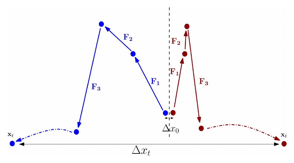
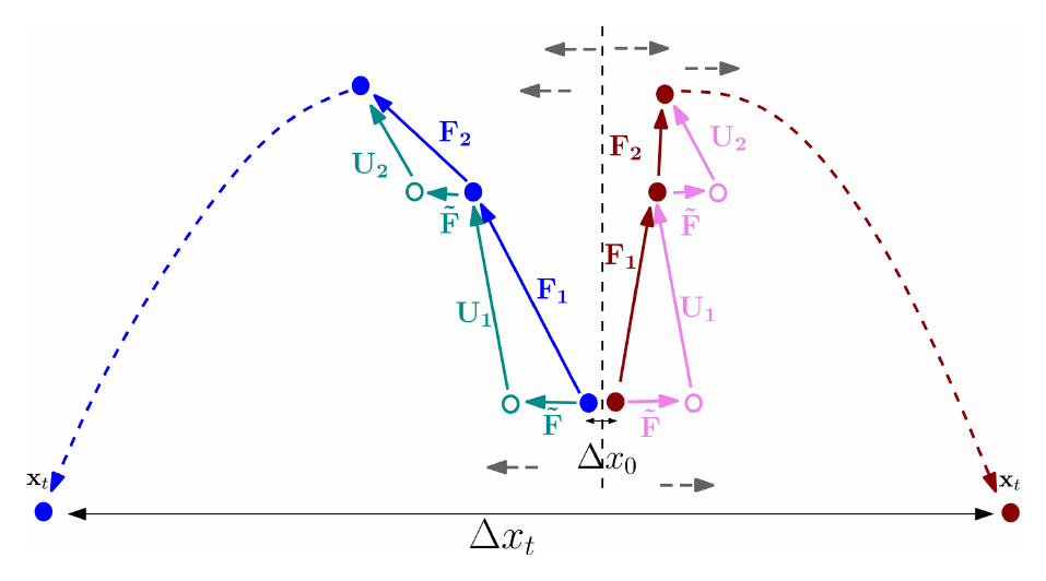
We propose to extend our analysis to input driven models by folding the input into the map. We consider the family of maps $F_t$, where we apply a different $F_t$ at each step. Intuitively, for the gradients to explode we require the same behaviour as before, where (at least in some direction) the maps $F_1, .., F_t$ agree and change direction. Figure 4 describes this behaviour.
 {width=70%}
For the specific parametrization provided by equation 2 we can take the analogy one step further by decomposing the maps $F_t$ into a fixed map $\tilde{F}$ and a time-varying one $U_t$. $F(\mathbf{x}) = \mathbf{W}{rec}\sigma(\mathbf{x}) +\mathbf{b}$ corresponds to an input-less recurrent network, while $U_t(\mathbf{x})= \mathbf{x} + \mathbf{W}{in}\mathbf{u}_t$ describes the effect of the input. This is depicted in in Figure 5. Since $U_t$ changes with time, it can not be analyzed using standard dynamical systems tools, but $\tilde{F}$ can. This means that when a boundary between basins of attractions is crossed for $\tilde{F}$, the state will move towards a different attractor, which for large $t$ could lead (unless the input maps $U_t$ are opposing this) to a large discrepancy in $\mathbf{x}_t$. Therefore studying the asymptotic behaviour of $\tilde{F}$ can provide useful information about where such events are likely to happen.
 {width=70%}
One interesting observation from the dynamical systems perspective with respect to vanishing gradients is the following. If the factors $\frac{\partial \mathbf{x}_t}{\partial \mathbf{x}_k}$ go to zero (for $t-k$ large), it means that $\mathbf{x}_t$ does not depend on $\mathbf{x}_k$ (if we change $\mathbf{x}_k$ by some $\Delta$, $\mathbf{x}_t$ stays the same). This translates into the model at $\mathbf{x}_t$ being close to convergence towards some attractor (which it would reach from anywhere in the neighbourhood of $\mathbf{x}_k$).
2.3 The geometrical interpretation
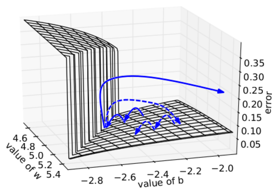
Let us consider a simple one hidden unit model (equation 8) where we provide an initial state $x_{0}$ and train the model to have a specific target value after 50 steps. Note that for simplicity we assume no input.
$ x_t = w \sigma(x_{t-1}) + b\tag{8} $
Figure 6 shows the error surface $\mathcal{E}{50} = (\sigma(x{50}) - 0.7)^2$, where $x_0 = .5$ and $\sigma$ to be the sigmoid function.
 {width=60%}
We can more easily analyze the behavior of this model by further simplifying it to be linear ($\sigma$ then being the identity function), with $b=0$. $x_t = x_0 w^t$ from which it follows that $\frac{\partial x_t}{\partial w} = tx_0w^{t-1}$ and $\frac{\partial^2 x_t}{\partial w^2} = t(t-1)x_0 w^{t-2}$, implying that when the first derivative explodes, so does the second derivative.
In the general case, when the gradients explode they do so along some directions $\mathbf{v}$. This says that there exists, in such situations, a vector $\mathbf{v}$ such that $\frac{\partial \mathcal{E}t}{\partial \theta} \mathbf{v} \geq C\alpha^t$, where $C, \alpha \in \mathrm{R}$ and $\alpha > 1$. For the linear case ($\sigma$ is the identity function), $\mathbf{v}$ is the eigenvector corresponding to the largest eigenvalue of $\mathbf{W}{rec}$. If this bound is tight, we hypothesize that in general when gradients explode so does the curvature along $\mathbf{v}$, leading to a wall in the error surface, like the one seen in Figure 6.
If this holds, then it gives us a simple solution to the exploding gradients problem depicted in Figure 6.
If both the gradient and the leading eigenvector of the curvature are aligned with the exploding direction $\mathbf{v}$, it follows that the error surface has a steep wall perpendicular to $\mathbf{v}$ (and consequently to the gradient). This means that when stochastic gradient descent (SGD) reaches the wall and does a gradient descent step, it will be forced to jump across the valley moving perpendicular to the steep walls, possibly leaving the valley and disrupting the learning process.
The dashed arrows in Figure 6 correspond to ignoring the norm of this large step, ensuring that the model stays close to the wall. The key insight is that all the steps taken when the gradient explodes are aligned with $\mathbf{v}$ and ignore other descent direction (i.e. the model moves perpendicular to the wall). At the wall, a small-norm step in the direction of the gradient therefore merely pushes us back inside the smoother low-curvature region besides the wall, whereas a regular gradient step would bring us very far, thus slowing or preventing further training. Instead, with a bounded step, we get back in that smooth region near the wall where SGD is free to explore other descent directions.
The important addition in this scenario to the classical high curvature valley, is that we assume that the valley is wide, as we have a large region around the wall where if we land we can rely on first order methods to move towards the local minima. This is why just clipping the gradient might be sufficient, not requiring the use a second order method. Note that this algorithm should work even when the rate of growth of the gradient is not the same as the one of the curvature (a case for which a second order method would fail as the ratio between the gradient and curvature could still explode).
Our hypothesis could also help to understand the recent success of the Hessian-Free approach compared to other second order methods. There are two key differences between Hessian-Free and most other second-order algorithms. First, it uses the full Hessian matrix and hence can deal with exploding directions that are not necessarily axis-aligned. Second, it computes a new estimate of the Hessian matrix before each update step and can take into account abrupt changes in curvature (such as the ones suggested by our hypothesis) while most other approaches use a smoothness assumption, i.e., averaging 2nd order signals over many steps.
3. Dealing with the exploding and vanishing gradient
Section Summary: Previous approaches to exploding and vanishing gradients in recurrent networks have included weight penalties to keep recurrent connections stable, specialized units like LSTMs that protect long-term information flow, teacher forcing during training, Hessian-based optimizers, and networks that leave recurrent weights untrained, though these often restrict what the model can learn or require extra setup. A straightforward alternative is to watch the overall size of the gradient at each step and rescale it down whenever it exceeds a chosen limit, which prevents sudden jumps in parameter updates while still moving in a useful direction. This clipping method is computationally cheap, draws from earlier practical tricks, and provides a more stable foundation for training on long sequences.
3.1 Previous solutions
Using an L1 or L2 penalty on the recurrent weights can help with exploding gradients. Given that the parameters initialized with small values, the spectral radius of $\mathbf{W}_{rec}$ is probably smaller than 1, from which it follows that the gradient can not explode (see necessary condition found in Section 2.1). The regularization term can ensure that during training the spectral radius never exceeds 1. This approach limits the model to a simple regime (with a single point attractor at the origin), where any information inserted in the model has to die out exponentially fast in time. In such a regime we can not train a generator network, nor can we exhibit long term memory traces.
[5] proposes to pre-program the model (to initialize the model in the right regime) or to use teacher forcing. The first proposal assumes that if the model exhibits from the beginning the same kind of asymptotic behaviour as the one required by the target, then there is no need to cross a bifurcation boundary. The downside is that one can not always know the required asymptotic behaviour, and, even if such information is known, it is not trivial to initialize a model in this specific regime. We should also note that such initialization does not prevent crossing the boundary between basins of attraction, which, as shown, could happen even though no bifurcation boundary is crossed.
Teacher forcing is a more interesting, yet a not very well understood solution. It can be seen as a way of initializing the model in the right regime and the right region of space. It has been shown that in practice it can reduce the chance that gradients explode, and even allow training generator models or models that work with unbounded amounts of memory([8, 9]). One important downside is that it requires a target to be defined at every time step.
In [10, 11] a solution is proposed for the vanishing gradients problem, where the structure of the model is changed. Specifically it introduces a special set of units called LSTM units which are linear and have a recurrent connection to itself which is fixed to 1. The flow of information into the unit and from the unit is guarded by an input and output gates (their behaviour is learned). There are several variations of this basic structure. This solution does not address explicitly the exploding gradients problem.
[12] use the Hessian-Free optimizer in conjunction with structural damping, a specific damping strategy of the Hessian. This approach seems to deal very well with the vanishing gradient, though more detailed analysis is still missing. Presumably this method works because in high dimensional spaces there is a high probability for long term components to be orthogonal to short term ones. This would allow the Hessian to rescale these components independently. In practice, one can not guarantee that this property holds. As discussed in Section 2.3, this method is able to deal with the exploding gradient as well. Structural damping is an enhancement that forces the change in the state to be small, when the parameter changes by some small value $\Delta \theta$. This asks for the Jacobian matrices $\frac{\partial \mathbf{x}_t}{\partial \theta}$ to have small norm, hence further helping with the exploding gradients problem. The fact that it helps when training recurrent neural models on long sequences suggests that while the curvature might explode at the same time with the gradient, it might not grow at the same rate and hence not be sufficient to deal with the exploding gradient.
Echo State Networks ([13]) avoid the exploding and vanishing gradients problem by not learning the recurrent and input weights. They are sampled from hand crafted distributions. Because usually the largest eigenvalue of the recurrent weight is, by construction, smaller than 1, information fed in to the model has to die out exponentially fast. This means that these models can not easily deal with long term dependencies, even though the reason is slightly different from the vanishing gradients problem. An extension to the classical model is represented by leaky integration units ([14]), where
$\mathbf{x}k= \alpha \mathbf{x}{k-1} + (1-\alpha) \sigma(\mathbf{W}{rec}\mathbf{x}{k-1} + \mathbf{W}_{in} \mathbf{u}_k + \mathbf{b})$.
While these units can be used to solve the standard benchmark proposed by [10] for learning long term dependencies (see [15]), they are more suitable to deal with low frequency information as they act as a low pass filter. Because most of the weights are randomly sampled, is not clear what size of models one would need to solve complex real world tasks.
We would make a final note about the approach proposed by Tomas Mikolov in his PhD thesis ([16])(and implicitly used in the state of the art results on language modelling ([17])). It involves clipping the gradient's temporal components element-wise (clipping an entry when it exceeds in absolute value a fixed threshold). Clipping has been shown to do well in practice and it forms the backbone of our approach.
3.2 Scaling down the gradients
As suggested in Section 2.3, one simple mechanism to deal with a sudden increase in the norm of the gradients is to rescale them whenever they go over a threshold (see Algorithm 1).
$\hat{\mathbf{g}} \leftarrow \frac{\partial \mathcal{E}}{\partial \theta}$
if $\|\hat{\mathbf{g}}\| \geq threshold$ then
  $\hat{\mathbf{g}} \leftarrow \frac{threshold}{\|\hat{\mathbf{g}} \|} \hat{\mathbf{g}}$
end if
This algorithm is very similar to the one proposed by Tomas Mikolov and we only diverged from the original proposal in an attempt to provide a better theoretical foundation (ensuring that we always move in a descent direction with respect to the current mini-batch), though in practice both variants behave similarly.
The proposed clipping is simple to implement and computationally efficient, but it does however introduce an additional hyper-parameter, namely the threshold. One good heuristic for setting this threshold is to look at statistics on the average norm over a sufficiently large number of updates. In our experiments we have noticed that for a given task and model size, training is not very sensitive to this hyper-parameter and the algorithm behaves well even for rather small thresholds.
The algorithm can also be thought of as adapting the learning rate based on the norm of the gradient. Compared to other learning rate adaptation strategies, which focus on improving convergence by collecting statistics on the gradient (as for example in [18], or [19] for an overview), we rely on the instantaneous gradient. This means that we can handle very abrupt changes in norm, while the other methods would not be able to do so.
3.3 Vanishing gradient regularization
We opt to address the vanishing gradients problem using a regularization term that represents a preference for parameter values such that back-propagated gradients neither increase or decrease too much in magnitude. Our intuition is that increasing the norm of $\frac{\partial \mathbf{x}_t}{\partial \mathbf{x}_k}$ means the error at time $t$ is more sensitive to all inputs $\mathbf{u}_t, .., \mathbf{u}_k$ ($\frac{\partial \mathbf{x}_t}{\partial \mathbf{x}_k}$ is a factor in $\frac{\partial \mathcal{E}_t}{\partial \mathbf{u}_k}$). In practice some of these inputs will be irrelevant for the prediction at time $t$ and will behave like noise that the network needs to learn to ignore. The network can not learn to ignore these irrelevant inputs unless there is an error signal. These two issues can not be solved in parallel, and it seems natural to expect that we need to force the network to increase the norm of $\frac{\partial \mathbf{x}_t}{\partial \mathbf{x}_k}$ at the expense of larger errors (caused by the irrelevant input entries) and then wait for it to learn to ignore these irrelevant input entries. This suggest that moving towards increasing the norm of $\frac{\partial \mathbf{x}_t}{\partial \mathbf{x}_k}$ can not be always done while following a descent direction of the error $\mathcal{E}$ (which is, for e.g., what a second order method would try to do), and therefore we need to enforce it via a regularization term.
The regularizer we propose below prefers solutions for which the error signal preserves norm as it travels back in time:
$ \Omega = \sum_k \Omega_k = \sum_k \left(\frac{ \left| \frac{\partial \mathcal{E}}{\partial \mathbf{x}{k+1}} \frac{\partial \mathbf{x}{k+1}}{\partial \mathbf{x}{k}}\right|}{ \left| \frac{\partial \mathcal{E}}{\partial \mathbf{x}{k+1}} \right|}
- 1 \right)^2\tag{9} $
In order to be computationally efficient, we only use the "immediate" partial derivative of $\Omega$ with respect to $\mathbf{W}{rec}$ (we consider that $\mathbf{x}k$ and $\frac{\partial \mathcal{E}}{\partial \mathbf{x}{k+1}}$ as being constant with respect to $\mathbf{W}{rec}$ when computing the derivative of $\Omega_k$), as depicted in equation 10. Note we use the parametrization of equation 2. This can be done efficiently because we get the values of $\frac{\partial \mathcal{E}}{\partial \mathbf{x}_k}$ from BPTT. We use Theano to compute these gradients ([20, 21]).
$ \begin{array}{lll} \frac{\partial^+ \Omega}{\partial \mathbf{W}{rec}} &= \sum_k \frac{\partial^+ \Omega_k}{\partial \mathbf{W}{rec}} \ &= \sum_k \frac{\partial^+ \left(\frac{ \left| \frac{\partial \mathcal{E}}{\partial \mathbf{x}{k+1}} \mathbf{W}{rec}^T {diag}(\sigma'(\mathbf{x}k)) \right|}{\left| \frac{\partial \mathcal{E}}{\partial \mathbf{x}{k+1}} \right|} -1 \right)^2} {\partial \mathbf{W}_{rec}} \end{array}\tag{10} $
Note that our regularization term only forces the Jacobian matrices $\frac{\partial \mathbf{x}_{k+1}}{\partial \mathbf{x}k}$ to preserve norm in the relevant direction of the error $\frac{\partial \mathcal{E}}{\partial \mathbf{x}{k+1}}$, not for any direction (i.e. we do not enforce that all eigenvalues are close to 1). The second observation is that we are using a soft constraint, therefore we are not ensured the norm of the error signal is preserved. If it happens that these Jacobian matrices are such that the norm explodes (as $t-k$ increases), then this could lead to the exploding gradients problem and we need to deal with it for example as described in Section 3.2. This can be seen from the dynamical systems perspective as well: preventing vanishing gradients implies that we are pushing the model such that it is further away from the attractor (such that it does not converge to it, case in which the gradients vanish) and closer to boundaries between basins of attractions, making it more probable for the gradients to explode.
4. Experiments and Results
Section Summary: In experiments on synthetic tasks designed to require long-term memory, such as classifying symbol orders in sequences up to 200 steps long, standard training methods failed due to vanishing or exploding gradients, but the approach combining gradient clipping and a regularization term achieved 100% success rates and often generalized to sequences twice as long as those seen in training. The same method also solved several related benchmark problems with high reliability and better results than prior work. On practical tasks like polyphonic music prediction and character-level language modeling, it delivered statistically significant gains over existing recurrent network results or matched state-of-the-art performance while improving handling of longer-range patterns.
4.1 Pathological synthetic problems
As done in [22], we address the pathological problems proposed by [10] that require learning long term correlations. We refer the reader to this original paper for a detailed description of the tasks and to the supplementary materials for the complete description of the experimental setup.
4.1.1 The Temporal Order problem
We consider the temporal order problem as the prototypical pathological problem, extending our results to the other proposed tasks afterwards. The input is a long stream of discrete symbols. At two points in time (in the beginning and middle of the sequence) a symbol within ${A, B}$ is emitted. The task consists in classifying the order (either $AA, AB, BA, BB$) at the end of the sequence.
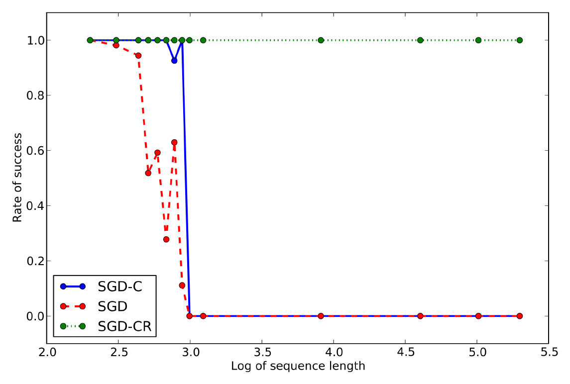
Figure 7 shows the success rate of standard SGD, SGD-C (SGD enhanced with out clipping strategy) and SGD-CR (SGD with the clipping strategy and the regularization term). Note that for sequences longer than 20, the vanishing gradients problem ensures that neither SGD nor SGD-C algorithms can solve the task. The $x$-axis is on log scale.
 {width=60%}
This task provides empirical evidence that exploding gradients are linked with tasks that require long memory traces. We know that initially the model operates in the one-attractor regime (i.e. $\lambda_{1}<1$), in which the amount of memory is controlled by $\lambda_{1}$. More memory means larger spectral radius, and, when this value crosses a certain threshold the model enters rich regimes where gradients are likely to explode. We see in Figure 7 that as long as the vanishing gradient problem does not become an issue, addressing the exploding gradients problem ensures a better success rate.
When combining clipping as well as the regularization term proposed in Section 3.3, we call this algorithm SGD-CR. SGD-CR solved the task with a success rate of 100% for sequences up to 200 steps (the maximal length used in [22]). Furthermore, we can train a single model to deal with any sequence of length 50 up to 200 (by providing sequences of different lengths for different SGD steps). Interestingly enough, the trained model can generalize to new sequences that can be twice as long as the ones seen during training.
4.1.2 Other pathological tasks
SGD-CR was also able to solve (100% success on the lengths listed below, for all but one task) other pathological problems proposed in [10], namely the addition problem, the multiplication problem, the 3-bit temporal order problem, the random permutation problem and the noiseless memorization problem in two variants (when the pattern needed to be memorized is 5 bits in length and when it contains over 20 bits of information; see [22]). For the first 4 problems we used a single model for lengths up to 200, while for the noiseless memorization we used a different model for each sequence length (50, 100, 150 and 200). The hardest problems for which only one trail out of 8 succeeded was the random permutation problem. In all cases, we observe successful generalization to sequences longer than the training sequences. In most cases, these results outperforms [22] in terms of success rate, they deal with longer sequences than in [10] and compared to [15] they generalize to longer sequences.
4.2 Natural problems
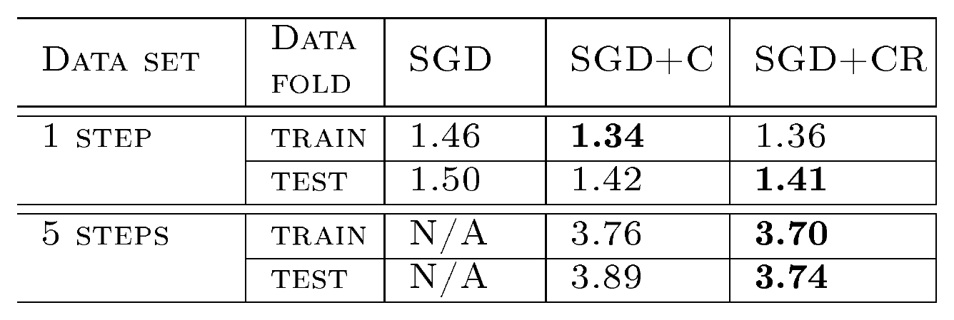
We address the task of polyphonic music prediction, using the datasets Piano-midi.de, Nottingham and MuseData described in [23] and language modelling at the character level on the Penn Treebank dataset ([24]). We also explore a modified version of the task, where we ask the model to predict the 5th character in the future (instead of the next). Our assumption is that to solve this modified task long term correlations are more important than short term ones, and hence our regularization term should be more helpful.
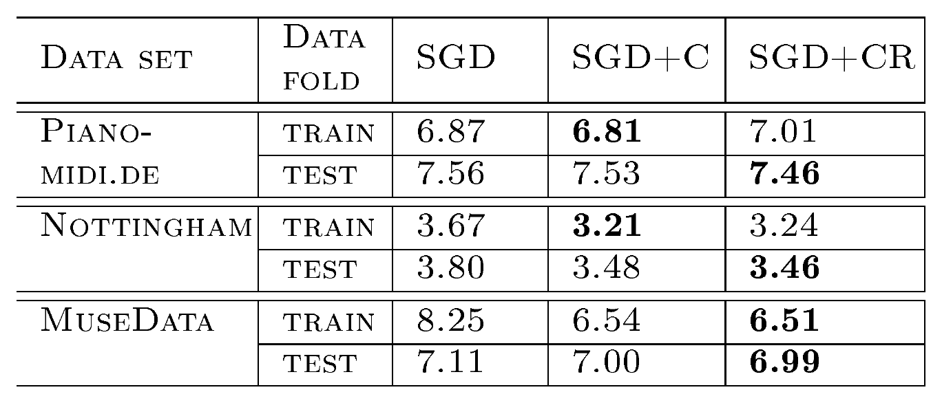
The training and test scores reported in Table 1 are average negative log likelihood per time step. We fixed hyper-parameters across the three runs, except for the regularization factor and clipping cutoff threshold. SGD-CR provides a statistically significant improvement on the state-of-the-art for RNNs on all the polyphonic music prediction tasks except for MuseData on which we get exactly the same performance as the state-of-the-art ([25]), which uses a different architecture. Table 2 contains the results on language modelling (in bits per letter).
::: {caption="Table 1: Results on polyphonic music prediction in negative log likelihood per time step. Lower is better."}
 {width=70%}
:::
::: {caption="Table 2: Results on the next character prediction task in entropy (bits/character)"}
 {width=70%}
:::
These results suggest that clipping the gradients solves an optimization issue and does not act as a regularizer, as both the training and test error improve in general. Results on Penn Treebank reach the state of the art achieved by [24], who used a different clipping algorithm similar to ours, thus providing evidence that both behave similarly. The regularized model performs as well as the Hessian-Free trained model.
By employing the proposed regularization term we are able to improve test error even on tasks that are not dominated by long term contributions.
5. Summary and Conclusions
Section Summary: The paper reviews the challenges of exploding and vanishing gradients in training recurrent networks and offers practical fixes for each. For exploding gradients, it introduces a simple clipping method that limits the size of the gradient when it grows too large, based on the idea that such explosions create steep valleys in the error surface. For vanishing gradients, it adds a regularization term that encourages the network to keep important error signals strong over time, and experiments show these steps improve results on both artificial test problems and real tasks such as music and language modeling.
We provided different perspectives through which one can gain more insight into the exploding and vanishing gradients issue. To deal with the exploding gradients problem, we propose a solution that involves clipping the norm of the exploded gradients when it is too large. The algorithm is motivated by the assumption that when gradients explode, the curvature and higher order derivatives explode as well, and we are faced with a specific pattern in the error surface, namely a valley with a single steep wall. In order to deal with the vanishing gradient problem we use a regularization term that forces the error signal not to vanish as it travels back in time. This regularization term forces the Jacobian matrices $\frac{\partial \mathbf{x}i}{\partial \mathbf{x}{i-1}}$ to preserve norm only in relevant directions. In practice we show that these solutions improve performance on both the pathological synthetic datasets considered as well as on polyphonic music prediction and language modelling.
Acknowledgements
We would like to thank the Theano development team as well (particularly to Frederic Bastien, Pascal Lamblin and James Bergstra) for their help.
We acknowledge NSERC, FQRNT, CIFAR, RQCHP and Compute Canada for the resources they provided.
6. Analytical analysis of the exploding and vanishing gradients problem
Section Summary: In recurrent networks the gradient of the loss at one time step with respect to an earlier hidden state is obtained by repeatedly multiplying by the transpose of the recurrent weight matrix, so its size is governed by the largest eigenvalue of that matrix raised to the length of the time gap. When the absolute value of this dominant eigenvalue exceeds one the product grows exponentially along the corresponding eigenvector direction, causing the overall parameter gradient to explode; when it is smaller than one the product shrinks toward zero and the gradient vanishes. The same spectral-radius condition therefore supplies a necessary criterion for stable training over long sequences.
$ \mathbf{x}{t} = \mathbf{W}{rec} \sigma(\mathbf{x}{t-1}) + \mathbf{W}{in} \mathbf{u}_{t} + \mathbf{b}\tag{2} $
Let us consider the term $\mathbf{g}_k^T=\frac{\partial \mathcal{E}_t}{\partial \mathbf{x}_t}\frac{\partial \mathbf{x}_t}{\partial \mathbf{x}_k} \frac{\partial^+ \mathbf{x}_k}{\partial \theta}$ for the linear version of the parametrization in equation 2 (i.e. set $\sigma$ to the identity function) and assume $t$ goes to infinity and $l=t-k$. We have that:
$ \frac{\partial \mathbf{x}_t}{\partial \mathbf{x}k} = \left(\mathbf{W}{rec}^{T}\right)^{l}\tag{11} $
By employing a generic power iteration method based proof we can show that, given certain conditions, $\frac{\partial \mathcal{E}_t}{\partial \mathbf{x}t}\left(\mathbf{W}{rec}^{T}\right)^{l}$ grows exponentially.
Proof: Let $\mathbf{W}_{rec}$ have the eigenvalues $\lambda_1, .., \lambda_n$ with $|\lambda_1| > |\lambda_2| > .. > |\lambda_n|$ and the corresponding eigenvectors $\mathbf{q}_1, \mathbf{q}_2, .., \mathbf{q}_n$ which form a vector basis. We can now write the row vector $\frac{\partial \mathcal{E}_t}{\partial \mathbf{x}_t}$ into this basis:
$\frac{\partial \mathcal{E}_t}{\partial \mathbf{x}t} = \sum{i=1}^N c_i \mathbf{q}i^T$ If $j$ is such that $c_j \neq 0$ and any $j'<j, c{j'}=0$, using the fact that $\mathbf{q}i^T \left(\mathbf{W}{rec}^T\right)^{l} = \lambda_i^{l} \mathbf{q}_i^T$ we have that
$ \frac{\partial \mathcal{E}_t}{\partial \mathbf{x}_t}\frac{\partial \mathbf{x}_t}{\partial \mathbf{x}_k} = c_j \lambda_j^{l} \mathbf{q}j^T + \lambda_j^{l}\sum{i={j+1}}^n c_i \frac{\lambda_i^l}{\lambda_j^l}\mathbf{q}_i^T \approx c_j \lambda_j^{l} \mathbf{q}_j^T\tag{12} $
We used the fact that $\left|\kern.1em^{\lambda_i}\kern-.3em/\kern-.1em_{\lambda_j}\right| <1$ for $i>j$, which means that $\lim_{l \to \infty} \left|\kern.1em^{\lambda_i}\kern-.3em/\kern-.1em_{\lambda_j}\right|^l = 0$. If $|\lambda_j| > 1$, it follows that $\frac{\partial \mathbf{x}_t}{\partial \mathbf{x}_k}$ grows exponentially fast with $l$, and it does so along the direction $\mathbf{q}_j$. $\Box$
The proof assumes $\mathbf{W}{rec}$ is diagonalizable for simplicity, though using the Jordan normal form of $\mathbf{W}{rec}$ one can extend this proof by considering not just the eigenvector of largest eigenvalue but the whole subspace spanned by the eigenvectors sharing the same (largest) eigenvalue.
This result provides a necessary condition for gradients to grow, namely that the spectral radius (the absolute value of the largest eigenvalue) of $\mathbf{W}_{rec}$ must be larger than 1.
If $\mathbf{q}_j$ is not in the null space of $\frac{\partial^+ \mathbf{x}_k}{\partial \theta}$ the entire temporal component grows exponentially with $l$. This approach extends easily to the entire gradient. If we re-write it in terms of the eigen-decomposition of $\mathbf{W}$, we get:
$ \frac{\partial \mathcal{E}t}{\partial \theta} = \sum{j=1}^n \left(\sum_{i=k}^t c_j \lambda_j^{t-k} \mathbf{q}_j^T \frac{\partial^{+} \mathbf{x}_k}{\partial \theta}\right)\tag{13} $
We can now pick $j$ and $k$ such that $c_j\mathbf{q}_j^T \frac{\partial^+ \mathbf{x}_k}{\partial \theta}$ does not have 0 norm, while maximizing $|\lambda_j|$. If for the chosen $j$ it holds that $|\lambda_j| > 1$ then $\lambda_j^{t-k} c_j \mathbf{q}_j^T \frac{\partial^+ \mathbf{x}_k}{\partial \theta}$ will dominate the sum and because this term grows exponentially fast to infinity with $t$, the same will happen to the sum.
7. Experimental setup
Section Summary: Hyper-parameters for all experiments were chosen via grid search on a validation set. The synthetic tasks used recurrent networks with 50–100 hidden units, specific learning rates, L2 regularization, and gradient clipping; models were trained on sequences of length 50–200 and evaluated by whether they achieved at most 1 % error on large test batches, with most tasks reaching 100 % success and generalizing to length-400 sequences. Similar training protocols, including sigmoid units and scheduled learning rates, were applied to the polyphonic music prediction benchmarks.
Note that all hyper-parameters where selected based on their performance on a validation set using a grid search.
The pathological synthetic tasks
Similar success criteria is used in all of the tasks below (borrowed from [22]), namely that the model should make no more than 1% error on a batch of 10000 test samples. In all cases, discrete symbols are depicted by a one-hot encoding, and in case of regression a prediction for a given sequence is considered as a success if the error is less than 0.04.
Addition problem
The input consists of a sequence of random numbers, where two random positions (one in the beginning and one in the middle of the sequence) are marked. The model needs to predict the sum of the two random numbers after the entire sequence was seen. For each generated sequence we sample the length $T'$ from $[T, \frac{11}{10}T]$, though for clarity we refer to $T$ as the length of the sequence in the paper. The first position is sampled from $[1, \frac{T'}{10}]$, while the second position is sampled from $[\frac{T'}{10}, \frac{T'}{2}]$. These positions $i, j$ are marked in a different input channel that is 0 everywhere except for the two sampled positions when it is 1. The model needs to predict the sum of the random numbers found at the sampled positions $i, j$ divided by 2.
To address this problem we use a 50 hidden units model, with a tanh activation function. The learning rate is set to .01 and the factor $\alpha$ in front of the regularization term is 0.5. We use clipping with a cut-off threshold of 6 on the norm of the gradients. The weights are initialized from a normal distribution with mean 0 and standard derivation $.1$.
The model is trained on sequences of varying length $T$ between 50 and 200. We manage to get a success rate of 100% at solving this task, which outperforms the results presented in [22] (using Hessian Free), where we see a decline in success rate as the length of the sequence gets closer to 200 steps. [10] only considers sequences up to 100 steps. [15] also addresses this task with 100% success rate, though the solution does not seem to generalize well as it relies on very large output weights, which for ESNs are usually a sign of instability. We use a single model to deal with all lengths of sequences (50, 100, 150 200), and the trained model generalizes to new sequences that can be up 400 steps (while the error is still under 1%).
Multiplication problem
This task is similar to the problem above, just that the predicted value is the product of the random numbers instead of the sum. We used the same hyper-parameters as for the previous case, and obtained very similar results.
Temporal order problem
For the temporal order the length of the sequence is fixed to $T$, We have a fixed set of two symbols ${A, B}$ and 4 distractor symbols ${c, d, e, f}$. The sequence entries are uniformly sampled from the distractor symbols everywhere except at two random positions, the first position sampled from $[\frac{T}{10}, \frac{2T}{10}]$, while the second from $[\frac{4T}{10}, \frac{5T}{10}]$. The task is to predict the order in which the non-distractor symbols were provided, i.e. either ${AA, AB, BA, BB}$.
We use a 50 hidden units model, with a learning rate of .001 and $\alpha$, the regularization coefficient, set to 2. The cut-off threshold for clipping the norm of the gradient is left to 6. As for the other two task we have a 100% success rate at training a single model to deal with sequences between 50 to 200 steps. This outperforms the previous state of the art because of the success rate, but also the single model generalizes to longer sequences (up to 400 steps).
3-bit temporal order problem
Similar to the previous one, except that we have 3 random positions, first sampled from $[\frac{T}{10}, \frac{2T}{10}]$, second from $[\frac{3T}{10}, \frac{4T}{10}]$ and last from $[\frac{6T}{10}, \frac{7T}{10}]$.
We use similar hyper-parameters as above, but that we increase the hidden layer size to 100 hidden units. As before we outperform the state of the art while training a single model that is able to generalize to new sequence lengths.
Random permutation problem
In this case we have a dictionary of 100 symbols. Except the first and last position which have the same value sampled from ${1, 2 }$ the other entries are randomly picked from $[3, 100]$. The task is to do next symbol prediction, though the only predictable symbol is the last one.
We use a 100 hidden units with a learning rate of .001 and $\alpha$, the regularization coefficient, set to 1. The cutoff threshold is left to 6. This task turns out to be more difficult to learn, and only 1 out of 8 experiments succeeded. As before we use a single model to deal with multiple values for $T$ (from 50 to 200 units).
Noiseless memorization problem
For the noiseless memorization we are presented with a binary pattern of length 5, followed by $T$ steps of constant value. After these $T$ steps the model needs to generate the pattern seen initially. We also consider the extension of this problem from [22], where the pattern has length 10, and the symbol set has cardinality 5 instead of 2.
We manage a 100% success rate on these tasks, though we train a different model for the 5 sequence lengths considered (50, 100, 150, 200).
Natural Tasks
Polyphonic music prediction
We train our model, a sigmoid units RNN, on sequences of 200 steps. The cut-off coefficient threshold is the same in all cases, namely 8 (note that one has to take the mean over the sequence length when computing the gradients).
In case of the Piano-midi.de dataset we use 300 hidden units and an initial learning rate of 1.0 (whir the learning rate halved every time the error over an epoch increased instead of decreasing). For the regularized model we used a initial value for regularization coefficient $\alpha$ of 0.5, where $\alpha$ follows a $1/t$ schedule, i.e. $\alpha_t = \frac{1}{2t}$ (where $t$ measures the number of epochs).
For the Nottingham dataset we used the exact same setup. For MuseData we increased the hidden layer to 400 hidden units. The learning rate was also decreased to 0.5. For the regularized model, the initial value for $\alpha$ was 0.1, and $\alpha_t = \frac{1}{t}$.
We make the observation that for natural tasks it seems useful to use a schedule that decreases the regularization term. We assume that the regularization term forces the model to focus on long term correlations at the expense of short term ones, so it may be useful to have this decaying factor in order to allow the model to make better use of the short term information.
Language modelling
For the language modelling task we used a 500 sigmoidal hidden units model with no biases ([24]). The model is trained over sequences of 200 steps, where the hidden state is carried over from one step to the next one.
We use a cut-off threshold of 45 (though we take the sum of the cost over the sequence length) for all experiments. For next character prediction we have a learning rate of 0.01 when using clipping with no regularization term, 0.05 when we add the regularization term and 0.001 when we do not use clipping. When predicting the 5th character in the future we use a learning rate of 0.05 with the regularization term and 0.1 without it.
The regularization factor $\alpha$ for next character prediction was set to .01 and kept constant, while for the modified task we used an initial value of 0.05 with a $\frac{1}{t}$ schedule.
References
Section Summary: This section compiles a list of 25 academic citations, mainly research papers, books, and technical reports on neural networks and machine learning. They span foundational studies from the 1980s and 1990s on training recurrent models, along with later work on optimization methods and sequence-related applications through 2012. The entries appear to support discussions of challenges like long-term dependency learning and practical improvements in network design.
[1] Bengio, Y., Simard, P., and Frasconi, P. (1994). Learning long-term dependencies with gradient descent is difficult. IEEE Transactions on Neural Networks, 5(2), 157–166.
[2] Rumelhart, D. E., Hinton, G. E., and Williams, R. J. (1986). Learning representations by back-propagating errors. Nature, 323(6088), 533–536.
[3] Elman, J. (1990). Finding structure in time. Cognitive Science, 14(2), 179–211.
[4] Werbos, P. J. (1988). Generalization of backpropagation with application to a recurrent gas market model. Neural Networks, 1(4), 339–356.
[5] Doya, K. (1993). Bifurcations of recurrent neural networks in gradient descent learning. IEEE Transactions on Neural Networks, 1, 75–80.
[6] Bengio, Y., Frasconi, P., and Simard, P. (1993). The problem of learning long-term dependencies in recurrent networks. pages 1183–1195, San Francisco. IEEE Press. (invited paper).
[7] Strogatz, S. (1994). Nonlinear Dynamics And Chaos: With Applications To Physics, Biology, Chemistry, And Engineering (Studies in Nonlinearity). Studies in nonlinearity. Perseus Books Group, 1 edition.
[8] Pascanu, R. and Jaeger, H. (2011). A neurodynamical model for working memory. Neural Netw., 24, 199–207.
[9] Doya, K. and Yoshizawa, S. (1991). Adaptive synchronization of neural and physical oscillators. In J. E. Moody, S. J. Hanson, and R. Lippmann, editors, NIPS, pages 109–116. Morgan Kaufmann.
[10] Hochreiter, S. and Schmidhuber, J. (1997). Long short-term memory. Neural Computation, 9(8), 1735–1780.
[11] Graves, A., Liwicki, M., Fernandez, S., Bertolami, R., Bunke, H., and Schmidhuber, J. (2009). A Novel Connectionist System for Unconstrained Handwriting Recognition. IEEE Transactions on Pattern Analysis and Machine Intelligence, 31(5), 855–868.
[12] Sutskever, I., Martens, J., and Hinton, G. (2011). Generating text with recurrent neural networks. In L. Getoor and T. Scheffer, editors, Proceedings of the 28th International Conference on Machine Learning (ICML-11), ICML '11, pages 1017–1024, New York, NY, USA. ACM.
[13] Lukoševičius, M. and Jaeger, H. (2009). Reservoir computing approaches to recurrent neural network training. Computer Science Review, 3(3), 127–149.
[14] Jaeger, H., Lukosevicius, M., Popovici, D., and Siewert, U. (2007). Optimization and applications of echo state networks with leaky- integrator neurons. Neural Networks, 20(3), 335–352.
[15] Jaeger, H. (2012). Long short-term memory in echo state networks: Details of a simulation study. Technical report, Jacobs University Bremen.
[16] Mikolov, T. (2012). Statistical Language Models based on Neural Networks. Ph.D. thesis, Brno University of Technology.
[17] Mikolov, T., Deoras, A., Kombrink, S., Burget, L., and Cernocky, J. (2011). Empirical evaluation and combination of advanced language modeling techniques. In Proc. 12th annual conference of the international speech communication association (INTERSPEECH 2011).
[18] Duchi, J. C., Hazan, E., and Singer, Y. (2011). Adaptive subgradient methods for online learning and stochastic optimization. Journal of Machine Learning Research, 12, 2121–2159.
[19] Moreira, M. and Fiesler, E. (1995). Neural networks with adaptive learning rate and momentum terms. Idiap-RR Idiap-RR-04-1995, IDIAP, Martigny, Switzerland.
[20] Bergstra, J., Breuleux, O., Bastien, F., Lamblin, P., Pascanu, R., Desjardins, G., Turian, J., Warde-Farley, D., and Bengio, Y. (2010). Theano: a CPU and GPU math expression compiler. In Proceedings of the Python for Scientific Computing Conference (SciPy). Oral Presentation.
[21] Bastien, F., Lamblin, P., Pascanu, R., Bergstra, J., Goodfellow, I., Bergeron, A., Bouchard, N., and Bengio, Y. (2012). Theano: new features and speed improvements. Submited to Deep Learning and Unsupervised Feature Learning NIPS 2012 Workshop.
[22] Martens, J. and Sutskever, I. (2011). Learning recurrent neural networks with Hessian-free optimization. In Proc. ICML'2011. ACM.
[23] Boulanger-Lewandowski, N., Bengio, Y., and Vincent, P. (2012). Modeling temporal dependencies in high-dimensional sequences: Application to polyphonic music generation and transcription. In Proceedings of the Twenty-nine International Conference on Machine Learning (ICML'12). ACM.
[24] Mikolov, T., Sutskever, I., Deoras, A., Le, H.-S., Kombrink, S., and Cernocky, J. (2012). Subword language modeling with neural networks. preprint (http://www.fit.vutbr.cz/ imikolov/rnnlm/char.pdf).
[25] Bengio, Y., Boulanger-Lewandowski, N., and Pascanu, R. (2012). Advances in optimizing recurrent networks. Technical Report arXiv:1212.0901, U. Montreal.