Pyramid Stereo Matching Network

Jia-Ren ChangYong-Sheng Chen

article2018CVPR1,843 citations

Introduces PSMNet, a stereo matching network that integrates spatial pyramid pooling and stacked 3D convolutional hourglass modules to exploit multi-scale global context and accurately estimate depth in challenging image regions.

Listen

Accurate depth estimation from stereo cameras is critical for real-world automated systems, including autonomous driving, 3D reconstruction, and object recognition. While deep learning methods have improved stereo matching, traditional architectures struggle in ill-posed visual regions—such as repetitive patterns, reflective surfaces, textureless areas, and occlusions—because they rely heavily on local pixel-level comparisons without sufficient global context.

The article aims to demonstrate that incorporating multiscale global context into a deep neural network enables accurate, end-to-end stereo depth estimation without requiring manual post-processing steps. To achieve this, the authors designed PSMNet, which combines a spatial pyramid pooling module to harvest hierarchical context with a stacked 3D convolutional hourglass network to regularize the matching volume.

The authors evaluated this approach on major standard benchmarks: the synthetic Scene Flow dataset (over 35,000 training pairs) and the real-world KITTI 2012 and 2015 autonomous driving benchmarks. The evaluation involved extensive ablation experiments to measure the impact of dilated convolutions, pooling scales, stacked architectures, and intermediate loss weighting schemes.

The key findings confirm that multiscale context significantly enhances stereo matching accuracy. PSMNet achieved rank-one standing on both the KITTI 2012 and KITTI 2015 public leaderboards as of March 2018. Specifically, on KITTI 2015, PSMNet achieved an overall three-pixel error rate of 2.32%, outperforming competing published methods. On KITTI 2012, it attained a three-pixel error rate of 1.89% across all areas and 1.49% in non-occluded regions. Furthermore, on the Scene Flow synthetic benchmark, PSMNet reached an end-point error of 1.09, outperforming previous baselines, while qualitative results showed marked improvements in challenging areas such as fences, car windows, and walls.

These findings indicate that end-to-end deep architectures can reliably resolve visual ambiguities in complex environments, eliminating the latency and tuning overhead of traditional post-processing pipelines. For safety-critical systems such as self-driving vehicles, higher depth accuracy in ill-posed regions reduces perception errors and lowers operational risk. However, there is a trade-off: PSMNet requires a runtime of approximately 0.41 seconds per image pair, which is slower than some lightweight alternatives that process frames in 0.12 to 0.22 seconds.

Organizations developing autonomous vision pipelines should consider adopting spatial pyramid pooling and 3D hourglass regularization when high accuracy is paramount. Where real-time deployment is required, future engineering efforts should focus on optimizing the 3D CNN module to reduce execution latency without sacrificing contextual reasoning.

Confidence in the reported accuracy is high due to rigorous validation against established public benchmarks and direct comparisons with state-of-the-art baselines. Users should note, however, that real-world performance depends on pre-training on synthetic data followed by domain-specific fine-tuning, and hardware constraints must accommodate the 0.41-second processing time.

National Chiao Tung University context information convolutional neural networks depth estimation Pyramid Stereo Matching Network spatial pyramid pooling disparity estimation

arXiv: 1803.08669 JiaRenChang/PSMNet

Paper: Pyramid Scene Parsing Network, Hengshuang Zhao et al. (2016). It introduces the spatial pyramid pooling module for multi-scale context aggregation that directly inspired the feature extraction design in PSMNet.
Paper: A Large Dataset to Train Convolutional Networks for Disparity, Optical Flow, and Scene Flow Estimation, Nikolaus Mayer et al. (2016). It provides the large-scale synthetic dataset (Scene Flow) and end-to-end convolutional matching foundations that PSMNet pre-trains on and builds upon.
Paper: Spatial Pyramid Pooling in Deep Convolutional Networks for Visual Recognition, Kaiming He et al. (2014). It establishes the foundational Spatial Pyramid Pooling (SPP) concept for capturing multi-scale contextual representations across varying receptive fields.
Paper: Convolutional Pose Machines, Shih-En Wei et al. (2016). It introduces multi-stage sequential prediction with intermediate supervision, which forms the core training strategy of PSMNet's stacked hourglass 3D CNN.
Paper: FlowNet: Learning Optical Flow with Convolutional Networks, Philipp Fischer et al. (2015). It pioneered end-to-end deep learning for visual correspondence and cost-volume correlation layers that modern learned stereo architectures rely on.

Paper: PWC-Net: CNNs for Optical Flow Using Pyramid, Warping, and Cost Volume, Deqing Sun et al. (2018). It adapts the principles of pyramid features and explicit cost volumes to design a highly compact, warp-based neural network for optical flow estimation.
Paper: SuperGlue: Learning Feature Matching With Graph Neural Networks, Paul-Edouard Sarlin et al. (2020). It advances beyond dense 3D CNN regularization of cost volumes by framing correspondence matching as graph-based context aggregation with optimal transport.
Paper: Vision Transformers for Dense Prediction, René Ranftl et al. (2021). It explores vision transformers as an alternative to spatial pyramid convolutions and 3D CNNs for global-context dense depth estimation.

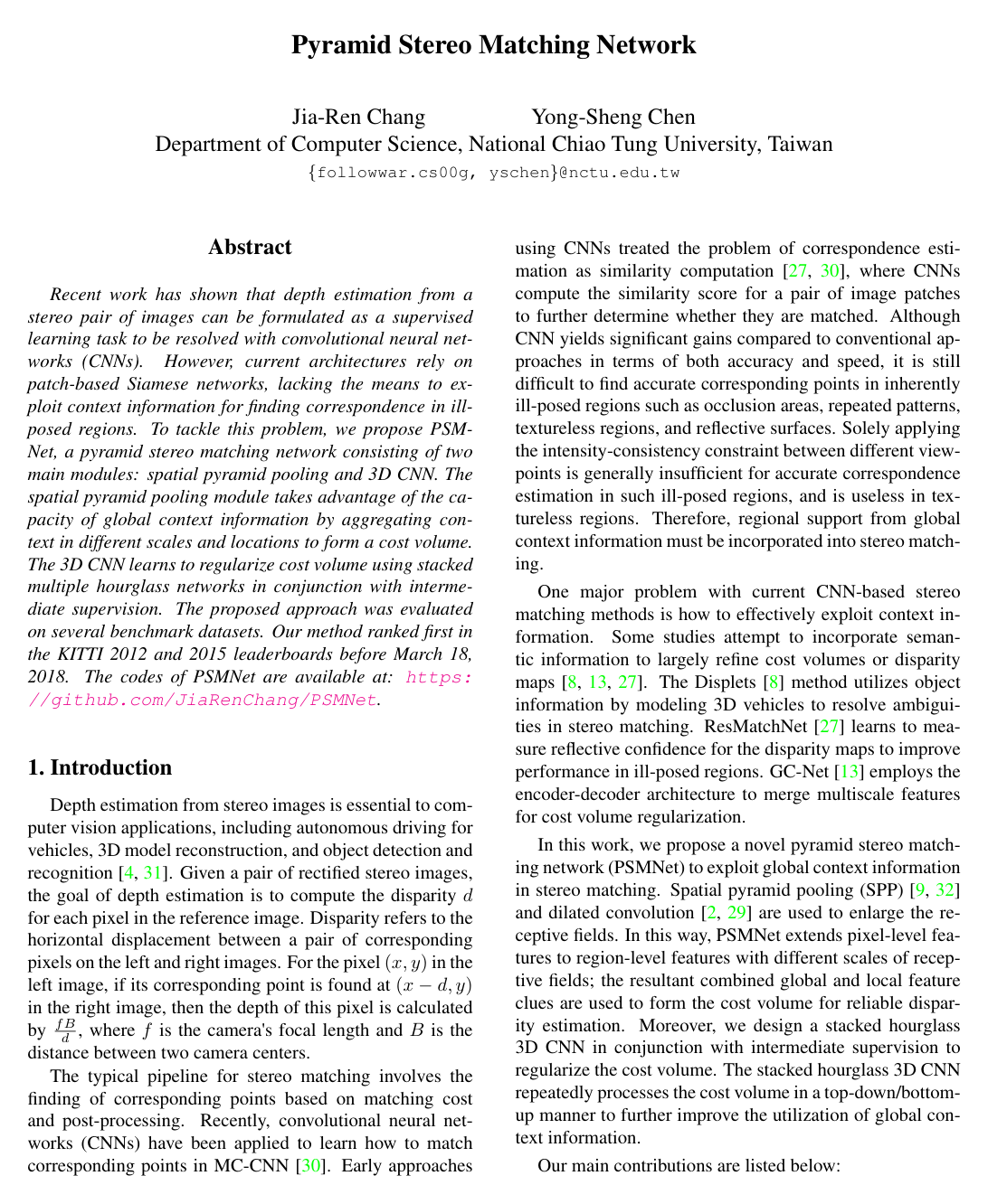
Cover for Pyramid Stereo Matching Network

Abstract

Recent work has shown that depth estimation from a stereo pair of images can be formulated as a supervised learning task to be resolved with convolutional neural networks (CNNs). However, current architectures rely on patch-based Siamese networks, lacking the means to exploit context information for finding correspondence in illposed regions. To tackle this problem, we propose PSMNet, a pyramid stereo matching network consisting of two main modules: spatial pyramid pooling and 3D CNN. The spatial pyramid pooling module takes advantage of the capacity of global context information by aggregating context in different scales and locations to form a cost volume. The 3D CNN learns to regularize cost volume using stacked multiple hourglass networks in conjunction with intermediate supervision. The proposed approach was evaluated on several benchmark datasets. Our method ranked first in the KITTI 2012 and 2015 leaderboards before March 18, 2018. The codes of PSMNet are available at: this https URL.

1 Introduction
2 Related Work
3 Pyramid Stereo Matching Network
3.1 Network Architecture
3.2 Spatial Pyramid Pooling Module
3.3 Cost Volume
3.4 3D CNN
3.5 Disparity Regression
3.6 Loss
4 Experiments
4.1 Experiment Details
4.2 KITTI 2015
4.3 Scene Flow
4.4 KITTI 2012
5 Conclusions
References

Knowls

Knowl 1 — PSMNet End-to-End Stereo Matching Framework
model/method
The Pyramid Stereo Matching Network (PSMNet) is an end-to-end convolutional neural network for disparity estimation from rectified stereo image pairs without any post-processing steps (such as semi-global matching or disparity refinement filters).

Given a rectified stereo pair consisting of a left reference image $I_L$ and a right image $I_R$ of size $H \times W \times 3$ , PSMNet operates via the following pipeline:
1. Unary Feature Extraction: Weight-sharing 2D CNN backbones process $I_L$ and $I_R$ . The early layers cascade three $3 \times 3$ convolutions (replacing a single $7 \times 7$ filter) followed by residual blocks (conv1_x through conv4_x). Subsampling by stride-2 convolutions at conv0_1 and conv2_1 reduces the spatial resolution to $\frac{1}{4}H \times \frac{1}{4}W$ . Dilated convolutions with dilation rates of 2 and 4 are applied in conv3_x and conv4_x to expand the receptive field.
2. Spatial Pyramid Pooling (SPP): An SPP module collects contextual information at four spatial scales ( $64 \times 64$ , $32 \times 32$ , $16 \times 16$ , $8 \times 8$ ) using adaptive average pooling, followed by $1 \times 1$ convolutions and bilinear upsampling. The pooled features are concatenated with intermediate features and fused into a 32-channel feature map per image.
3. 4D Cost Volume Construction: A 4D cost volume of shape $\frac{1}{4}D_{\max} \times \frac{1}{4}H \times \frac{1}{4}W \times 64$ is formed by concatenating the 32-channel left feature map with the corresponding right feature map shifted horizontally by disparity candidate $d \in \{0, 1, \dots, \frac{1}{4}D_{\max}-1\}$ .
4. 3D CNN Cost Volume Regularization: A 3D CNN (either a basic 12-layer 3D CNN or a stacked hourglass 3D CNN with three encoder-decoder blocks) regularizes the cost volume by aggregating spatial and disparity context across multiple scales.
5. Disparity Regression: The regularized 4D volume is bilinearly upsampled to full resolution $D_{\max} \times H \times W$ . A differentiable softmax operation across the disparity dimension produces a probability distribution, and disparity regression computes the final continuous disparity map of size $H \times W$ .
Knowl 2 — Spatial Pyramid Pooling Module for Stereo Matching
model/method
The Spatial Pyramid Pooling (SPP) module in PSMNet aggregates global and multiscale context to incorporate object-level relationships into pixel-level representations, aiding correspondence estimation in ambiguous, textureless, reflective, and occluded regions.

The SPP module processes feature representations from the unary feature extraction backbone at $\frac{1}{4}H \times \frac{1}{4}W$ resolution. It consists of four fixed-size average pooling branches:
- Branch 1: $64 \times 64$ average pooling
- Branch 2: $32 \times 32$ average pooling
- Branch 3: $16 \times 16$ average pooling
- Branch 4: $8 \times 8$ average pooling
Each pooling branch is followed by a $3 \times 3$ convolution reducing the channel dimension to 32, after which bilinear interpolation upsamples the feature maps back to $\frac{1}{4}H \times \frac{1}{4}W$ .

The module concatenates six feature tensors along the channel dimension:
1. The 64-channel feature map from conv2_16
2. The 128-channel feature map from conv4_3 (with dilation rate 4)
3. The four 32-channel upsampled branch feature maps ( $4 \times 32 = 128$ channels)
This yields a concatenated tensor with 320 channels ( $64 + 128 + 128 = 320$ ). A fusion block consisting of a $3 \times 3$ convolution (128 channels) followed by a $1 \times 1$ convolution (32 channels) produces the final 32-channel feature map used for cost volume construction.
Knowl 3 — Stacked Hourglass 3D CNN for Cost Volume Regularization
model/method
The stacked hourglass 3D CNN in PSMNet regularizes the 4D matching cost volume by repeatedly applying top-down and bottom-up encoder-decoder processing to aggregate context along both the disparity dimension and spatial dimensions.

The input 4D cost volume of size $\frac{1}{4}D_{\max} \times \frac{1}{4}H \times \frac{1}{4}W \times 64$ is first processed by two preliminary 3D convolutional blocks (3Dconv0 and 3Dconv1, each containing two $3 \times 3 \times 3$ convs with 32 channels).

The architecture then stacks three 3D hourglass sub-networks:
- Encoder: Each hourglass downsamples the volume twice by a factor of 2 across spatial and disparity dimensions using stride-2 $3 \times 3 \times 3$ convolutions: first to $\frac{1}{8}D_{\max} \times \frac{1}{8}H \times \frac{1}{8}W \times 64$ , and then to $\frac{1}{16}D_{\max} \times \frac{1}{16}H \times \frac{1}{16}W \times 64$ .
- Decoder: Resolution is restored using $3 \times 3 \times 3$ 3D transposed convolutions (deconvolutions) with stride 2. Skip connections add encoder features from corresponding scales (3Dstack1_1 and 3Dconv1) to the upsampled features. Subsequent hourglass modules also incorporate skip connections from the previous hourglass decoders (3Dstack1_3 and 3Dstack2_3).
- Intermediate Outputs: Each of the three hourglass modules branches into two $3 \times 3 \times 3$ convolutions to generate a 1-channel 4D volume of size $\frac{1}{4}D_{\max} \times \frac{1}{4}H \times \frac{1}{4}W \times 1$ (output_1, output_2, output_3). In the second and third modules, the output of the preceding stage is added prior to final regression (output_2 = 3Dconv + output_1, output_3 = 3Dconv + output_2).
Each of the three intermediate volumes is bilinearly upsampled to $D_{\max} \times H \times W$ and passed to disparity regression, generating three disparity predictions for intermediate supervision during training. At test time, only the final disparity map generated from output_3 is used.
Knowl 4 — Disparity Regression via Differentiable Soft Argmin
equation
Disparity regression estimates continuous sub-pixel disparity values directly from the matching costs predicted by the 3D regularization network. For each pixel, the predicted continuous disparity $\hat{d}$ is computed as the expected value across all candidate disparities:

$\hat{d} = \sum_{d=0}^{D_{\max}} d \times \sigma(-c_d) = \sum_{d=0}^{D_{\max}} d \times \frac{\exp(-c_d)}{\sum_{d'=0}^{D_{\max}} \exp(-c_{d'})}$

where:
- $d \in \{0, 1, 2, \dots, D_{\max}\}$ denotes the candidate disparity value.
- $D_{\max}$ is the predefined maximum disparity search range.
- $c_d \in \mathbb{R}$ is the regularized cost predicted by the 3D CNN for disparity level $d$ at a given pixel.
- $\sigma(-c_d) \in [0, 1]$ is the normalized probability of disparity $d$ obtained via the softmax operator over the negated cost volume values along the disparity axis, ensuring $\sum_{d=0}^{D_{\max}} \sigma(-c_d) = 1$ .
This formulation acts as a soft attention mechanism that is fully differentiable, allowing end-to-end training and avoiding quantization errors associated with discrete classification.
Knowl 5 — Smooth L1 Loss with Intermediate Supervision
equation
PSMNet is trained using the smooth $L_1$ loss function, which provides robustness and low sensitivity to disparity outliers compared to $L_2$ loss. The loss for a disparity map prediction is defined as:

$L(d, \hat{d}) = \frac{1}{N} \sum_{i=1}^N \text{smooth}_{L_1}(d_i - \hat{d}_i)$

where $N$ is the number of labeled ground-truth pixels, $d_i$ is the ground-truth disparity at pixel $i$ , $\hat{d}_i$ is the predicted disparity at pixel $i$ , and:

$\text{smooth}_{L_1}(x) = \begin{cases} 0.5 x^2, & \text{if } |x| < 1 \\ |x| - 0.5, & \text{otherwise} \end{cases}$

When training the stacked hourglass 3D CNN architecture, intermediate supervision is applied across all three hourglass outputs using a weighted sum of losses:

$L_{\text{total}} = w_1 L_1(d, \hat{d}^{(1)}) + w_2 L_2(d, \hat{d}^{(2)}) + w_3 L_3(d, \hat{d}^{(3)})$

where $\hat{d}^{(1)}, \hat{d}^{(2)}, \hat{d}^{(3)}$ are the disparity maps computed from output_1, output_2, and output_3 respectively. The empirical optimal loss weights are $w_1 = 0.5$ , $w_2 = 0.7$ , and $w_3 = 1.0$ .

Knowl 6 — PSMNet Layer-by-Layer Architectural Specifications

data/table

The complete layer parameters, kernel sizes, channels, residual blocks, strides, dilation rates, and output dimensions of PSMNet are detailed in the table below. Here $H$ and $W$ denote the height and width of the input stereo image, and $D$ denotes the maximum disparity setting.

Name	Layer setting	Output dimension
input	-	$H \times W \times 3$
CNN Backbone
conv0_1	$3 \times 3, 32$ , stride 2	$\frac{1}{2}H \times \frac{1}{2}W \times 32$
conv0_2	$3 \times 3, 32$	$\frac{1}{2}H \times \frac{1}{2}W \times 32$
conv0_3	$3 \times 3, 32$	$\frac{1}{2}H \times \frac{1}{2}W \times 32$
conv1_x	$[3 \times 3, 32; 3 \times 3, 32] \times 3$	$\frac{1}{2}H \times \frac{1}{2}W \times 32$
conv2_x	$[3 \times 3, 64; 3 \times 3, 64] \times 16$ , stride 2	$\frac{1}{4}H \times \frac{1}{4}W \times 64$
conv3_x	$[3 \times 3, 128; 3 \times 3, 128] \times 3$ , dila = 2	$\frac{1}{4}H \times \frac{1}{4}W \times 128$
conv4_x	$[3 \times 3, 128; 3 \times 3, 128] \times 3$ , dila = 4	$\frac{1}{4}H \times \frac{1}{4}W \times 128$
SPP Module
branch_1	$64 \times 64$ avg. pool, $3 \times 3, 32$ , bilinear interp.	$\frac{1}{4}H \times \frac{1}{4}W \times 32$
branch_2	$32 \times 32$ avg. pool, $3 \times 3, 32$ , bilinear interp.	$\frac{1}{4}H \times \frac{1}{4}W \times 32$
branch_3	$16 \times 16$ avg. pool, $3 \times 3, 32$ , bilinear interp.	$\frac{1}{4}H \times \frac{1}{4}W \times 32$
branch_4	$8 \times 8$ avg. pool, $3 \times 3, 32$ , bilinear interp.	$\frac{1}{4}H \times \frac{1}{4}W \times 32$
concat	Concat[conv2_16, conv4_3, branch_1, branch_2, branch_3, branch_4]	$\frac{1}{4}H \times \frac{1}{4}W \times 320$
fusion	$3 \times 3, 128 \to 1 \times 1, 32$	$\frac{1}{4}H \times \frac{1}{4}W \times 32$
Cost Volume
Cost volume	Concat left and shifted right features	$\frac{1}{4}D \times \frac{1}{4}H \times \frac{1}{4}W \times 64$
3D CNN (Stacked Hourglass)
3Dconv0	$3 \times 3 \times 3, 32; 3 \times 3 \times 3, 32$	$\frac{1}{4}D \times \frac{1}{4}H \times \frac{1}{4}W \times 32$
3Dconv1	$3 \times 3 \times 3, 32; 3 \times 3 \times 3, 32$	$\frac{1}{4}D \times \frac{1}{4}H \times \frac{1}{4}W \times 32$
3Dstack1_1	$3 \times 3 \times 3, 64; 3 \times 3 \times 3, 64$ , stride 2	$\frac{1}{8}D \times \frac{1}{8}H \times \frac{1}{8}W \times 64$
3Dstack1_2	$3 \times 3 \times 3, 64; 3 \times 3 \times 3, 64$ , stride 2	$\frac{1}{16}D \times \frac{1}{16}H \times \frac{1}{16}W \times 64$
3Dstack1_3	deconv $3 \times 3 \times 3, 64$ , stride 2; add 3Dstack1_1	$\frac{1}{8}D \times \frac{1}{8}H \times \frac{1}{8}W \times 64$
3Dstack1_4	deconv $3 \times 3 \times 3, 32$ , stride 2; add 3Dconv1	$\frac{1}{4}D \times \frac{1}{4}H \times \frac{1}{4}W \times 32$
3Dstack2_1	$3 \times 3 \times 3, 64; 3 \times 3 \times 3, 64$ , stride 2; add 3Dstack1_3	$\frac{1}{8}D \times \frac{1}{8}H \times \frac{1}{8}W \times 64$
3Dstack2_2	$3 \times 3 \times 3, 64; 3 \times 3 \times 3, 64$ , stride 2	$\frac{1}{16}D \times \frac{1}{16}H \times \frac{1}{16}W \times 64$
3Dstack2_3	deconv $3 \times 3 \times 3, 64$ , stride 2; add 3Dstack1_1	$\frac{1}{8}D \times \frac{1}{8}H \times \frac{1}{8}W \times 64$
3Dstack2_4	deconv $3 \times 3 \times 3, 32$ , stride 2; add 3Dconv1	$\frac{1}{4}D \times \frac{1}{4}H \times \frac{1}{4}W \times 32$
3Dstack3_1	$3 \times 3 \times 3, 64; 3 \times 3 \times 3, 64$ , stride 2; add 3Dstack2_3	$\frac{1}{8}D \times \frac{1}{8}H \times \frac{1}{8}W \times 64$
3Dstack3_2	$3 \times 3 \times 3, 64; 3 \times 3 \times 3, 64$ , stride 2	$\frac{1}{16}D \times \frac{1}{16}H \times \frac{1}{16}W \times 64$
3Dstack3_3	deconv $3 \times 3 \times 3, 64$ , stride 2; add 3Dstack1_1	$\frac{1}{8}D \times \frac{1}{8}H \times \frac{1}{8}W \times 64$
3Dstack3_4	deconv $3 \times 3 \times 3, 32$ , stride 2; add 3Dconv1	$\frac{1}{4}D \times \frac{1}{4}H \times \frac{1}{4}W \times 32$
output_1	$3 \times 3 \times 3, 32; 3 \times 3 \times 3, 1$	$\frac{1}{4}D \times \frac{1}{4}H \times \frac{1}{4}W \times 1$
output_2	$3 \times 3 \times 3, 32; 3 \times 3 \times 3, 1$ ; add output_1	$\frac{1}{4}D \times \frac{1}{4}H \times \frac{1}{4}W \times 1$
output_3	$3 \times 3 \times 3, 32; 3 \times 3 \times 3, 1$ ; add output_2	$\frac{1}{4}D \times \frac{1}{4}H \times \frac{1}{4}W \times 1$
Output Stage
upsampling	Bilinear interpolation	$D \times H \times W$
Disparity Reg.	Softmax + Disparity Regression	$H \times W$

Batch normalization and ReLU activations follow ResNet conventions, except that ReLU is not applied after tensor summations.

Knowl 7 — Dataset Protocols and Training Setup
experimental setup
PSMNet was evaluated on three stereo benchmarks under the following protocols:
1. Scene Flow: A synthetic dataset containing 35,454 training and 4,370 testing stereo pairs ( $H = 540, W = 960$ ) with dense ground-truth disparity maps. Disparities exceeding the maximum search range are excluded from loss computation.
2. KITTI 2015: A real-world dataset of 200 training stereo pairs with sparse LiDAR ground-truth disparities ( $H = 376, W = 1240$ ) and 200 testing pairs. For experimental validation, the training data is split into a training set (80%, 160 image pairs) and a validation set (20%, 40 image pairs).
3. KITTI 2012: A real-world dataset of 194 training stereo pairs with sparse LiDAR ground-truth disparities ( $H = 376, W = 1240$ ) and 195 testing pairs. The training data is split into 160 training pairs and 34 validation pairs.
Training Implementation Details:
- Framework & Optimizer: Implemented in PyTorch and optimized end-to-end using Adam ( $\beta_1 = 0.9, \beta_2 = 0.999$ ).
- Preprocessing: Color normalization is applied across all input images. Training crops are randomly sampled at size $H = 256, W = 512$ . The maximum disparity $D$ is set to 192.
- Pretraining: Models are trained from scratch on Scene Flow for 10 epochs at a constant learning rate of 0.001 with batch size 12 across four Nvidia Titan-Xp GPUs (~13 hours).
- Fine-tuning: For KITTI, the Scene Flow pretrained weights are fine-tuned on the KITTI training sets for 300 epochs (learning rate 0.001 for epochs 1–200, reduced to 0.0001 for epochs 201–300; ~5 hours). Training is extended to 1000 epochs to produce final models for benchmark submission.

Knowl 8 — Ablation Study on Receptive Field and Context Architecture

data/table

An ablation study evaluated the relative contributions of dilated convolution, multiscale pyramid pooling levels, and 3D CNN regularization structures. Error was measured by the percentage of three-pixel-error on the KITTI 2015 validation set and End-Point Error (EPE in pixels) on the Scene Flow test set.

Dilated Conv	Pyramid Pooling Size				Stacked Hourglass	KITTI 2015	Scene Flow
Dilated Conv	$64 \times 64$	$32 \times 32$	$16 \times 16$	$8 \times 8$	Stacked Hourglass	Val Err (%)	End Point Err (px)
						2.43	1.43
✓						2.16	1.56
	✓	✓	✓	✓		2.47	1.40
✓	✓	✓				2.17	1.30
✓	✓	✓	✓	✓		2.09	1.28
✓	✓	✓	✓	✓	✓	1.98	1.09
$✓^*$ $	✓	✓	✓	✓	✓	1.83	1.12

*Note: $\checkmark^*$ indicates using half the dilation rate (rates of 1 and 2 instead of 2 and 4).

The results demonstrate that:

Dilated convolutions alone reduce KITTI validation error from 2.43% to 2.16% by enlarging the receptive field.
Pyramid pooling combined with dilated convolution progressively improves accuracy as more pooling scales are added (2.09% validation error with 4 scales vs. 2.17% with 2 scales).
Replacing the 12-layer basic 3D CNN with the stacked hourglass 3D CNN drops the KITTI 2015 validation error from 2.09% to 1.98% and Scene Flow EPE from 1.28 px to 1.09 px.
Halving the dilation rate in conjunction with the full SPP and stacked hourglass modules achieves the best KITTI 2015 validation error of 1.83%.

Knowl 9 — Ablation Study on Intermediate Supervision Loss Weights

data/table

An ablation study evaluated the influence of different weighting schemes $(w_1, w_2, w_3)$ for the three intermediate losses (Loss_1, Loss_2, Loss_3) generated by the three stages of the stacked hourglass 3D CNN on the KITTI 2015 validation set.

Loss Weight			KITTI 2015
$\text{Loss\_1}$	$\text{Loss\_2}$	$\text{Loss\_3}$	Val Error (%)
0.0	0.0	1.0	2.49
0.1	0.3	1.0	2.07
0.3	0.5	1.0	2.05
0.5	0.7	1.0	1.98
0.7	0.9	1.0	2.05
1.0	1.0	1.0	2.01

Training without intermediate supervision ( $w_1 = 0.0, w_2 = 0.0, w_3 = 1.0$ ) resulted in a validation error of 2.49%. Introducing progressively increasing weights across the stages ( $0.5, 0.7, 1.0$ ) provided the lowest validation error of 1.98%, outperforming equal weighting ( $1.0, 1.0, 1.0$ , which achieved 2.01%).

Knowl 10 — Benchmark Results on KITTI 2012, KITTI 2015, and Scene Flow

data/table

PSMNet was evaluated on the official test evaluation servers of KITTI 2015 and KITTI 2012, as well as on the Scene Flow test set.

KITTI 2015 Leaderboard (Test Set)

The benchmark measures the percentage of pixels with disparity error $> 3\text{ px}$ or $> 5\%$ of true disparity for background (D1-bg), foreground (D1-fg), and all (D1-all) areas, across all pixels (All) and non-occluded pixels (Noc):

Rank	Method	All (%)			Noc (%)			Runtime (s)
Rank	Method	D1-bg	D1-fg	D1-all	D1-bg	D1-fg	D1-all	Runtime (s)
1	PSMNet (ours)	1.86	4.62	2.32	1.71	4.31	2.14	0.41
3	iResNet-i2e2	2.14	3.45	2.36	1.94	3.20	2.15	0.22
6	iResNet	2.35	3.23	2.50	2.15	2.55	2.22	0.12
8	CRL	2.48	3.59	2.67	2.32	3.12	2.45	0.47
11	GC-Net	2.21	6.16	2.87	2.02	5.58	2.61	0.90

KITTI 2012 Leaderboard (Test Set)

The benchmark measures error percentage for threshold cutoffs of $>2\text{ px}$ , $>3\text{ px}$ , and $>5\text{ px}$ , as well as mean disparity error in pixels:

Rank	Method	$>$ 2 px		$>$ 3 px		$>$ 5 px		Mean Error (px)		Runtime (s)
Rank	Method	Noc	All	Noc	All	Noc	All	Noc	All	Runtime (s)
1	PSMNet (ours)	2.44	3.01	1.49	1.89	0.90	1.15	0.5	0.6	0.41
2	iResNet-i2	2.69	3.34	1.71	2.16	1.06	1.32	0.5	0.6	0.12
4	GC-Net	2.71	3.46	1.77	2.30	1.12	1.46	0.6	0.7	0.90
11	L-ResMatch	3.64	5.06	2.27	3.40	1.50	2.26	0.7	1.0	48
14	SGM-Net	3.60	5.15	2.29	3.50	1.60	2.36	0.7	0.9	67

Scene Flow Test Set Comparison

End-Point Error (EPE in pixels) across all tested methods:

PSMNet achieved the top ranking on both the KITTI 2012 and KITTI 2015 public leaderboards prior to March 18, 2018.

Coverage note — All core architectural components, mathematical formulations, training strategies, ablation experiments, and benchmark evaluations were extracted into self-contained knowls; no substantial contributed material was omitted.

References

1.D. Bahdanau, K. Cho, and Y. Bengio. Neural machine translation by jointly learning to align and translate. In ICLR, 2015. 5
2.L.-C. Chen, G. Papandreou, I. Kokkinos, K. Murphy, and A. L. Yuille. DeepLab: Semantic image segmentation with deep convolutional nets, atrous convolution, and fully connected crfs. arXiv preprint arXiv:1606.00915, 2016. 1, 2
3.L.-C. Chen, G. Papandreou, F. Schroff, and H. Adam. Rethinking atrous convolution for semantic image segmentation. arXiv preprint arXiv:1706.05587, 2017. 2
4.X. Chen, K. Kundu, Y. Zhu, A. G. Berneshawi, H. Ma, S. Fidler, and R. Urtasun. 3D object proposals for accurate object class detection. In Advances in Neural Information Processing Systems, pages 424–432, 2015. 1
5.J. Fu, J. Liu, Y. Wang, and H. Lu. Stacked deconvolutional network for semantic segmentation. arXiv preprint arXiv:1708.04943, 2017. 2
6.S. Gidaris and N. Komodakis. Detect, replace, refine: Deep structured prediction for pixel wise labeling. In The IEEE Conference on Computer Vision and Pattern Recognition (CVPR), July 2017. 2
7.R. Girshick. Fast R-CNN. In Proceedings of the IEEE international conference on computer vision, pages 1440–1448, 2015. 5
8.F. Guney and A. Geiger. Displets: Resolving stereo ambiguities using object knowledge. In Proceedings of the IEEE Conference on Computer Vision and Pattern Recognition, pages 4165–4175, 2015. 1, 2
9.K. He, X. Zhang, S. Ren, and J. Sun. Spatial pyramid pooling in deep convolutional networks for visual recognition. In European Conference on Computer Vision, pages 346–361. Springer, 2014. 1, 3
10.K. He, X. Zhang, S. Ren, and J. Sun. Deep residual learning for image recognition. In Proceedings of the IEEE conference on computer vision and pattern recognition, pages 770–778, 2016. 3, 5
11.H. Hirschmuller. Accurate and efficient stereo processing by semi-global matching and mutual information. In Computer Vision and Pattern Recognition, 2005. CVPR 2005. IEEE Computer Society Conference on, volume 2, pages 807–814. IEEE, 2005. 2
12.M. A. Islam, S. Naha, M. Rochan, N. Bruce, and Y. Wang. Label refinement network for coarse-to-fine semantic segmentation. arXiv preprint arXiv:1703.00551, 2017. 2
13.A. Kendall, H. Martirosyan, S. Dasgupta, P. Henry, R. Kennedy, A. Bachrach, and A. Bry. End-to-end learning of geometry and context for deep stereo regression. In The IEEE International Conference on Computer Vision (ICCV), Oct 2017. 1, 2, 4, 5, 6, 7, 8
14.Z. Liang, Y. Feng, Y. Guo, H. Liu, L. Qiao, W. Chen, L. Zhou, and J. Zhang. Learning deep correspondence through prior and posterior feature constancy. arXiv preprint arXiv:1712.01039, 2017. 7, 8
15.G. Lin, A. Milan, C. Shen, and I. Reid. RefineNet: Multi-path refinement networks for high-resolution semantic segmentation. In The IEEE Conference on Computer Vision and Pattern Recognition (CVPR), July 2017. 2
16.W. Liu, A. Rabinovich, and A. C. Berg. ParseNet: Looking wider to see better. arXiv preprint arXiv:1506.04579, 2015. 2, 3
17.J. Long, E. Shelhamer, and T. Darrell. Fully convolutional networks for semantic segmentation. In Proceedings of the IEEE Conference on Computer Vision and Pattern Recognition, pages 3431–3440, 2015. 2
18.W. Luo, A. G. Schwing, and R. Urtasun. Efficient deep learning for stereo matching. In Proceedings of the IEEE Conference on Computer Vision and Pattern Recognition, pages 5695–5703, 2016. 2
19.N. Mayer, E. Ilg, P. Hausser, P. Fischer, D. Cremers, A. Dosovitskiy, and T. Brox. A large dataset to train convolutional networks for disparity, optical flow, and scene flow estimation. In The IEEE Conference on Computer Vision and Pattern Recognition (CVPR), June 2016. 2, 6, 7
20.A. Newell, K. Yang, and J. Deng. Stacked hourglass networks for human pose estimation. In European Conference on Computer Vision, pages 483–499. Springer, 2016. 2
21.J. Pang, W. Sun, J. S. Ren, C. Yang, and Q. Yan. Cascade residual learning: A two-stage convolutional neural network for stereo matching. In The IEEE International Conference on Computer Vision (ICCV), Oct 2017. 2, 6, 7
22.P. O. Pinheiro, T.-Y. Lin, R. Collobert, and P. Doll%r. Learning to refine object segments. In European Conference on Computer Vision, pages 75–91. Springer, 2016. 2
23.A. Ranjan and M. J. Black. Optical flow estimation using a spatial pyramid network. In IEEE Conference on Computer Vision and Pattern Recognition (CVPR), volume 2, 2017. 2
24.O. Ronneberger, P. Fischer, and T. Brox. U-Net: Convolutional networks for biomedical image segmentation. In International Conference on Medical Image Computing and Computer-Assisted Intervention, pages 234–241. Springer, 2015. 2
25.D. Scharstein and R. Szeliski. A taxonomy and evaluation of dense two-frame stereo correspondence algorithms. International journal of computer vision, 47(1-3):7–42, 2002. 2
26.A. Seki and M. Pollefeys. SGM-Nets: Semi-global matching with neural networks. In The IEEE Conference on Computer Vision and Pattern Recognition (CVPR), July 2017. 2, 8
27.A. Shaked and L. Wolf. Improved stereo matching with constant highway networks and reflective confidence learning. In The IEEE Conference on Computer Vision and Pattern Recognition (CVPR), July 2017. 1, 2, 8
28.D. Sun, X. Yang, M.-Y. Liu, and J. Kautz. PWC-Net: CNNs for optical flow using pyramid, warping, and cost volume. arXiv preprint arXiv:1709.02371, 2017. 3
29.F. Yu and V. Koltun. Multi-scale context aggregation by dilated convolutions. In International Conference on Learning Representations, 2016. 1
30.J. Zbontar and Y. LeCun. Stereo matching by training a convolutional neural network to compare image patches. Journal of Machine Learning Research, 17(1-32):2, 2016. 1, 2, 4, 6, 7, 8
31.C. Zhang, Z. Li, Y. Cheng, R. Cai, H. Chao, and Y. Rui. Meshstereo: A global stereo model with mesh alignment regularization for view interpolation. In Proceedings of the IEEE International Conference on Computer Vision, pages 2057–2065, 2015. 1
32.H. Zhao, J. Shi, X. Qi, X. Wang, and J. Jia. Pyramid scene parsing network. In The IEEE Conference on Computer Vision and Pattern Recognition (CVPR), July 2017. 1, 2, 3, 4

Citation

MLA

Chang, J.-R., and Y.-S. Chen. “Pyramid Stereo Matching Network”. arXiv, 2018, http://arxiv.org/abs/1803.08669v1.

APA

Chang, J.-R., & Chen, Y.-S. (2018). Pyramid Stereo Matching Network. arXiv. http://arxiv.org/abs/1803.08669v1

Chicago

Chang, J.-R., and Y.-S. Chen. 2018. “Pyramid Stereo Matching Network”. arXiv. http://arxiv.org/abs/1803.08669v1.

Harvard

Chang, J.-R. and Chen, Y.-S. (2018) “Pyramid Stereo Matching Network”, arXiv [Preprint]. Available at: http://arxiv.org/abs/1803.08669v1.

Vancouver

1. Chang J-R, Chen Y-S (2018) Pyramid Stereo Matching Network. arXiv

BibTeX

@article{chang2018pyramid,
  title = {Pyramid Stereo Matching Network},
  author = {Chang, Jia-Ren and Chen, Yong-Sheng},
  year = {2018},
  journal = {arXiv},
  url = {http://arxiv.org/abs/1803.08669v1},
  eprint = {1803.08669}
}

Metadata:arXiv

Source Code

This paper has an official code repository available. Click below to access the source code.

View Repository

Access the Paper

This paper is available from its original source. Click below to access the PDF.

Open PDF

License: IEEE

Method	PSMNet (ours)	CRL	DispNetC	GC-Net
EPE (px)	1.09	1.32	1.68	2.51

Pyramid Stereo Matching Network

Abstract

Topics

Keywords

Table of Contents

Knowls

Knowl 1 — PSMNet End-to-End Stereo Matching Framework

Knowl 2 — Spatial Pyramid Pooling Module for Stereo Matching

Knowl 3 — Stacked Hourglass 3D CNN for Cost Volume Regularization

Knowl 4 — Disparity Regression via Differentiable Soft Argmin

Knowl 5 — Smooth L1 Loss with Intermediate Supervision

Knowl 6 — PSMNet Layer-by-Layer Architectural Specifications

Knowl 7 — Dataset Protocols and Training Setup

Knowl 8 — Ablation Study on Receptive Field and Context Architecture

Knowl 9 — Ablation Study on Intermediate Supervision Loss Weights

Knowl 10 — Benchmark Results on KITTI 2012, KITTI 2015, and Scene Flow

KITTI 2015 Leaderboard (Test Set)

KITTI 2012 Leaderboard (Test Set)

Scene Flow Test Set Comparison

References

Citation

BibTeX

Source Code

Access the Paper