Understanding the unstable convergence of gradient descent

Kwangjun AhnJingzhao ZhangSuvrit Sra

article2022ICML108 citations

Explains why gradient descent can non-monotonically minimize loss when operating beyond classical step-size stability limits by identifying the dynamic causes and characteristic oscillations of this unstable convergence regime.

Listen

Modern machine learning applications rely heavily on gradient-based optimization algorithms to train deep neural networks. Standard mathematical theory assumes that algorithms operate in a stable regime where step sizes remain strictly below a smoothness threshold to guarantee that loss decreases at every step. In practice, however, neural network training routinely violates this theoretical boundary, yet models still successfully converge to low loss through a non-monotonic, oscillatory process known as unstable convergence or the edge of stability. This gap between conventional theory and real-world behavior leaves practitioners without clear theoretical principles for tuning and algorithm design.

The main objective of the article is to identify the fundamental causes of unstable convergence from first principles and systematically characterize its distinct mathematical features in both full-batch and stochastic gradient descent settings.

To investigate this behavior, the authors combine rigorous mathematical analysis using dynamical systems theory with controlled empirical simulations. They evaluate fully connected neural networks of varying depths (two to four hidden layers) and activation functions (linear, hyperbolic tangent, and rectified linear units) trained on a standard image classification benchmark (CIFAR-10) using both full-batch gradient descent and mini-batch stochastic gradient descent.

The analysis reveals several core findings. First, gradient descent provably cannot converge to stationary points whose local sharpness exceeds two divided by the step size, meaning traditional stationary-point convergence cannot explain optimization in the unstable regime. Second, the article demonstrates that modern neural network components—specifically non-linear activation functions—create compact, forward-invariant regions that prevent models from diverging even when step sizes exceed traditional limits. Third, while stable optimization yields consistently negative relative progress, unstable convergence exhibits a relative progress ratio that oscillates near zero, directly caused by directional iterate oscillations where successive gradients point in nearly opposite directions. Fourth, extending this framework to stochastic gradient descent reveals that expected training loss change does not remain strictly negative across iterations, yet training still progresses overall.

These findings carry critical implications for machine learning engineering and computational efficiency. They explain why practitioners often achieve faster training with larger learning rates despite theoretical warnings of instability. Furthermore, they demonstrate that standard optimization assumptions fail in deep learning, indicating that algorithms built on the premise of slowly varying, aligned gradients (such as certain variance-reduction methods) are mismatched with the actual mechanics of neural network training in the unstable regime.

Based on these results, researchers and practitioners should not restrict hyperparameter tuning to conservative classical stability thresholds. Instead, development teams should design next-generation optimizers that explicitly account for oscillating, opposing gradients between adjacent iterations. Further research is recommended to extend this analytical framework to adaptive learning rate methods (such as Adam and RMSProp) and to formally investigate whether Hessian smoothness assumptions can establish a more realistic theoretical foundation for deep learning optimization.

Confidence in the mathematical proofs and empirical validations on benchmark architectures is high, as the findings consistently align with observed loss and sharpness dynamics. However, readers should note that the empirical evaluations focus primarily on constant step sizes and standard image classification models. Additional validation is necessary before directly generalizing these conclusions to large-scale generative models, complex adaptive optimizers, or non-standard architectures.

unstable convergence gradient descent dynamics descent lemma

Ahn et al (2022).pdf

Paper: Practical Recommendations for Gradient-Based Training of Deep Architectures, Yoshua Bengio (2012). Its account of learning-rate tuning near divergence thresholds provides practical context for the stability boundary this paper revisits.
Paper: How Does Batch Normalization Help Optimization?, Shibani Santurkar et al. (2018). Its analysis connects neural-network optimization to loss smoothness, supplying useful groundwork for understanding why conventional stability assumptions can fail.
Paper: A Differential Equation for Modeling Nesterov's Accelerated Gradient Method: Theory and Insights, Weijie Su et al. (2014). Its dynamical-systems explanation of overshooting and oscillatory iterates offers a conceptual foothold for the source’s analysis of unstable gradient dynamics.

No sufficiently relevant recommendations were found.

Cover for Understanding the unstable convergence of gradient descent

Abstract

Most existing analyses of (stochastic) gradient descent rely on the condition that for L-smooth costs, the step size is less than 2/L. However, many works have observed that in machine learning applications step sizes often do not fulfill this condition, yet (stochastic) gradient descent still converges, albeit in an unstable manner. We investigate this unstable convergence phenomenon from first principles, and discuss key causes behind it. We also identify its main characteristics, and how they interrelate based on both theory and experiments, offering a principled view toward understanding the phenomenon.

Keywords

unstable convergence gradient descent dynamics descent lemma stable convergence

1. Introduction
1.1. Related Work
2. Unstable GD Can't Reach Stationary Points
3. How Can Unstable GD 'Converge'?
3.1. What Causes the Unstable Regime
3.2. Causes for Convergence
4. Characteristics of the Unstable Convergence
4.1. Characteristics in Loss Behavior
4.1.1. Warm-up: The Stable Regime
4.1.2. Relative Progress Ratio Under Unstable Convergence
4.2. Characteristics in Iterates Movement
4.3. Relation between Relative Progress Ratio and Directional Smoothness
4.3.1. Additional Experiments
4.4. Implications for Sharpness
5. Relative Progress for SGD
6. Discussion and Future Directions
Acknowledgements
References
A. Proof of Theorem 2

Knowls

Knowl 1 — Almost all GD initializations avoid unstable stationary points
theoretical result
Let $f$ be twice continuously differentiable on a parameter domain $X$ , let $heta\in X$ , and consider gradient descent $F(\theta)=\theta-\eta\nabla f(\theta)$ with step size $\eta>0$ . Suppose (i) the preimage under $F$ of every measure-zero set has measure zero, (ii) for every stationary point $p\in X$ , $1/\eta$ is not an eigenvalue of the Hessian $\nabla^2 f(p)$ , and (iii) each stationary point satisfies either $\lambda_{\min}(\nabla^2 f(p))<0$ or $\lambda_{\max}(\nabla^2 f(p))>2/\eta$ . Then the set of initial parameters in $X$ whose GD trajectories converge to any stationary point in $X$ has measure zero. This applies even when stationary points are non-isolated: in particular, almost every initialization cannot converge to a stationary point whose largest Hessian eigenvalue exceeds $2/\eta$ .
Knowl 2 — Relative progress is exactly linked to directional smoothness
theoretical result
Let $f$ be differentiable along the segment from $\theta$ to $\theta-\eta\nabla f(\theta)$ , with $\eta>0$ and $\nabla f(\theta)\ne 0$ . Define the relative progress ratio by $\mathrm{RP}(\theta)=[f(\theta-\eta\nabla f(\theta))-f(\theta)]/[\eta\|\nabla f(\theta)\|^2]$ , and for a nonzero update vector $v$ define directional smoothness as $L(\theta;v)=\langle v,\nabla f(\theta)-\nabla f(\theta-v)\rangle/\|v\|^2$ . The following identity is exact: $\mathrm{RP}(\theta)=-1+\eta\int_0^1\tau L(\theta;\eta\tau\nabla f(\theta))\,d\tau$ . Thus relative progress depends on a weighted average of directional smoothness along the GD update segment, not only on its endpoint value.
Knowl 3 — Relative progress distinguishes stable from unstable GD behavior
empirical result
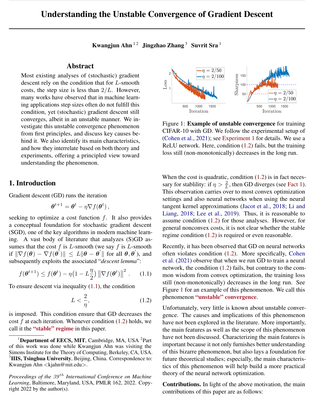
For an $L$ -smooth objective and a stable step size $0<\eta<2/L$ , the descent lemma gives $\mathrm{RP}(\theta)\le -(1-L\eta/2)<0$ whenever $\nabla f(\theta)\ne0$ . In the paper’s CIFAR-10 full-batch GD experiments, step sizes in the unstable regime instead produced relative-progress values oscillating near zero while training loss decreased over the long run, non-monotonically. This is an observed characterization, not a guarantee that every unstable GD trajectory converges; the experiments also show that a sufficiently large step size can still cause divergence.
Knowl 4 — Directional smoothness quantifies oscillation of GD iterates
definition
For a differentiable objective $f$ , parameter $\theta$ , and nonzero update vector $v$ , define directional smoothness by $L(\theta;v)=\langle v,\nabla f(\theta)-\nabla f(\theta-v)\rangle/\|v\|^2$ . For GD, $v=\eta\nabla f(\theta)$ . If the gradient at the updated parameter points in nearly the opposite direction to the gradient at $\theta$ when projected along the update, then $\langle v,\nabla f(\theta-v)\rangle\approx-\langle v,\nabla f(\theta)\rangle$ , and consequently $L(\theta;\eta\nabla f(\theta))\approx2/\eta$ . The paper uses values near $2/\eta$ as a quantitative signature of oscillatory movement, rather than monotone stabilization.
Knowl 5 — Near-zero relative progress implies high curvature along the update segment
theoretical result
Let $f$ be twice differentiable along the GD segment from $\theta^t$ to $\theta^{t+1}=\theta^t-\eta\nabla f(\theta^t)$ , and let $L_t=\sup_{\theta\in[\theta^t,\theta^{t+1}]}\lambda_{\max}(\nabla^2 f(\theta))$ , where $[\theta^t,\theta^{t+1}]$ denotes the line segment. Then $\frac{2}{\eta}(\mathrm{RP}(\theta^t)+1)\le L_t$ . Therefore, when relative progress is near zero, the maximum Hessian eigenvalue somewhere along the update segment must be at least approximately $2/\eta$ . The paper further argues conditionally that if directional smoothness varies little along the segment, the Hessian’s maximum eigenvalue at the current iterate is above this threshold; approximate equality additionally requires the gradient to be approximately aligned with the top Hessian eigenvector.
Knowl 6 — Weight decay can eliminate stationary points in positively homogeneous parameters
theoretical result
Consider a neural-network objective $\ell(\theta)=\frac1n\sum_{i=1}^n f(x_i,\theta)+\gamma\|\theta\|_2^2$ with $\gamma>0$ , and partition parameters as $\theta=[\xi;\zeta]$ . Suppose the data-fit term is invariant to every positive rescaling of the parameter subset $\zeta$ : $f(x_i,[\xi,c\zeta])=f(x_i,[\xi,\zeta])$ for all data points $x_i$ and all $c>0$ . Then $\ell$ has no stationary point with $\zeta\ne0$ . The result supplies one mechanism by which neural-network objectives with weight decay may lack nontrivial stationary points in parameter regions relevant to GD.
Knowl 7 — Flattening can make unstable GD remain in a forward-invariant region
model/method
A mechanism proposed for long-run loss decrease with an unstable step size is the existence of a compact set $S$ satisfying $F(S)\subseteq S$ for the GD map $F(\theta)=\theta-\eta\nabla f(\theta)$ . Flattening the objective away from a minimum can make gradients small enough for such a region to remain invariant, even if a quadratic objective with the same local geometry would diverge. For example, applying $\tanh$ to the quadratic $20\theta_1^2+\theta_2^2$ yields $\tanh(20\theta_1^2+\theta_2^2)$ ; the paper reports non-divergent GD at $\eta=2/39$ , which exceeds the quadratic stability threshold $2/40$ . In a single-neuron fitting example initialized at $(13,0.01)$ with $\eta=2/150$ , the linear network with loss $(\theta_1\theta_2)^2$ diverges, whereas the network with loss $(\theta_1\tanh(\theta_2))^2$ converges to a minimum with sharpness approximately $2/\eta$ . These examples illustrate the proposed role of flattening and activation functions; they do not establish a general convergence theorem.
Knowl 8 — SGD has an expected relative-progress identity
equation
Let $f$ be differentiable, let $g(\theta)$ be a random stochastic gradient satisfying $\mathbb{E}[g(\theta)]=\nabla f(\theta)$ , and let $\eta>0$ with $\nabla f(\theta)\ne0$ . Define expected relative progress as $\mathbb{E}[\mathrm{RP}(\theta)]=[\mathbb{E}f(\theta-\eta g(\theta))-f(\theta)]/[\eta\|\nabla f(\theta)\|^2]$ . With $L(\theta;v)=\langle v,\nabla f(\theta)-\nabla f(\theta-v)\rangle/\|v\|^2$ , the exact relation is $\mathbb{E}[\mathrm{RP}(\theta)]=-1+\frac{\eta}{2}\,2\int_0^1\tau\,\mathbb{E}\!\left[\frac{\|g(\theta)\|^2}{\|\nabla f(\theta)\|^2}L(\theta;\eta\tau g(\theta))\right]d\tau$ . When the directional-smoothness term varies little over $\tau\in[0,1]$ , the paper uses the approximation $\mathbb{E}[\mathrm{RP}(\theta)]\approx-1+\frac{\eta}{2}\mathbb{E}[\frac{\|g(\theta)\|^2}{\|\nabla f(\theta)\|^2}L(\theta;\eta g(\theta))]$ . In CIFAR-10 experiments with ReLU and tanh networks, the measured sides of this approximation were similar. In a ReLU SGD experiment with minibatches of 32 and $\eta=2/100$ , expected relative progress was not consistently below zero even though the loss decreased over the long run.
Knowl 9 — CIFAR-10 experiments support the directional-smoothness approximation across networks
empirical result
In a CIFAR-10 full-batch GD experiment using 5,000 examples, cross-entropy loss, and a fully connected network with two hidden layers of width 200, the paper evaluated $L(\theta^t;\eta\tau\nabla f(\theta^t))$ at $\tau=0.01,0.02,\ldots,1$ every five iterations with $\eta=2/60$ . These measurements varied relatively little across $\tau$ , supporting the approximation $\mathrm{RP}(\theta)\approx-1+\frac{\eta}{2}L(\theta;\eta\nabla f(\theta))$ derived from the exact weighted-integral identity. The paper reports similar behavior for ReLU networks with two or four hidden layers of width 200 and for tanh networks. In a separate comparison under the same 5,000-example, two-hidden-layer setup with $\eta=2/30$ , full-batch GD converged for tanh and ReLU activations but diverged for the network without activations.
Knowl 10 — The characterizations do not cover adaptive optimizers
limitation
The paper’s characterizations concern gradient descent and stochastic gradient descent with constant step size. It does not establish whether the relative-progress, directional-smoothness, or sharpness relationships carry over to adaptive methods such as Adam or RMSProp; their behavior is left as an open direction.

Coverage note — No substantial contributed material is omitted; proof details and background material are excluded, while the central theory, mechanisms, characterizations, and experimental evidence are represented.

References

1.S. Arora, Z. Li, and A. Panigrahi. Understanding gradient descent on edge of stability in deep learning. To appear at International Conference on Machine Learning (ICML) 2022 arXiv:2205.09745, 2022.
2.J. Cohen, S. Kaur, Y. Li, J. Z. Kolter, and A. Talwalkar. Gradient descent on neural networks typically occurs at the edge of stability. In International Conference on Learning Representations, 2021.
3.A. Jacot, F. Gabriel, and C. Hongler. Neural tangent kernel: convergence and generalization in neural networks. In Proceedings of the 32nd Advances in Neural Information Processing Systems, pages 8580–8589, 2018.
4.S. Jastrzkebski, Z. Kenton, D. Arpit, N. Ballas, A. Fischer, Y. Bengio, and A. Storkey. Three factors influencing minima in SGD. arXiv preprint arXiv:1711.04623, 2017.
5.S. Jastrzkebski, Z. Kenton, N. Ballas, A. Fischer, Y. Bengio, and A. Storkey. On the relation between the sharpest directions of dnn loss and the sgd step length. arXiv preprint arXiv:1807.05031, 2018.
6.J. Lee, L. Xiao, S. Schoenholz, Y. Bahri, R. Novak, J. Sohl-Dickstein, and J. Pennington. Wide neural networks of any depth evolve as linear models under gradient descent. Advances in Neural Information Processing Systems, 32: 8572–8583, 2019.
7.J. D. Lee, M. Simchowitz, M. I. Jordan, and B. Recht. Gradient descent only converges to minimizers. In Conference on learning theory, pages 1246–1257. PMLR, 2016.
8.A. Lewkowycz, Y. Bahri, E. Dyer, J. Sohl-Dickstein, and G. Gur-Ari. The large learning rate phase of deep learning: the catapult mechanism. arXiv preprint arXiv:2003.02218, 2020.
9.Y. Li and Y. Liang. Learning overparameterized neural networks via stochastic gradient descent on structured data. In Proceedings of the 32nd International Conference on Neural Information Processing Systems, pages 8168–8177, 2018.
10.C. Ma, D. Kunin, L. Wu, and L. Ying. The multiscale structure of neural network loss functions: The effect on optimization and origin. arXiv preprint arXiv:2204.11326, 2022.
11.I. Panageas and G. Piliouras. Gradient descent only converges to minimizers: Non-isolated critical points and invariant regions. In 8th Innovations in Theoretical Computer Science Conference (ITCS 2017). Schloss Dagstuhl-Leibniz-Zentrum fuer Informatik, 2017.
12.M. Shub. Global stability of dynamical systems. Springer Science & Business Media, 2013.
13.L. Wu, C. Ma, et al. How SGD selects the global minima in over-parameterized learning: A dynamical stability perspective. Advances in Neural Information Processing Systems, 31:8279–8288, 2018.
14.C. Xing, D. Arpit, C. Tsirigotis, and Y. Bengio. A walk with SGD. arXiv preprint arXiv:1802.08770, 2018.

Citation

MLA

Ahn, K., et al. “Understanding the Unstable Convergence of Gradient Descent”. International Conference on Machine Learning, vol. 162, 2022, pp. 247–57, https://proceedings.mlr.press/v162/ahn22a.html.

APA

Ahn, K., Zhang, J., & Sra, S. (2022). Understanding the unstable convergence of gradient descent. International Conference on Machine Learning, 162, 247–257. https://proceedings.mlr.press/v162/ahn22a.html

Chicago

Ahn, K., J. Zhang, and S. Sra. 2022. “Understanding the Unstable Convergence of Gradient Descent”. International Conference on Machine Learning 162: 247–57. https://proceedings.mlr.press/v162/ahn22a.html.

Harvard

Ahn, K., Zhang, J. and Sra, S. (2022) “Understanding the unstable convergence of gradient descent”, International Conference on Machine Learning. PMLR, pp. 247–257. Available at: https://proceedings.mlr.press/v162/ahn22a.html.

Vancouver

1. Ahn K, Zhang J, Sra S (2022) Understanding the unstable convergence of gradient descent. In: International Conference on Machine Learning. PMLR, pp 247–257

BibTeX

@InProceedings{pmlr-v162-ahn22a,
  title = 	 {Understanding the unstable convergence of gradient descent},
  author =       {Ahn, Kwangjun and Zhang, Jingzhao and Sra, Suvrit},
  booktitle = 	 {Proceedings of the 39th International Conference on Machine Learning},
  pages = 	 {247--257},
  year = 	 {2022},
  editor = 	 {Chaudhuri, Kamalika and Jegelka, Stefanie and Song, Le and Szepesvari, Csaba and Niu, Gang and Sabato, Sivan},
  volume = 	 {162},
  series = 	 {Proceedings of Machine Learning Research},
  month = 	 {17--23 Jul},
  publisher =    {PMLR},
  pdf = 	 {https://proceedings.mlr.press/v162/ahn22a/ahn22a.pdf},
  url = 	 {https://proceedings.mlr.press/v162/ahn22a.html},
  abstract = 	 {Most existing analyses of (stochastic) gradient descent rely on the condition that for $L$-smooth costs, the step size is less than $2/L$. However, many works have observed that in machine learning applications step sizes often do not fulfill this condition, yet (stochastic) gradient descent still converges, albeit in an unstable manner. We investigate this unstable convergence phenomenon from first principles, and discuss key causes behind it. We also identify its main characteristics, and how they interrelate based on both theory and experiments, offering a principled view toward understanding the phenomenon.}
}

Metadata:DOI registry

Access the Paper

This paper is available from its original source. Click below to access the PDF.

Open PDF

License: https://creativecommons.org/licenses/by/4.0/

Understanding the unstable convergence of gradient descent

Abstract

Keywords

Table of Contents

Knowls

Knowl 1 — Almost all GD initializations avoid unstable stationary points

Knowl 2 — Relative progress is exactly linked to directional smoothness

Knowl 3 — Relative progress distinguishes stable from unstable GD behavior

Knowl 4 — Directional smoothness quantifies oscillation of GD iterates

Knowl 5 — Near-zero relative progress implies high curvature along the update segment

Knowl 6 — Weight decay can eliminate stationary points in positively homogeneous parameters

Knowl 7 — Flattening can make unstable GD remain in a forward-invariant region

Knowl 8 — SGD has an expected relative-progress identity

Knowl 9 — CIFAR-10 experiments support the directional-smoothness approximation across networks

Knowl 10 — The characterizations do not cover adaptive optimizers

References

Citation

BibTeX

Access the Paper