A Differential Equation for Modeling Nesterov's Accelerated Gradient Method: Theory and Insights cover

📄 Executive Summary

Modern data analysis and machine learning rely heavily on convex optimization to train large-scale computational models. While Nesterov's accelerated gradient method has served as an industry standard for decades due to its optimal convergence rate, its exact mathematical mechanics have remained difficult to analyze, interpret, and adapt. The algorithm exhibits non-monotonic behaviors, such as persistent oscillations and overshoots around the target solution, which complicate performance guarantees in practical settings.

The article establishes a continuous-time ordinary differential equation that acts as the exact physical limit of Nesterov's scheme as step sizes become infinitesimal. By transforming discrete algorithmic steps into a continuous dynamical system, the article evaluates the underlying mechanics of acceleration and provides analytical tools to explain, improve, and generalize accelerated first-order optimization algorithms.

To conduct this evaluation, the authors performed rigorous mathematical analysis using energy functionals, physical damping models, and Bessel function solutions. They validated these analytical findings across diverse numerical simulations, including synthetic Lasso problems, nonnegative least squares, matrix completion, and regularized logistic regression under both standard and high-dimensional sparse conditions.

The analysis yields four critical findings. First, Nesterov's discrete algorithm converges precisely to a second-order differential equation exhibiting a time-dependent friction term. Second, the algorithm behaves as an overdamped system early on and transitions into an underdamped system over time, which mathematically explains why iterates oscillate and overshoot the minimizer at later stages. Third, the parameter defining the friction exhibits a strict threshold: setting this friction parameter to at least three guarantees the optimal inverse quadratic convergence rate, whereas lower values fail to achieve acceleration. Fourth, the article introduces a speed-based restarting scheme that resets momentum whenever iterate velocity decreases, provably attaining a linear convergence rate on strongly convex functions without requiring prior knowledge of problem conditioning.

These findings provide immediate practical implications for engineering and machine learning pipelines. By framing optimization algorithms as physical damping systems, developers gain intuitive design principles to eliminate performance-degrading trajectory oscillations. The proposed speed restarting scheme substantially reduces computational runtimes and resource consumption while achieving robust, stable convergence across smooth, composite, and non-smooth optimization tasks.

Organizations implementing accelerated first-order methods should incorporate speed-based restarting into their numerical solvers to accelerate convergence and eliminate costly overshoot cycles. Practitioners tuning generalized acceleration schemes should ensure their damping parameter remains at or above the critical value of three. Future work should focus on extending continuous-time mapping frameworks to systematically translate ordinary differential equation properties back into discrete algorithms, as well as establishing theoretical convergence rates for alternative heuristic restart mechanisms.

Confidence in these theoretical results is high, supported by complete mathematical proofs and robust empirical benchmarks across varied problem classes. Readers should note that while the theoretical linear convergence rate for the speed restarting scheme is rigorously proven for strongly convex functions, empirical tests also demonstrate strong performance on non-strongly convex and non-smooth functions where theoretical guarantees remain an active area of investigation.

📚 What to read before this

On the importance of initialization and momentum in deep learning, Ilya Sutskever et al. (2013). This work demonstrates the practical importance of momentum schedules and Nesterov acceleration in deep learning, providing empirical motivation for modeling Nesterov's scheme through continuous dynamical systems.
Stochastic First- and Zeroth-Order Methods for Nonconvex Stochastic Programming, Saeed Ghadimi et al. (2013). This paper establishes foundational complexity and convergence analysis for first-order stochastic optimization methods that underpin accelerated gradient techniques.
The Tradeoffs of Large Scale Learning, Léon Bottou et al. (2007). It lays out the foundational computational trade-offs between asymptotic convergence rates and large-scale learning bottlenecks that motivate optimal accelerated first-order algorithms.

📚 What to read after this

Improved Gradient Descent Lower Bounds Beyond Nesterov, Yuhan Ye et al. (2026). This work directly explores theoretical limits and lower bounds on gradient descent schedules relative to Nesterov's optimal acceleration rate.
SGDR: Stochastic Gradient Descent with Warm Restarts, Ilya Loshchilov et al. (2016). It extends the concept of dynamic restart mechanisms in first-order optimization by developing periodic warm restarts with cosine learning rate schedules.
An overview of gradient descent optimization algorithms, Sebastian Ruder (2016). It provides a comprehensive survey connecting momentum and Nesterov accelerated gradient methods to subsequent adaptive first-order optimization algorithms.
Optimization Methods for Large-Scale Machine Learning, Léon Bottou et al. (2016). It synthesizes modern first-order, momentum, and stochastic optimization techniques across large-scale machine learning applications.

A Differential Equation for Modeling Nesterov’s Accelerated Gradient Method: Theory and Insights

Weijie Su
Department of Statistics
Stanford University
Stanford, CA 94305, USA

Stephen Boyd
Department of Electrical Engineering
Stanford University
Stanford, CA 94305, USA

Emmanuel J. Candès
Departments of Statistics and Mathematics
Stanford University
Stanford, CA 94305, USA

Abstract

We derive a second-order ordinary differential equation (ODE) which is the limit of Nesterov’s accelerated gradient method. This ODE exhibits approximate equivalence to Nesterov’s scheme and thus can serve as a tool for analysis. We show that the continuous time ODE allows for a better understanding of Nesterov’s scheme. As a byproduct, we obtain a family of schemes with similar convergence rates. The ODE interpretation also suggests restarting Nesterov’s scheme leading to an algorithm, which can be rigorously proven to converge at a linear rate whenever the objective is strongly convex.

Executive Summary: Modern data analysis and machine learning rely heavily on convex optimization to train large-scale computational models. While Nesterov's accelerated gradient method has served as an industry standard for decades due to its optimal convergence rate, its exact mathematical mechanics have remained difficult to analyze, interpret, and adapt. The algorithm exhibits non-monotonic behaviors, such as persistent oscillations and overshoots around the target solution, which complicate performance guarantees in practical settings.

The article establishes a continuous-time ordinary differential equation that acts as the exact physical limit of Nesterov's scheme as step sizes become infinitesimal. By transforming discrete algorithmic steps into a continuous dynamical system, the article evaluates the underlying mechanics of acceleration and provides analytical tools to explain, improve, and generalize accelerated first-order optimization algorithms.

To conduct this evaluation, the authors performed rigorous mathematical analysis using energy functionals, physical damping models, and Bessel function solutions. They validated these analytical findings across diverse numerical simulations, including synthetic Lasso problems, nonnegative least squares, matrix completion, and regularized logistic regression under both standard and high-dimensional sparse conditions.

The analysis yields four critical findings. First, Nesterov's discrete algorithm converges precisely to a second-order differential equation exhibiting a time-dependent friction term. Second, the algorithm behaves as an overdamped system early on and transitions into an underdamped system over time, which mathematically explains why iterates oscillate and overshoot the minimizer at later stages. Third, the parameter defining the friction exhibits a strict threshold: setting this friction parameter to at least three guarantees the optimal inverse quadratic convergence rate, whereas lower values fail to achieve acceleration. Fourth, the article introduces a speed-based restarting scheme that resets momentum whenever iterate velocity decreases, provably attaining a linear convergence rate on strongly convex functions without requiring prior knowledge of problem conditioning.

These findings provide immediate practical implications for engineering and machine learning pipelines. By framing optimization algorithms as physical damping systems, developers gain intuitive design principles to eliminate performance-degrading trajectory oscillations. The proposed speed restarting scheme substantially reduces computational runtimes and resource consumption while achieving robust, stable convergence across smooth, composite, and non-smooth optimization tasks.

Organizations implementing accelerated first-order methods should incorporate speed-based restarting into their numerical solvers to accelerate convergence and eliminate costly overshoot cycles. Practitioners tuning generalized acceleration schemes should ensure their damping parameter remains at or above the critical value of three. Future work should focus on extending continuous-time mapping frameworks to systematically translate ordinary differential equation properties back into discrete algorithms, as well as establishing theoretical convergence rates for alternative heuristic restart mechanisms.

Confidence in these theoretical results is high, supported by complete mathematical proofs and robust empirical benchmarks across varied problem classes. Readers should note that while the theoretical linear convergence rate for the speed restarting scheme is rigorously proven for strongly convex functions, empirical tests also demonstrate strong performance on non-strongly convex and non-smooth functions where theoretical guarantees remain an active area of investigation.

1. Introduction

Section Summary: This introduction discusses how minimizing convex functions lies at the heart of many machine learning tasks and reviews classical algorithms, with special focus on Nesterov’s accelerated gradient method that improves convergence speed through a carefully chosen momentum term. The authors show that, in the limit of small step sizes, Nesterov’s discrete iteration converges to a simple second-order differential equation whose solutions exhibit the same optimal convergence rate. They argue that this continuous view offers an intuitive framework for understanding observed oscillations in the iterates and for analyzing or extending the original scheme.

In many fields of machine learning, minimizing a convex function is at the core of efficient model estimation. In the simplest and most standard form, we are interested in solving

$ \text{minimize}\quad f(x), $

where $f$ is a convex function, smooth or non-smooth, and $x \in \mathbb{R}^n$ is the variable. Since Newton, numerous algorithms and methods have been proposed to solve the minimization problem, notably gradient and subgradient descent, Newton's methods, trust region methods, conjugate gradient methods, and interior point methods (see e.g. [1, 2, 3, 4, 5, 6, 7] for expositions).

First-order methods have regained popularity as data sets and problems are ever increasing in size and, consequently, there has been much research on the theory and practice of accelerated first-order schemes. Perhaps the earliest first-order method for minimizing a convex function $f$ is the gradient method, which dates back to Euler and Lagrange. Thirty years ago, however, in a seminal paper Nesterov proposed an accelerated gradient method ([8]), which may take the following form: starting with $x_0$ and $y_0 = x_0$, inductively define

$ \begin{aligned} & x_k = y_{k-1} - s\nabla f(y_{k-1})\ & y_k = x_k + \frac{k-1}{k+2} (x_k - x_{k-1}). \end{aligned} $

For any fixed step size $s \le 1/L$, where $L$ is the Lipschitz constant of $\nabla f$, this scheme exhibits the convergence rate

$ f(x_k) - f^\star \le O \left(\frac{|x_0 - x^\star|^2}{sk^2} \right). $

Above, $x^\star$ is any minimizer of $f$ and $f^\star = f(x^\star)$. It is well-known that this rate is optimal among all methods having only information about the gradient of $f$ at consecutive iterates ([9]). This is in contrast to vanilla gradient descent methods, which have the same computational complexity but can only achieve a rate of $O(1/k)$. This improvement relies on the introduction of the momentum term $x_k-x_{k-1}$ as well as the particularly tuned coefficient $(k-1)/(k+2)\approx 1 - 3/k$. Since the introduction of Nesterov's scheme, there has been much work on the development of first-order accelerated methods, see [9, 10, 11] for theoretical developments, and [12] for a unified analysis of these ideas. Notable applications can be found in sparse linear regression ([13, 14]), compressed sensing ([15]) and, deep and recurrent neural networks ([16]).

In a different direction, there is a long history relating ordinary differential equation (ODEs) to optimization, see [17], [18], and [19] for example. The connection between ODEs and numerical optimization is often established via taking step sizes to be very small so that the trajectory or solution path converges to a curve modeled by an ODE. The conciseness and well-established theory of ODEs provide deeper insights into optimization, which has led to many interesting findings. Notable examples include linear regression via solving differential equations induced by linearized Bregman iteration algorithm ([20]), a continuous-time Nesterov-like algorithm in the context of control design ([21, 22]), and modeling design iterative optimization algorithms as nonlinear dynamical systems ([23]).

In this work, we derive a second-order ODE which is the exact limit of Nesterov's scheme by taking small step sizes in Equation 1; to the best of our knowledge, this work is the first to use ODEs to model Nesterov's scheme or its variants in this limit. One surprising fact in connection with this subject is that a first-order scheme is modeled by a second-order ODE. This ODE takes the following form:

$ \ddot{X} + \frac{3}{t}\dot{X} + \nabla f(X) = 0 $

for $t > 0$, with initial conditions $X(0) = x_0, \dot{X}(0) = 0$; here, $x_0$ is the starting point in Nesterov's scheme, $\dot{X} \equiv {\mathrm{d}} X/{\mathrm{d}} t$ denotes the time derivative or velocity and similarly $\ddot{X} \equiv {\mathrm{d}}^2 X/{\mathrm{d}} t^2$ denotes the acceleration. The time parameter in this ODE is related to the step size in Equation 1 via $t \approx k\sqrt{s}$. Expectedly, it also enjoys inverse quadratic convergence rate as its discrete analog,

$ f(X(t)) - f^\star \le O\left( \frac{|x_0 - x^\star|^2}{t^2}\right). $

Approximate equivalence between Nesterov's scheme and the ODE is established later in various perspectives, rigorous and intuitive. In the main body of this paper, examples and case studies are provided to demonstrate that the homogeneous and conceptually simpler ODE can serve as a tool for understanding, analyzing and generalizing Nesterov's scheme.

In the following, two insights of Nesterov's scheme are highlighted, the first one on oscillations in the trajectories of this scheme, and the second on the peculiar constant 3 appearing in the ODE.

1.1 From Overdamping to Underdamping

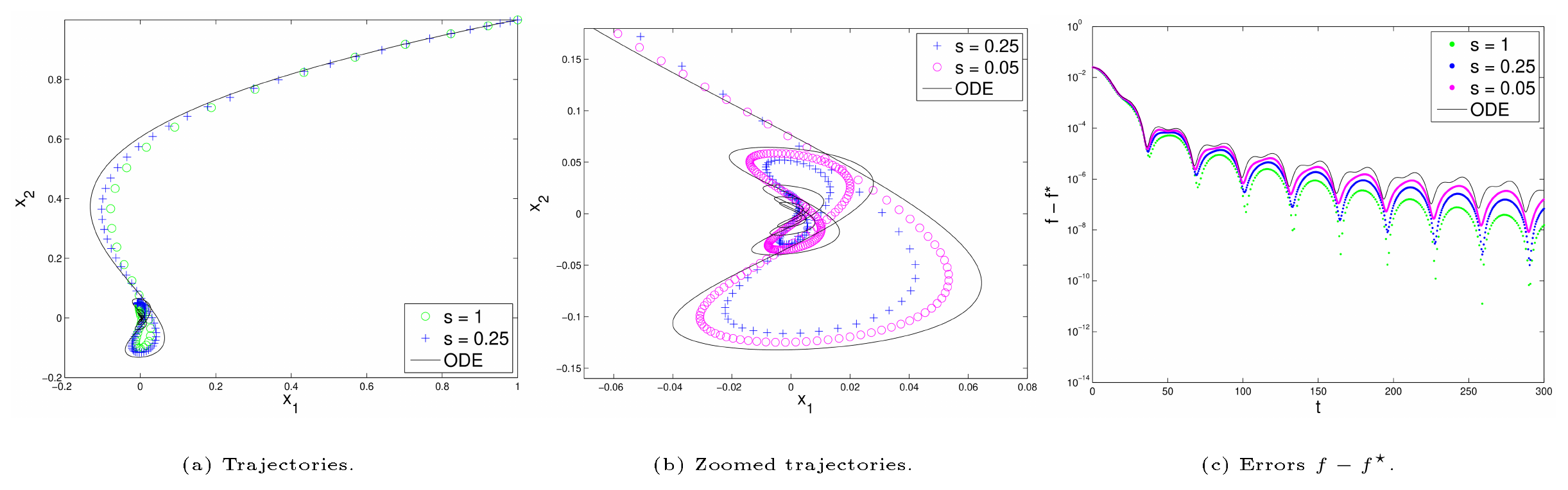
In general, Nesterov's scheme is not monotone in the objective function value due to the introduction of the momentum term. Oscillations or overshoots along the trajectory of iterates approaching the minimizer are often observed when running Nesterov's scheme. Figure 1 presents typical phenomena of this kind, where a two-dimensional convex function is minimized by Nesterov's scheme. Viewing the ODE as a damping system, we obtain interpretations as follows.

Small $t$. In the beginning, the damping ratio $3/t$ is large. This leads the ODE to be an overdamped system, returning to the equilibrium without oscillating;

Large $t$. As $t$ increases, the ODE with a small $3/t$ behaves like an underdamped system, oscillating with the amplitude gradually decreasing to zero.

As depicted in Figure 1a, in the beginning the ODE curve moves smoothly towards the origin, the minimizer $x^\star$. The second interpretation ``Large $t

#39;' provides partial explanation for the oscillations observed in Nesterov's scheme at later stage. Although our analysis extends farther, it is similar in spirit to that carried in [24]. In particular, the zoomed Figure 1b presents some butterfly-like oscillations for both the scheme and ODE. There, we see that the trajectory constantly moves away from the origin and returns back later. Each overshoot in Figure 1b causes a bump in the function values, as shown in Figure 1c. We observe also from Figure 1c that the periodicity captured by the bumps are very close to that of the ODE solution. In passing, it is worth mentioning that the solution to the ODE in this case can be expressed via Bessel functions, hence enabling quantitative characterizations of these overshoots and bumps, which are given in full detail in Section 3.

$**Figure 1:** Minimizing $f = 2\times 10^{-2} x_1^2 + 5\times 10^{-3} x_2^2$, starting from $x_0 = (1, ~ 1)$. The black and solid curves correspond to the solution to the ODE. In (c), for the x-axis we use the identification between time and iterations, $t = k\sqrt{s}$.$

1.2 A Phase Transition

The constant 3, derived from $(k+2) - (k-1)$ in Equation 3, is not haphazard. In fact, it is the smallest constant that guarantees $O(1/t^2)$ convergence rate. Specifically, parameterized by a constant $r$, the generalized ODE

$ \ddot{X} + \frac{r}{t}\dot{X} + \nabla f(X) = 0 $

can be translated into a generalized Nesterov's scheme that is the same as the original Equation 1 except for $(k-1)/(k+2)$ being replaced by $(k-1)/(k+r-1)$. Surprisingly, for both generalized ODEs and schemes, the inverse quadratic convergence is guaranteed if and only if $r \ge 3$. This phase transition suggests there might be deep causes for acceleration among first-order methods. In particular, for $r \ge 3$, the worst case constant in this inverse quadratic convergence rate is minimized at $r = 3$.

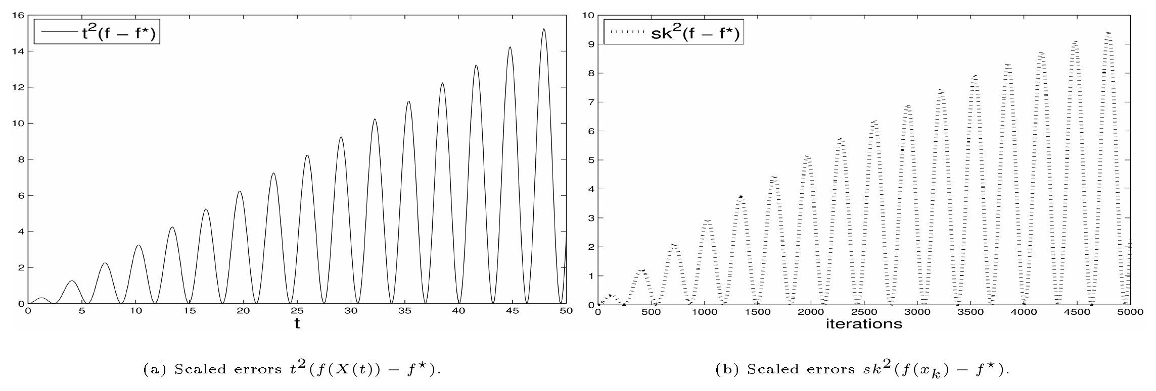
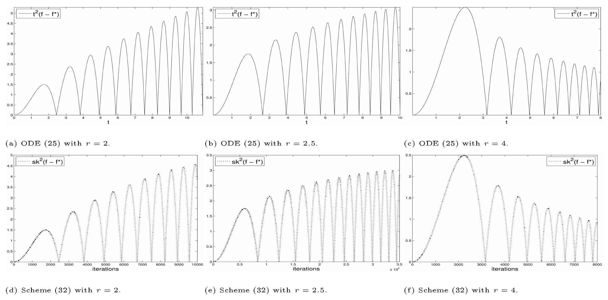
Figure 2 illustrates the growth of $t^2(f(X(t)) - f^\star)$ and $sk^2(f(x_k) - f^\star)$, respectively, for the generalized ODE and scheme with $r = 1$, where the objective function is simply $f(x) = \frac12 x^2$. Inverse quadratic convergence fails to be observed in both Figure 2a and Figure 2b, where the scaled errors grow with $t$ or iterations, for both the generalized ODE and scheme.

$**Figure 2:** Minimizing $f = \frac12 x^2$ by the generalized ODE and scheme with $r = 1$, starting from $x_0 = 1$. In (b), the step size $s = 10^{-4}$.$

1.3 Outline and Notation

The rest of the paper is organized as follows. In Section 2, the ODE is rigorously derived from Nesterov's scheme, and a generalization to composite optimization, where $f$ may be non-smooth, is also obtained. Connections between the ODE and the scheme, in terms of trajectory behaviors and convergence rates, are summarized in Section 3. In Section 4, we discuss the effect of replacing the constant $3$ in Equation 3 by an arbitrary constant on the convergence rate. A new restarting scheme is suggested in Section 5, with linear convergence rate established and empirically observed.

Some standard notations used throughout the paper are collected here. We denote by $\mathcal{F}_L$ the class of convex functions $f$ with $L$–Lipschitz continuous gradients defined on $\mathbb{R}^n$, i.e., $f$ is convex, continuously differentiable, and satisfies

$ |\nabla f(x) - \nabla f(y)| \le L|x - y| $

for any $x, y\in \mathbb{R}^n$, where $|\cdot|$ is the standard Euclidean norm and $L > 0$ is the Lipschitz constant. Next, $\mathcal{S}{\mu}$ denotes the class of $\mu$–strongly convex functions $f$ on $\mathbb{R}^n$ with continuous gradients, i.e., $f$ is continuously differentiable and $f(x) - \mu|x|^2/2$ is convex. We set $\mathcal{S}{\mu,L} = \mathcal{F}{L}\cap \mathcal{S}{\mu}$.

2. Derivation

Section Summary: The section derives a second-order ODE that approximates Nesterov's accelerated gradient method in the continuous-time limit of vanishing step size. Starting from the discrete recurrence, the authors posit that the iterates track a smooth trajectory X(t), substitute a Taylor expansion in the step size, and match leading-order terms to obtain the differential equation (\ddot{X} + (3/t)\dot{X} + \nabla f(X) = 0) together with the initial conditions X(0) = x_0 and (\dot{X}(0) = 0). They then establish existence and uniqueness of a global solution, prove that the discrete sequence converges uniformly to this trajectory on finite time intervals, and note several invariance properties and the short-time asymptotic X(t) ≈ x_0 − (t²/8)∇f(x_0).

First, we sketch an informal derivation of the ODE Equation 3. Assume $f\in \mathcal{F}_L$ for $L > 0$. Combining the two equations of Equation 1 and applying a rescaling gives

$ \frac{x_{k+1} -x_k}{\sqrt{s}} = \frac{k-1}{k+2}\frac{x_k -x_{k-1}}{\sqrt{s}} - \sqrt{s}\nabla f(y_k). $

Introduce the Ansatz $x_k \approx X(k\sqrt{s})$ for some smooth curve $X(t)$ defined for $t \ge 0$. Put $k = t/\sqrt{s}$. Then as the step size $s$ goes to zero, $X(t) \approx x_{t/\sqrt{s}} = x_k$ and $X(t+\sqrt{s} ) \approx x_{(t+\sqrt{s})/\sqrt{s}} = x_{k+1}$, and Taylor expansion gives

$ (x_{k+1} -x_k)/ \sqrt{s} = \dot{X}(t) + \frac{1}{2}\ddot{X}(t)\sqrt{s} + o(\sqrt{s}), \quad (x_{k} -x_{k-1})/ \sqrt{s} = \dot{X}(t) - \frac{1}{2}\ddot{X}(t)\sqrt{s} + o(\sqrt{s}) $

and $\sqrt{s}\nabla f(y_k) = \sqrt{s}\nabla f(X(t)) + o(\sqrt{s})$. Thus Equation 4 can be written as

$ \begin{split} \dot{X}(t) + \frac{1}{2}\ddot{X}(t)\sqrt{s} + o(\sqrt{s})\ = \Big(1 - \frac{3\sqrt{s}}{t} \Big) \Big(\dot{X}(t) - \frac{1}{2}\ddot{X}(t)\sqrt{s} + o(\sqrt{s}) \Big) - \sqrt{s}\nabla f(X(t)) + o(\sqrt{s}). \end{split} $

By comparing the coefficients of $\sqrt{s}$ in Equation 5, we obtain

$ \nonumber \ddot{X} + \frac{3}{t}\dot{X} + \nabla f(X) = 0. $

The first initial condition is $X(0) = x_0$. Taking $k=1$ in Equation 4 yields

$ (x_2-x_1)/\sqrt{s} = -\sqrt{s}\nabla f(y_1) = o(1). $

Hence, the second initial condition is simply $\dot{X}(0) = 0$ (vanishing initial velocity).

One popular alternative momentum coefficient is $\theta_k(\theta_{k-1}^{-1} - 1)$, where $\theta_k$ are iteratively defined as $\theta_{k+1} = \left(\sqrt{\theta_k^4 + 4\theta_k^2} - \theta_k^2 \right)/2$, starting from $\theta_0 = 1$ ([8, 13]). Simple analysis reveals that $\theta_k(\theta_{k-1}^{-1} - 1)$ asymptotically equals $1 - 3/k + O(1/k^2)$, thus leading to the same ODE as Equation 1.

Classical results in ODE theory do not directly imply the existence or uniqueness of the solution to this ODE because the coefficient $3/t$ is singular at $t=0$. In addition, $\nabla f$ is typically not analytic at $x_0$, which leads to the inapplicability of the power series method for studying singular ODEs. Nevertheless, the ODE is well posed: the strategy we employ for showing this constructs a series of ODEs approximating Equation 3, and then chooses a convergent subsequence by some compactness arguments such as the Arzelá-Ascoli theorem. Below, $C^{2}((0,\infty); \mathbb{R}^n)$ denotes the class of twice continuously differentiable maps from $(0, \infty)$ to $\mathbb{R}^n$; similarly, $C^{1}([0,\infty); \mathbb{R}^n)$ denotes the class of continuously differentiable maps from $[0, \infty)$ to $\mathbb{R}^n$.

########## {caption="Theorem 1"}

For any $f\in\mathcal{F}{\infty} := \cup{L > 0}\mathcal{F}_L$ and any $x_0\in \mathbb{R}^n$, the ODE Equation 3 with initial conditions $X(0) = x_0, \dot{X}(0) = 0$ has a unique global solution $X\in C^{2}((0,\infty); \mathbb{R}^n)\cap C^{1}([0,\infty); \mathbb{R}^n)$.

The next theorem, in a rigorous way, guarantees the validity of the derivation of this ODE. The proofs of both theorems are deferred to the appendices.

########## {caption="Theorem 2"}

For any $f \in \mathcal{F}_{\infty}$, as the step size $s \rightarrow 0$, Nesterov's scheme Equation 1 converges to the ODE Equation 3 in the sense that for all fixed $T > 0$,

$ \lim_{s \rightarrow 0}\max_{0 \le k \le \frac{T}{\sqrt{s}}}\left| x_k - X\left( k\sqrt{s} \right) \right| = 0. $

2.1 Simple Properties

We collect some elementary properties that are helpful in understanding the ODE.

Time Invariance. If we adopt a linear time transformation, $\tilde{t} = ct$ for some $c > 0$, by the chain rule it follows that

$ \frac{{\mathrm{d}} X}{{\mathrm{d}} \tilde{t}} = \frac{1}{c}\frac{{\mathrm{d}} X}{{\mathrm{d}} t}, ~ \frac{{\mathrm{d}}^2 X}{{\mathrm{d}} \tilde{t}^2} = \frac{1}{c^2}\frac{{\mathrm{d}}^2 X}{{\mathrm{d}} t^2}. $

This yields the ODE parameterized by $\tilde{t}$,

$ \nonumber \frac{{\mathrm{d}}^2 X}{{\mathrm{d}} \tilde{t}^2} + \frac{3}{\tilde{t}}\frac{{\mathrm{d}} X}{{\mathrm{d}} \tilde{t}} + \nabla f(X)/c^2 = 0. $

Also note that minimizing $f/c^2$ is equivalent to minimizing $f$. Hence, the ODE is invariant under the time change. In fact, it is easy to see that time invariance holds if and only if the coefficient of $\dot{X}$ has the form $C/t$ for some constant $C$.

Rotational Invariance. Nesterov's scheme and other gradient-based schemes are invariant under rotations. As expected, the ODE is also invariant under orthogonal transformation. To see this, let $Y = QX$ for some orthogonal matrix $Q$. This leads to $\dot{Y} = Q\dot{X}, \ddot{Y} = Q\ddot{X}$ and $\nabla_Y f = Q\nabla_X f$. Hence, denoting by $Q^T$ the transpose of $Q$, the ODE in the new coordinate system reads $Q^T\ddot{Y} + \frac{3}{t}Q^T\dot{Y} + Q^T\nabla_Yf = 0$, which is of the same form as Equation 3 once multiplying $Q$ on both sides.

Initial Asymptotic. Assume sufficient smoothness of $X$ such that $\lim_{t \rightarrow 0} \ddot{X}(t)$ exists. The mean value theorem guarantees the existence of some $\xi\in(0, t)$ that satisfies $\dot{X}(t)/t = (\dot{X}(t) - \dot{X}(0))/t = \ddot{X}(\xi)$. Hence, from the ODE we deduce $\ddot{X}(t) + 3\ddot{X}(\xi) + \nabla f(X(t)) = 0$. Taking the limit $t \rightarrow 0$ gives $\ddot{X}(0) = -\nabla f(x_0)/4$. Hence, for small $t$ we have the asymptotic form:

$ \nonumber X(t) = - \frac{\nabla f(x_0)t^2}{8} + x_0 + o(t^2). $

This asymptotic expansion is consistent with the empirical observation that Nesterov's scheme moves slowly in the beginning.

2.2 ODE for Composite Optimization

It is interesting and important to generalize the ODE to minimizing $f$ in the composite form $f(x) = g(x) + h(x)$, where the smooth part $g\in \mathcal{F}_{L}$ and the non-smooth part $h: \mathbb{R}^n \rightarrow(-\infty,\infty]$ is a structured general convex function. Both [11] and [13] obtain $O(1/k^2)$ convergence rate by employing the proximal structure of $h$. In analogy to the smooth case, an ODE for composite $f$ is derived in the appendix.

3. Connections and Interpretations

Section Summary: This section shows that a certain ODE closely mirrors Nesterov's accelerated optimization method, both in how quickly they approach a minimum and in how they behave over time. It proves that solutions to the ODE reach the optimum at an inverse-quadratic rate by tracking a simple energy-like quantity that steadily decreases, and it demonstrates that the constant factor in this rate cannot be improved. The authors further use exact solutions for quadratic problems, expressed with Bessel functions, to explain oscillatory behavior and to contrast the method numerically with ordinary gradient descent.

In this section, we explore the approximate equivalence between the ODE and Nesterov's scheme, and provide evidence that the ODE can serve as an amenable tool for interpreting and analyzing Nesterov's scheme. The first subsection exhibits inverse quadratic convergence rate for the ODE solution, the next two address the oscillation phenomenon discussed in Section 1.1, and the last subsection is devoted to comparing Nesterov's scheme with gradient descent from a numerical perspective.

3.1 Analogous Convergence Rate

The original result from [8] states that, for any $f\in\mathcal{F}_L$, the sequence ${x_k}$ given by Equation 1 with step size $s \le 1/L$ satisfies

$ f(x_k) - f^\star \le \frac{2|x_0 - x^\star|^2}{s(k+1)^2}. $

Our next result indicates that the trajectory of Equation 3 closely resembles the sequence ${x_k}$ in terms of the convergence rate to a minimizer $x^\star$. Compared with the discrete case, this proof is shorter and simpler.

########## {caption="Theorem 3"}

For any $f\in\mathcal{F}_{\infty}$, let $X(t)$ be the unique global solution to 3 with initial conditions $X(0) = x_0, \dot{X}(0) = 0$. Then, for any $t > 0$,

$ f(X(t)) - f^\star \le \frac{2|x_0-x^\star|^2}{t^2}. $

Proof: Consider the energy functional[^1] defined as $\mathcal{E}(t) = t^2(f(X(t)) - f^\star) + 2|X + t\dot{X}/2 - x^\star |^2$, whose time derivative is

$ \dot{\mathcal{E}} = 2t(f(X) - f^\star) + t^2\langle \nabla f, \dot{X} \rangle + 4\left\langle X + \frac{t}{2}\dot{X} - x^\star, \frac{3}{2}\dot{X} + \frac{t}{2}\ddot{X} \right\rangle. $

[^1]: We may also view this functional as the negative entropy. Similarly, for the gradient flow $\dot{X} + \nabla f(X) = 0$, an energy function of form $\mathcal{E}_{\mathrm{gradient}}(t) = t(f(X(t))-f^\star) + |X(t) - x^\star|^2/2$ can be used to derive the bound $f(X(t)) - f^\star \le \frac{|x_0-x^\star|^2}{2t}$.

Substituting $3\dot{X}/2 + t\ddot{X}/2$ with $-t\nabla f(X)/2$, the above equation gives

$ \dot{\mathcal{E}} = 2t(f(X) - f^\star) + 4\langle X - x^\star, - t\nabla f(X)/2 \rangle = 2t(f(X) - f^\star) -2t\langle X - x^\star, \nabla f(X) \rangle \le 0, $

where the inequality follows from the convexity of $f$. Hence by monotonicity of $\mathcal{E}$ and non-negativity of $2|X + t\dot{X}/2 - x^\star|^2$, the gap satisfies

$ f(X(t)) - f^\star \le \frac{\mathcal{E}(t)}{t^2} \le \frac{\mathcal{E}(0)}{t^2} = \frac{2|x_0 - x^\star|^2}{t^2}. $

Making use of the approximation $t \approx k\sqrt{s}$, we observe that the convergence rate in Equation 9 is essentially a discrete version of that in Equation 10, providing yet another piece of evidence for the approximate equivalence between the ODE and the scheme.

We finish this subsection by showing that the number 2 appearing in the numerator of the error bound in Equation 10 is optimal. Consider an arbitrary $f \in \mathcal{F}_{\infty}(\mathbb{R})$ such that $f(x) = x$ for $x \ge 0$. Starting from some $x_0 > 0$, the solution to 3 is $X(t) = x_0 - t^2/8$ before hitting the origin. Hence, $t^2(f(X(t)) - f^\star) = t^2(x_0 - t^2/8)$ has a maximum $2x_0^2 = 2|x_0 - 0|^2$ achieved at $t = 2\sqrt{x_0}$. Therefore, we cannot replace 2 by any smaller number, and we can expect that this tightness also applies to the discrete analog Equation 9.

3.2 Quadratic $f$ and Bessel Functions

For quadratic $f$, the ODE Equation 3 admits a solution in closed form. This closed form solution turns out to be very useful in understanding the issues raised in the introduction.

Let $f(x) = \frac12\langle x, Ax \rangle + \langle b, x \rangle$, where $A \in \mathbb{R}^{n \times n}$ is a positive semidefinite matrix and $b$ is in the column space of $A$ because otherwise this function can attain $-\infty$. Then a simple translation in $x$ can absorb the linear term $\langle b, x\rangle$ into the quadratic term. Since both the ODE and the scheme move within the affine space perpendicular to the kernel of $A$, without loss of generality, we assume that $A$ is positive definite, admitting a spectral decomposition $A = Q^T\Lambda Q$, where $\Lambda$ is a diagonal matrix formed by the eigenvalues. Replacing $x$ with $Qx$, we assume $f = \frac12 \langle x, \Lambda x \rangle$ from now on. Now, the ODE for this function admits a simple decomposition of form

$ \nonumber \ddot{X}_i + \frac{3}{t}\dot{X}_i + \lambda_i X_i = 0, \quad i=1,\ldots, n $

with $X_i(0) = x_{0,i}, \dot{X}_i(0) = 0$. Introduce $Y_i(u) = uX_i(u/\sqrt{\lambda_i})$, which satisfies

$ \nonumber u^2\ddot{Y_i} + u\dot{Y_i} + (u^2 - 1)Y_i=0. $

This is Bessel's differential equation of order one. Since $Y_i$ vanishes at $u=0$, we see that $Y_i$ is a constant multiple of $J_1$, the Bessel function of the first kind of order one.[^2] It has an analytic expansion:

$ J_1(u) =\sum_{m=0}^{\infty} \frac{(-1)^m}{(2m)!!(2m+2)!!}u^{2m+1}, $

which gives the asymptotic expansion

$ J_1(u) = (1 + o(1))\frac{u}2 $

when $u \rightarrow 0$. Requiring $X_i(0) = x_{0,i}$, hence, we obtain

[^2]: Up to a constant multiplier, $J_1$ is the unique solution to the Bessel's differential equation $u^2 \ddot{J}_1 + u\dot{J}_1 + (u^2-1)J_1 = 0$ that is finite at the origin. In the analytic expansion of $J_1$, $m !!$ denotes the double factorial defined as $m !! = m \times (m-2) \times \cdots \times 2$ for even $m$, or $m !! = m \times (m-2) \times \cdots \times 1$ for odd $m$.

$ X_i(t) = \frac{2x_{0,i}}{t\sqrt{\lambda_i}}J_1(t\sqrt{\lambda_i}). $

For large $t$, the Bessel function has the following asymptotic form (see e.g. [25]):

$ J_1(t) = \sqrt{\frac{2}{\pi t}} \Big( \cos(t - 3\pi/4) + O(1/t)\Big). $

This asymptotic expansion yields (note that $f^\star = 0$)

$ f(X(t))-f^\star = f(X(t)) = \sum_{i=1}^n\frac{2x_{0,i}^2}{t^2}J_1\left( t\sqrt{\lambda_i} \right)^2 = O\left(\frac{|x_0 - x^\star|^2}{t^3\sqrt{\min\lambda_i}}\right). $

On the other hand, Equation 14 and 15 give a lower bound:

$ \begin{aligned} \limsup_{t\rightarrow\infty}t^3(f(X(t)) - f^\star) &\ge \lim_{t \rightarrow\infty}\frac{1}{t} \int_0^t u^3(f(X(u)) - f^\star) {\mathrm{d}} u\ &=\lim_{t \rightarrow\infty}\frac{1}{t}\int_{0}^t\sum_{i=1}^n2x_{0,i}^2uJ_1(u\sqrt{\lambda_i})^2 {\mathrm{d}} u \ &= \sum_{i=1}^n\frac{2x_{0,i}^2}{\pi\sqrt{\lambda_i}} \geq \frac{2|x_0 - x^\star|^2}{\pi\sqrt{L}}, \end{aligned} $

where $L = |A|2$ is the spectral norm of $A$. The first inequality follows by interpreting $\lim{t \rightarrow\infty}\frac{1}{t} \int_0^t u^3(f(X(u)) - f^\star) {\mathrm{d}} u$ as the mean of $u^3(f(X(u)) - f^\star)$ on $(0, \infty)$ in certain sense.

In view of Equation 15, Nesterov's scheme might possibly exhibit $O(1/k^3)$ convergence rate for strongly convex functions. This convergence rate is consistent with the second inequality in Theorem 6. In Section 4.3, we prove the $O(1/t^3)$ rate for a generalized version of Equation 3. However, Equation 16 rules out the possibility of a higher order convergence rate.

Recall that the function considered in Figure 1 is $f(x) = 0.02x_1^2 + 0.005x_2^2$, starting from $x_0 = (1, ~1)$. As the step size $s$ becomes smaller, the trajectory of Nesterov's scheme converges to the solid curve represented via the Bessel function. While approaching the minimizer $x^\star$, each trajectory displays the oscillation pattern, as well-captured by the zoomed Figure 1b. This prevents Nesterov's scheme from achieving better convergence rate. The representation Equation 13 offers excellent explanation as follows. Denote by $T_1, T_2$, respectively, the approximate periodicities of the first component $|X_1|$ in absolute value and the second $|X_2|$. By Equation 14, we get $T_1 = \pi/\sqrt{\lambda_1} = 5\pi$ and $T_2 = \pi/\sqrt{\lambda_2} = 10\pi$. Hence, as the amplitude gradually decreases to zero, the function $f = 2x_{0,1}^2J_1(\sqrt{\lambda_1}t)^2/t^2 + 2x_{0,2}^2J_1(\sqrt{\lambda_2}t)^2/t^2$ has a major cycle of $10\pi$, the least common multiple of $T_1$ and $T_2$. A careful look at Figure 1c reveals that within each major bump, roughly, there are $10\pi/T_1 = 2$ minor peaks.

3.3 Fluctuations of Strongly Convex $f$

The analysis carried out in the previous subsection only applies to convex quadratic functions. In this subsection, we extend the discussion to one-dimensional strongly convex functions. The Sturm-Picone theory (see e.g. [26]) is extensively used all along the analysis.

Let $f \in \mathcal{S}_{\mu,L}(\mathbb{R})$. Without loss of generality, assume $f$ attains minimum at $x^\star = 0$. Then, by definition $\mu \le f'(x)/x \le L$ for any $x \ne 0$. Denoting by $X$ the solution to the ODE Equation 3, we consider the self-adjoint equation,

$ (t^3Y')' + \frac{t^3f'(X(t))}{X(t)}Y = 0, $

which, apparently, admits a solution $Y(t) = X(t)$. To apply the Sturm-Picone comparison theorem, consider

$ \nonumber (t^3Y')' + \mu t^3Y = 0 $

for a comparison. This equation admits a solution $\widetilde{Y}(t) = J_1(\sqrt{\mu}t)/t$. Denote by $\tilde{t}_1 < \tilde{t}_2 < \cdots$ all the positive roots of $J_1(t)$, which satisfy (see e .g. [25])

$ \nonumber 3.8317 = \tilde{t}_1 - \tilde{t}_0 > \tilde{t}_2 - \tilde{t}_3 > \tilde{t}_3 - \tilde{t}_4 > \cdots > \pi, $

where $\tilde{t}_0 = 0$. Then, it follows that the positive roots of $\widetilde{Y}$ are $\tilde{t}_1/\sqrt{\mu},, \tilde{t}_2/\sqrt{\mu}, \ldots$. Since $t^3f'(X(t))/X(t) \geq \mu t^3$, the Sturm-Picone comparison theorem asserts that $X(t)$ has a root in each interval $[\tilde{t}i/\sqrt{\mu}, \tilde{t}{i+1}/\sqrt{\mu}]$.

To obtain a similar result in the opposite direction, consider

$ (t^3Y')' + L t^3Y = 0. $

Applying the Sturm-Picone comparison theorem to 17 and 20, we ensure that between any two consecutive positive roots of $X$, there is at least one $\tilde{t}_i/\sqrt{L}$. Now, we summarize our findings in the following. Roughly speaking, this result concludes that the oscillation frequency of the ODE solution is between $O(\sqrt{\mu})$ and $O(\sqrt{L})$.

########## {caption="Theorem 4"}

Denote by $0 < t_1 < t_2 < \cdots$ all the roots of $X(t) - x^\star$. Then these roots satisfy, for all $i \ge 1$,

$ \nonumber t_1 < \frac{7.6635}{\sqrt{\mu}}, ~ t_{i+1} - t_{i} < \frac{7.6635}{\sqrt{\mu}}, ~ t_{i+2} - t_i > \frac{\pi}{\sqrt{L}}. $

3.4 Nesterov's Scheme Compared with Gradient Descent

The ansatz $t \approx k\sqrt{s}$ in relating the ODE and Nesterov's scheme is formally confirmed in Theorem 2. Consequently, for any constant $t_c > 0$, this implies that $x_k$ does not change much for a range of step sizes $s$ if $k \approx t_c/\sqrt{s}$. To empirically support this claim, we present an example in Figure 3a, where the scheme minimizes $f(x) = |y - Ax|^2/2 + |x|_1$ with $y = (4, ~2, ~0)$ and $A(:, 1) = (0, ~2, ~4), ~ A(:, 2) = (1, ~1, ~1)$ starting from $x_0 = (2, ~0)$ (here $A(:, j)$ is the $j$th column of $A$). From this figure, we are delight to observe that $x_k$ with the same $t_c$ are very close to each other.

This interesting square-root scaling has the potential to shed light on the superiority of Nesterov's scheme over gradient descent. Roughly speaking, each iteration in Nesterov's scheme amounts to traveling $\sqrt{s}$ in time along the integral curve of Equation 3, whereas it is known that the simple gradient descent $x_{k+1} = x_k - s \nabla f(x_k)$ moves $s$ along the integral curve of $\dot{X} + \nabla f(X) = 0$. We expect that for small $s$ Nesterov's scheme moves more in each iteration since $\sqrt{s}$ is much larger than $s$. Figure 3b illustrates and supports this claim, where the function minimized is $f = |x_1|^3 + 5|x_2|^3 + 0.001(x_1 + x_2)^2$ with step size $s = 0.05$ (The coordinates are appropriately rotated to allow $x_0$ and $x^\star$ lie on the same horizontal line). The circles are the iterates for $k = 1, 10, 20, 30, 45, 60, 90, 120, 150, 190, 250, 300$. For Nesterov's scheme, the seventh circle has already passed $t = 15$, while for gradient descent the last point has merely arrived at $t = 15$.

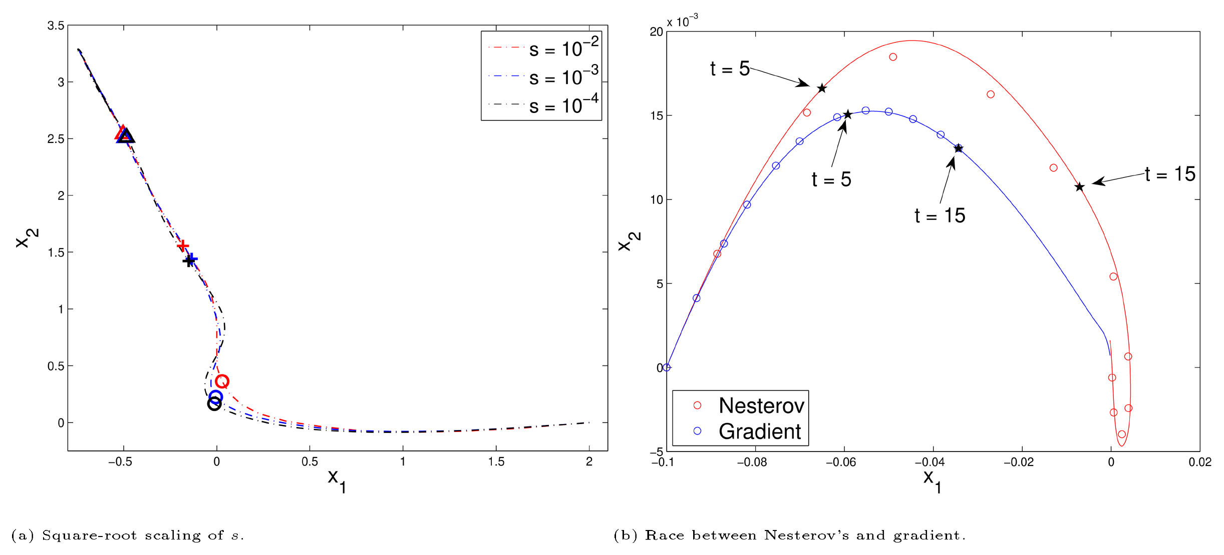
$**Figure 3:** In (a), the circles, crosses and triangles are $x_k$ evaluated at $k = \left\lceil 1/\sqrt{s} \right\rceil, \left\lceil 2/\sqrt{s} \right\rceil$ and $\left\lceil 3/\sqrt{s} \right\rceil$, respectively. In (b), the circles are iterations given by Nesterov's scheme or gradient descent, depending on the color, and the stars are $X(t)$ on the integral curves for $t = 5, 15$.$

A second look at Figure 3b suggests that Nesterov's scheme allows a large deviation from its limit curve, as compared with gradient descent. This raises the question of the stable step size allowed for numerically solving the ODE Equation 3 in the presence of accumulated errors. The finite difference approximation by the forward Euler method is

$ \frac{X(t+\Delta t) -2X(t) + X(t-\Delta t)}{\Delta t^2} + \frac{3}{t}\frac{X(t) - X(t-\Delta t)}{\Delta t} + \nabla f(X(t)) = 0, $

which is equivalent to

$ X(t+\Delta t) = \Big(2 - \frac{3 \Delta t}{t}\Big)X(t) - \Delta t^2 \nabla f(X(t)) - \Big(1 - \frac{3 \Delta t}{t}\Big) X(t-\Delta t). $

Assuming $f$ is sufficiently smooth, we have $\nabla f(x + \delta x) \approx \nabla f(x) + \nabla^2f(x) \delta x$ for small perturbations $\delta x$, where $\nabla^2f(x)$ is the Hessian of $f$ evaluated at $x$. Identifying $k = t/\Delta t$, the characteristic equation of this finite difference scheme is approximately

$ \det \left(\lambda^2 - \left( 2 - \Delta t^2 \nabla^2f -\frac{3 \Delta t}{t}\right) \lambda + 1 - \frac{3 \Delta t}{t} \right)= 0. $

The numerical stability of Equation 22 with respect to accumulated errors is equivalent to this: all the roots of Equation 24 lie in the unit circle (see e.g. [27]). When $\nabla^2f \preceq L I_n$ (i.e. $LI_n - \nabla^2 f$ is positive semidefinite), if $\Delta t/t$ small and $\Delta t < 2/\sqrt{L}$, we see that all the roots of Equation 24 lie in the unit circle. On the other hand, if $\Delta t > 2/\sqrt{L}$, Equation 24 can possibly have a root $\lambda$ outside the unit circle, causing numerical instability. Under our identification $s = \Delta t^2$, a step size of $s = 1/L$ in Nesterov's scheme Equation 1 is approximately equivalent to a step size of $\Delta t = 1/\sqrt{L}$ in the forward Euler method, which is stable for numerically integrating Equation 22.

As a comparison, note that the finite difference scheme of the ODE $\dot{X}(t) + \nabla f(X(t)) = 0$, which models gradient descent with updates $x_{k+1} = x_k - s\nabla f(x_k)$, has the characteristic equation $\det(\lambda - (1 - \Delta t \nabla^2 f)) = 0$. Thus, to guarantee $-I_n \preceq 1 - \Delta t \nabla^2 f \preceq I_n$ in worst case analysis, one can only choose $\Delta t \le 2/L$ for a fixed step size, which is much smaller than the step size $2/\sqrt{L}$ for Equation 22 when $\nabla f$ is very variable, i.e., $L$ is large.

4. The Magic Constant 3

Section Summary: The constant 3 in the original momentum term arises from a simple index difference and produces the specific friction coefficient that yields an O(1/k²) convergence rate. The section shows that any larger friction parameter r can be substituted in its place while preserving the same rate, both for a family of continuous damped oscillators and for corresponding discrete proximal-gradient schemes; the proofs rely on suitably adjusted energy functionals that remain nonincreasing. Below the threshold r = 3 the quadratic rate is lost in general, although the authors note that extra structure on the objective may restore it, highlighting an apparently sharp phase transition.

Recall that the constant 3 appearing in the coefficient of $\dot{X}$ in Equation 3 originates from $(k+2) - (k-1) = 3$. This number leads to the momentum coefficient in Equation 1 taking the form $(k-1)/(k+2) = 1 - 3/k + O(1/k^2)$. In this section, we demonstrate that 3 can be replaced by any larger number, while maintaining the $O(1/k^2)$ convergence rate. To begin with, let us consider the following ODE parameterized by a constant $r$:

$ \ddot{X} + \frac{r}{t}\dot{X} + \nabla f(X) = 0 $

with initial conditions $X(0) = x_0, \dot{X}(0) = 0$. The proof of Theorem 1, which seamlessly applies here, guarantees the existence and uniqueness of the solution $X$ to this ODE.

Interpreting the damping ratio $r/t$ as a measure of friction[^3] in the damping system, our results say that more friction does not end the $O(1/t^2)$ and $O(1/k^2)$ convergence rate. On the other hand, in the lower friction setting, where $r$ is smaller than 3, we can no longer expect inverse quadratic convergence rate, unless some additional structures of $f$ are imposed. We believe that this striking phase transition at 3 deserves more attention as an interesting research challenge.

[^3]: In physics and engineering, damping may be modeled as a force proportional to velocity but opposite in direction, i.e. resisting motion; for instance, this force may be used as an approximation to the friction caused by drag. In our model, this force would be proportional to $-\frac{r}{t} \dot{X}$ where $\dot{X}$ is velocity and $\frac{r}{t}$ is the damping coefficient.

4.1 High Friction

Here, we study the convergence rate of Equation 25 with $r > 3$ and $f \in \mathcal{F}_{\infty}$. Compared with Equation 3, this new ODE as a damping suffers from higher friction. Following the strategy adopted in the proof of Theorem 3, we consider a new energy functional defined as

$ \nonumber \mathcal{E}(t) = \frac{2t^2}{r-1}(f(X(t)) - f^\star) + (r-1)\left|X(t) + \frac{t}{r-1}\dot{X(t)} - x^\star\right|^2. $

By studying the derivative of this functional, we get the following result.

########## {caption="Theorem 5"}

The solution $X$ to 25 satisfies

$ \nonumber f(X(t)) - f^\star \le \frac{(r-1)^2|x_0 - x^\star|^2}{2t^2}, \quad \int^{\infty}_0 t(f(X(t))-f^\star){\mathrm{d}} t \le \frac{(r-1)^2|x_0 - x^\star|^2}{2(r-3)}. $

Proof: Noting $r\dot{X} + t\ddot{X} = -t\nabla f(X)$, we get $\dot{\mathcal{E}}$ equal to

$ \begin{split} \frac{4t}{r-1}(f(X) - f^\star) + \frac{2t^2}{r-1}\langle \nabla f, \dot{X} \rangle

2\langle X + \frac{t}{r-1}\dot{X} - x^\star, r\dot{X} + t\ddot{X} \rangle\ = \frac{4t}{r-1}(f(X) - f^\star) - 2t\langle X - x^\star, \nabla f(X) \rangle \le -\frac{2(r-3)t}{r-1}(f(X) - f^\star), \end{split} $

where the inequality follows from the convexity of $f$. Since $f(X)\geq f^\star$, the last display implies that $\mathcal{E}$ is non-increasing. Hence

$ \nonumber \frac{2t^2}{r-1}(f(X(t)) - f^\star) \le \mathcal{E}(t) \le \mathcal{E}(0) = (r-1)|x_0 - x^\star|^2, $

yielding the first inequality of this theorem. To complete the proof, from Equation 28 it follows that

$ \nonumber \int^{\infty}_0\frac{2(r-3)t}{r-1}(f(X) - f^\star){\mathrm{d}} t \le -\int^{\infty}_0 \frac{{\mathrm{d}}\mathcal{E}}{{\mathrm{d}} t}{\mathrm{d}} t = \mathcal{E}(0) - \mathcal{E}(\infty) \le (r-1)|x_0 - x^\star|^2, $

as desired for establishing the second inequality.

The first inequality is the same as Equation 10 for the ODE Equation 3, except for a larger constant $(r-1)^2/2$. The second inequality measures the error $f(X(t)) - f^\star$ in an average sense, and cannot be deduced from the first inequality.

Now, it is tempting to obtain such analogs for the discrete Nesterov's scheme as well. Following the formulation of [13], we wish to minimize $f$ in the composite form $f(x) = g(x) + h(x)$, where $g\in\mathcal{F}_L$ for some $L>0$ and $h$ is convex on $\mathbb{R}^n$ possibly assuming extended value $\infty$. Define the proximal subgradient

$ \nonumber G_s(x) \triangleq \frac{x - \text{argmin}_{z}\left( |z - (x-s\nabla g(x))|^2/(2s) + h(z) \right) }{s}. $

Parametrizing by a constant $r$, we propose the generalized Nesterov's scheme,

$ \begin{gathered} \begin{aligned} &x_k = y_{k-1} - sG_s(y_{k-1})\ &y_k = x_k + \frac{k-1}{k+r-1}(x_k -x_{k-1}), \end{aligned} \end{gathered} $

starting from $y_0 = x_0$. The discrete analog of Theorem 5 is below.

########## {caption="Theorem 6"}

The sequence ${x_k}$ given by Equation 32 with $0 < s \le 1/L$ satisfies

$ \nonumber f(x_k) - f^\star \le \frac{(r-1)^2|x_0 - x^\star|^2}{2s(k+r-2)^2}, \quad \sum_{k=1}^{\infty}(k+r-1)(f(x_k)-f^\star) \le \frac{(r-1)^2|x_0-x^\star|^2}{2s(r-3)}. $

The first inequality suggests that the generalized Nesterov's schemes still achieve $O(1/k^2)$ convergence rate. However, if the error bound satisfies $f(x_{k'}) - f^\star \geq c/k'^2$ for some arbitrarily small $c > 0$ and a dense subsequence ${k'}$, i.e., $|{k'}\cap {1, \ldots, m}| \geq \alpha m$ for all $m \ge 1$ and some $\alpha > 0$, then the second inequality of the theorem would be violated. To see this, note that if it were the case, we would have $(k'+r-1)(f(x_{k'})-f^\star) \gtrsim \frac1{k'}$; the sum of the harmonic series $\frac1{k'}$ over a dense subset of ${1, 2, \ldots}$ is infinite. Hence, the second inequality is not trivial because it implies the error bound is, in some sense, $O(1/k^2)$ suboptimal.

Now we turn to the proof of this theorem. It is worth pointing out that, though based on the same idea, the proof below is much more complicated than that of Theorem 5.

Proof: Consider the discrete energy functional,

$ \nonumber \mathcal{E}(k) = \frac{2(k+r-2)^2s}{r-1}(f(x_k)-f^\star) + (r-1)|z_k - x^\star|^2, $

where $z_k = (k+r-1)y_k/(r-1) - kx_k/(r-1)$. If we have

$ \mathcal{E}(k) + \frac{2s[(r-3)(k+r-2)+1]}{r-1}(f(x_{k-1})-f^\star) \le \mathcal{E}(k-1), $

then it would immediately yield the desired results by summing Equation 35 over $k$. That is, by recursively applying Equation 35, we see

$ \begin{split} \nonumber \mathcal{E}(k) + \sum_{i=1}^k\frac{2s[(r-3)(i+r-2)+1]}{r-1}(f(x_{i-1})-f^\star) \ \le \mathcal{E}(0) = \frac{2(r-2)^2s}{r-1}(f(x_0)-f^\star) + (r-1)|x_0 - x^\star|^2, \end{split} $

which is equivalent to

$ \mathcal{E}(k) + \sum_{i=1}^{k-1}\frac{2s[(r-3)(i+r-1)+1]}{r-1}(f(x_{i})-f^\star) \le (r-1)|x_0 - x^\star|^2. $

Noting that the left-hand side of Equation 36 is lower bounded by $2s(k+r-2)^2(f(x_k)-f^\star)/(r-1)$, we thus obtain the first inequality of the theorem. Since $\mathcal{E}(k)\geq 0$, the second inequality is verified via taking the limit $k \rightarrow\infty$ in Equation 36 and replacing $(r-3)(i+r-1)+1$ by $(r-3)(i+r-1)$.

We now establish Equation 35. For $s\le 1/L$, we have the basic inequality,

$ f(y-sG_s(y)) \le f(x) + G_s(y)^T(y-x) - \frac{s}{2}|G_s(y)|^2, $

for any $x$ and $y$. Note that $y_{k-1}-sG_s(y_{k-1})$ actually coincides with $x_k$. Summing of $(k-1)/(k+r-2)\times(\text{eq:prox_ineq})$ with $x=x_{k-1}, y = y_{k-1}$ and $(r-1)/(k+r-2)\times(\text{eq:prox_ineq})$ with $x=x^\star, y=y_{k-1}$ gives

$ \nonumber \begin{aligned}f(x_k) &\le \frac{k-1}{k+r-2}f(x_{k-1}) + \frac{r-1}{k+r-2}f^\star\& + \frac{r-1}{k+r-2}G_s(y_{k-1})^T\Big(\frac{k+r-2}{r-1}y_{k-1}-\frac{k-1}{r-1}x_{k-1} - x^\star\Big) - \frac{s}{2}|G_s(y_{k-1})|^2\&= \frac{k-1}{k+r-2}f(x_{k-1}) + \frac{r-1}{k+r-2}f^\star + \frac{(r-1)^2}{2s(k+r-2)^2}\Big(|z_{k-1}-x^\star|^2 - |z_{k}-x^\star|^2\Big),\end{aligned} $

where we use $z_{k-1}-s(k+r-2)G_s(y_{k-1})/(r-1)=z_{k}$. Rearranging the above inequality and multiplying by $2s(k+r-2)^2/(r-1)$ gives the desired Equation 35.

In closing, we would like to point out this new scheme is equivalent to setting $\theta_k = (r-1)/(k+r-1)$ and letting $\theta_k(\theta_{k-1}^{-1} - 1)$ replace the momentum coefficient $(k-1)/(k+r-1)$. Then, the equal sign

quot;="$ in the update $\theta_{k+1} = (\sqrt{\theta_k^4 + 4\theta_k^2} - \theta_k^2 )/2$ has to be replaced by an inequality sign

quot;\ge"$. In examining the proof of Theorem 1(b) in [28], we can get an alternative proof of Theorem 6.

4.2 Low Friction

Now we turn to the case $r < 3$. Then, unfortunately, the energy functional approach for proving Theorem 5 is no longer valid, since the left-hand side of Equation 28 is positive in general. In fact, there are counterexamples that fail the desired $O(1/t^2)$ or $O(1/k^2)$ convergence rate. We present such examples in continuous time. Equally, these examples would also violate the $O(1/k^2)$ convergence rate in the discrete schemes, and we forego the details.

Let $f(x) = \frac12|x|^2$ and $X$ be the solution to 25. Then, $Y = t^{\frac{r-1}{2}}X$ satisfies

$ \nonumber t^2\ddot{Y} + t\dot{Y} + (t^2 - (r-1)^2/4)Y = 0. $

With the initial condition $Y(t) \approx t^{\frac{r-1}{2}}x_0$ for small $t$, the solution to the above Bessel equation in a vector form of order $(r-1)/2$ is $Y(t) = 2^{\frac{r-1}{2}}\Gamma((r+1)/2)J_{(r-1)/2}(t)x_0$. Thus,

$ \nonumber X(t) = \frac{2^{\frac{r-1}{2}}\Gamma((r+1)/2)J_{(r-1)/2}(t)}{t^{\frac{r-1}{2}}}x_0. $

For large $t$, the Bessel function $J_{(r-1)/2}(t) = \sqrt{2/(\pi t)}\big( \cos(t-(r-1)\pi/4-\pi/4) + O(1/t) \big)$. Hence,

$ \nonumber f(X(t)) - f^\star = O\left( |x_0 - x^\star|^2/t^r \right), $

where the exponent $r$ is tight. This rules out the possibility of inverse quadratic convergence of the generalized ODE and scheme for all $f \in \mathcal{F}_L$ if $r < 2$. An example with $r = 1$ is plotted in Figure 2.

Next, we consider the case $2 \le r < 3$ and let $f(x) = |x|$ (this also applies to multivariate $f = |x|$).[^4] Starting from $x_0 > 0$, we get $X(t) = x_0 - \frac{t^2}{2(1+r)}$ for $t \le \sqrt{2(1+r)x_0}$. Requiring continuity of $X$ and $\dot{X}$ at the change point 0, we get

$ X(t) = \frac{t^2}{2(1+r)} + \frac{2(2(1+r)x_0)^{\frac{r+1}{2}}}{(r^2-1)t^{r-1}} - \frac{r+3}{r-1}x_0 $

[^4]: This function does not have a Lipschitz continuous gradient. However, a similar pattern as in Figure 2 can be also observed if we smooth $|x|$ at an arbitrarily small vicinity of 0.

for $\sqrt{2(1+r)x_0} < t \le \sqrt{2c^\star(1+r)x_0}$, where $c^\star$ is the positive root other than 1 of $(r-1)c + 4c^{-\frac{r-1}{2}} = r+3$. Repeating this process solves for $X$. Note that $t^{1-r}$ is in the null space of $\ddot{X} + r\dot{X}/t$ and satisfies $t^2 \times t^{1-r} \rightarrow \infty$ as $t \rightarrow \infty$. For illustration, Figure 4 plots $t^2(f(X(t)) - f^\star)$ and $sk^2(f(x_k) - f^\star)$ with $r = 2, 2.5$, and $r = 4$ for comparison[^5]. It is clearly that inverse quadratic convergence does not hold for $r = 2, 2.5$, that is, Equation 2 does not hold for $r < 3$. Interestingly, in Figure 4a and Figure 4d, the scaled errors at peaks grow linearly, whereas for $r = 2.5$, the growth rate, though positive as well, seems sublinear.

[^5]: For Figure 4d, Figure 4e and Figure 4f, if running generalized Nesterov's schemes with too many iterations (e.g. $10^5$), the deviations from the ODE will grow. Taking a sufficiently small $s$ can solve this issue.

$**Figure 4:** Scaled errors $t^2(f(X(t))-f^\star)$ and $sk^2(f(x_k)-f^\star)$ of generalized ODEs and schemes for minimizing $f = |x|$. In (d), the step size $s = 10^{-6}$, in (e), $s = 10^{-7}$, and in (f), $s = 10^{-6}$.$

However, if $f$ possesses some additional property, inverse quadratic convergence is still guaranteed, as stated below. In that theorem, $f$ is assumed to be a continuously differentiable convex function.

########## {caption="Theorem 7"}

Suppose $1 < r < 3$ and let $X$ be a solution to the ODE Equation 25. If $(f - f^\star)^{\frac{r-1}{2}}$ is also convex, then

$ \nonumber f(X(t)) - f^\star \le \frac{(r-1)^2|x_0 - x^\star|^2}{2t^2}. $

Proof: Since $(f - f^\star)^{\frac{r-1}{2}}$ is convex, we obtain

$ \left( f(X(t)) - f^\star \right)^{\frac{r-1}{2}} \le \langle X - x^\star, \nabla(f(X) - f^\star)^{\frac{r-1}{2}} \rangle = \frac{r-1}{2}(f(X) - f^\star)^{\frac{r-3}{2}}\langle X - x^\star, \nabla f(X)\rangle, $

which can be simplified to $\frac{2}{r-1}(f(X) - f^\star) \le \langle X - x^\star, \nabla f(X)\rangle$. This inequality combined with Equation 28 leads to the monotonically decreasing of $\mathcal{E}(t)$ defined for Theorem 5. This completes the proof by noting $f(X)-f^\star\le (r-1)\mathcal{E}(t)/(2t^2)\le (r-1)\mathcal{E}(0)/(2t^2) = (r-1)^2|x_0 - x^\star|^2/(2t^2)$.

4.3 Strongly Convex $f$

Strong convexity is a desirable property for optimization. Making use of this property carefully suggests a generalized Nesterov's scheme that achieves optimal linear convergence ([9]). In that case, even vanilla gradient descent has a linear convergence rate. Unfortunately, the example given in the previous subsection simply rules out such possibility for Equation 1 and its generalizations Equation 32. However, from a different perspective, this example suggests that $O(t^{-r})$ convergence rate can be expected for Equation 25. In the next theorem, we prove a slightly weaker statement of this kind, that is, a provable $O(t^{-\frac{2r}{3}})$ convergence rate is established for strongly convex functions. Bridging this gap may require new tools and more careful analysis.

Let $f\in\mathcal{S}_{\mu,L}(\mathbb{R}^n)$ and consider a new energy functional for $\alpha > 2$ defined as

$ \nonumber \mathcal{E}(t; \alpha) = t^{\alpha}(f(X(t)) - f^\star) + \frac{(2r-\alpha)^2t^{\alpha-2}}{8}\Big|X(t) + \frac{2t}{2r-\alpha}\dot{X} - x^\star\Big|^2. $

When clear from the context, $\mathcal{E}(t; \alpha)$ is simply denoted as $\mathcal{E}(t)$. For $r > 3$, taking $\alpha = 2r/3$ in the theorem stated below gives $f(X(t)) - f^\star \lesssim |x_0 -x^\star|^2/t^{\frac{2r}{3}}$.

########## {caption="Theorem 8"}

For any $f\in\mathcal{S}_{\mu,L}(\mathbb{R}^n)$, if $2 \le \alpha \le 2r/3$ we get

$ \nonumber f(X(t)) - f^\star \le \frac{C|x_0-x^\star|^2}{\mu^{\frac{\alpha-2}{2}}t^{\alpha}} $

for any $t > 0$. Above, the constant $C$ only depends on $\alpha$ and $r$.

Proof: Note that $\dot{\mathcal{E}}(t; \alpha)$ equals

$ \begin{split} \alpha t^{\alpha - 1}(f(X)-f^\star) - \frac{(2r-\alpha)t^{\alpha-1}}{2}\langle X- x^\star, \nabla f(X)\rangle + \frac{(\alpha-2)(2r-\alpha)^2t^{\alpha-3}}{8}|X-x^\star|^2 \+ \frac{(\alpha-2)(2r-\alpha)t^{\alpha-2}}{4}\langle \dot{X}, X - x^\star\rangle. \end{split} $

By the strong convexity of $f$, the second term of the right-hand side of Equation 45 is bounded below as

$ \nonumber \begin{aligned} \frac{(2r-\alpha)t^{\alpha-1}}{2}\langle X- x^\star, \nabla f(X)\rangle \geq \frac{(2r-\alpha)t^{\alpha-1}}{2}(f(X) -f^\star) + \frac{\mu(2r-\alpha)t^{\alpha-1}}{4}|X-x^\star|^2. \end{aligned} $

Substituting the last display into Equation 45 with the awareness of $r \geq 3\alpha/2$ yields

$ \begin{split} \nonumber \dot{\mathcal{E}} \le - \frac{(2\mu(2r-\alpha)t^2 - (\alpha-2)(2r-\alpha)^2)t^{\alpha-3}}{8}|X-x^\star|^2 + \frac{(\alpha-2)(2r-\alpha)t^{\alpha-2}}{8}\frac{{\mathrm{d}}|X-x^\star|^2}{{\mathrm{d}} t}. \end{split} $

Hence, if $t \geq t_{\alpha} := \sqrt{(\alpha-2)(2r-\alpha)/(2\mu)}$, we obtain

$ \nonumber \dot{\mathcal{E}}(t) \le \frac{(\alpha-2)(2r-\alpha)t^{\alpha-2}}{8}\frac{{\mathrm{d}}|X-x^\star|^2}{{\mathrm{d}} t}. $

Integrating the last inequality on the interval $(t_{\alpha}, t)$ gives

$ \begin{split} \mathcal{E}(t) \le \mathcal{E}(t_{\alpha}) + \frac{(\alpha-2)(2r-\alpha)t^{\alpha-2}}{8}|X(t)-x^\star|^2 - \frac{(\alpha-2)(2r-\alpha)t_{\alpha}^{\alpha-2}}{8}|X(t_{\alpha})-x^\star|^2 \- \frac{1}{8}\int^t_{t_{\alpha}}(\alpha-2)^2(2r-\alpha)u^{\alpha-3}|X(u)-x^\star|^2 {\mathrm{d}} u \le \mathcal{E}(t_{\alpha}) + \frac{(\alpha-2)(2r-\alpha)t^{\alpha-2}}{8}|X(t)-x^\star|^2\ \le \mathcal{E}(t_{\alpha}) + \frac{(\alpha-2)(2r-\alpha)t^{\alpha-2}}{4\mu}(f(X(t)) - f^\star). \end{split} $

Making use of Equation 48, we apply induction on $\alpha$ to finish the proof. First, consider $2 < \alpha \le 4$. Applying Theorem 5, from Equation 48 we get that $\mathcal{E}(t)$ is upper bounded by

$ \mathcal{E}(t_{\alpha}) + \frac{(\alpha-2)(r-1)^2(2r-\alpha)|x_0-x^\star|^2}{8\mu t^{4-\alpha}} \le \mathcal{E}(t_{\alpha}) + \frac{(\alpha-2)(r-1)^2(2r-\alpha)|x_0-x^\star|^2}{8\mu t_{\alpha}^{4-\alpha}}. $

Then, we bound $\mathcal{E}(t_{\alpha})$ as follows.

$ \begin{split} \mathcal{E}(t_{\alpha}) \le t_{\alpha}^{\alpha}(f(X(t_{\alpha})) - f^\star) + \frac{(2r-\alpha)^2t_{\alpha}^{\alpha-2}}{4}\Big|\frac{2r-2}{2r-\alpha}X(t_{\alpha})+ \frac{2t_{\alpha}}{2r-\alpha}\dot{X}(t_{\alpha}) - \frac{2r-2}{2r-\alpha}x^\star\Big|^2\

\frac{(2r-\alpha)^2t_{\alpha}^{\alpha-2}}{4}\Big|\frac{\alpha-2}{2r-\alpha}X(t_{\alpha}) - \frac{\alpha-2}{2r-\alpha}x^\star\Big|^2 \ \le (r-1)^2t_{\alpha}^{\alpha-2}|x_0-x^\star|^2 + \frac{(\alpha-2)^2(r-1)^2|x_0-x^\star|^2}{4\mu t_{\alpha}^{4-\alpha}}, \end{split} $

where in the second inequality we use the decreasing property of the energy functional defined for Theorem 5. Combining Equation 49 and 50, we have

$ \nonumber \mathcal{E}(t) \le (r-1)^2t_{\alpha}^{\alpha-2}|x_0-x^\star|^2 + \frac{(\alpha-2)(r-1)^2(2r+\alpha-4)|x_0-x^\star|^2}{8\mu t_{\alpha}^{4-\alpha}} = O \Big( \frac{|x_0-x^\star|^2}{\mu^{\frac{\alpha-2}{2}}} \Big). $

For $t \ge t_{\alpha}$, it suffices to apply $f(X(t))-f^\star\le \mathcal{E}(t)/t^3$ to the last display. For $t < t_{\alpha}$, by Theorem 5, $f(X(t)) - f^\star$ is upper bounded by

$ \begin{aligned} \frac{(r-1)^2|x_0 - x^\star|^2}{2t^2} &\le \frac{(r-1)^2\mu^{\frac{\alpha-2}{2}}[(\alpha-2)(2r-\alpha)/(2\mu)]^{\frac{\alpha-2}{2}}}{2}\frac{|x_0-x^\star|^2}{\mu^{\frac{\alpha-2}{2}}t^{\alpha}} \ &= O\Big(\frac{|x_0-x^\star|^2}{\mu^{\frac{\alpha-2}{2}}t^{\alpha}} \Big). \end{aligned} $

Next, suppose that the theorem is valid for some $\tilde{\alpha} > 2$. We show below that this theorem is still valid for $\alpha := \tilde{\alpha} + 1$ if still $r \geq 3\alpha/2$. By the assumption, Equation 48 further induces

$ \nonumber \mathcal{E}(t) \le \mathcal{E}(t_{\alpha}) + \frac{(\alpha-2)(2r-\alpha)t^{\alpha-2}}{4\mu}\frac{\tilde{C}|x_0 - x^\star|^2}{\mu^{\frac{\tilde{\alpha}-2}{2}}t^{\tilde{\alpha}}} \le \mathcal{E}(t_{\alpha}) + \frac{\tilde{C}(\alpha-2)(2r-\alpha)|x_0 - x^\star|^2}{4\mu^{\frac{\alpha-1}{2}}t_{\alpha}} $

for some constant $\tilde{C}$ only depending on $\tilde{\alpha}$ and $r$. This inequality with Equation 50 implies

$ \begin{aligned} \nonumber \mathcal{E}(t) &\le (r-1)^2t_{\alpha}^{\alpha-2}|x_0-x^\star|^2 + \frac{(\alpha-2)^2(r-1)^2|x_0-x^\star|^2}{4\mu t_{\alpha}^{4-\alpha}} + \frac{\tilde{C}(\alpha-2)(2r-\alpha)|x_0 - x^\star|^2}{4\mu^{\frac{\alpha-1}{2}}t_{\alpha}} \ &= O\left( |x_0-x^\star|^2/\mu^{\frac{\alpha-2}{2}} \right), \end{aligned} $

which verify the induction for $t \geq t_{\alpha}$. As for $t < t_{\alpha}$, the validity of the induction follows from Theorem 5, similarly to 52. Thus, combining the base and induction steps, the proof is completed.

It should be pointed out that the constant $C$ in the statement of Theorem 8 grows with the parameter $r$. Hence, simply increasing $r$ does not guarantee to give a better error bound. While it is desirable to expect a discrete analogy of Theorem 8, i.e., $O(1/k^{\alpha})$ convergence rate for Equation 32, a complete proof can be notoriously complicated. That said, we mimic the proof of Theorem 8 for $\alpha = 3$ and succeed in obtaining a $O(1/k^3)$ convergence rate for the generalized Nesterov's schemes, as summarized in the theorem below.

########## {caption="Theorem 9"}

Suppose $f$ is written as $f = g + h$, where $g\in\mathcal{S}_{\mu,L}$ and $h$ is convex with possible extended value $\infty$. Then, the generalized Nesterov's scheme Equation 32 with $r\geq 9/2$ and $s = 1/L$ satisfies

$ \nonumber f(x_k) - f^\star \le \frac{CL|x_0-x^\star|^2}{k^2}\frac{\sqrt{L/\mu}}{k}, $

where $C$ only depends on $r$.

This theorem states that the discrete scheme Equation 32 enjoys the error bound $O(1/k^3)$ without any knowledge of the condition number $L/\mu$. In particular, this bound is much better than that given in Theorem 6 if $k \gg \sqrt{L/\mu}$. The strategy of the proof is fully inspired by that of Theorem 8, though it is much more complicated and thus deferred to the Appendix. The relevant energy functional $\mathcal{E}(k)$ for this Theorem 9 is equal to

$ \begin{split} \frac{s(2k+3r-5)(2k+2r-5)(4k+4r-9)}{16}(f(x_k)-f^\star)\ + \frac{2k+3r-5}{16}|2(k+r-1)y_k - (2k+1)x_k - (2r-3)x^\star|^2. \end{split} $

4.4 Numerical Examples

We study six synthetic examples to compare Equation 32 with the step sizes are fixed to be $1/L$, as illustrated in Figure 5. The error rates exhibits similar patterns for all $r$, namely, decreasing while suffering from local bumps. A smaller $r$ introduces less friction, thus allowing $x_k$ moves towards $x^\star$ faster in the beginning. However, when sufficiently close to $x^\star$, more friction is preferred in order to reduce overshoot. This point of view explains what we observe in these examples. That is, across these six examples, Equation 32 with a smaller $r$ performs slightly better in the beginning, but a larger $r$ has advantage when $k$ is large. It is an interesting question how to choose a good $r$ for different problems in practice.

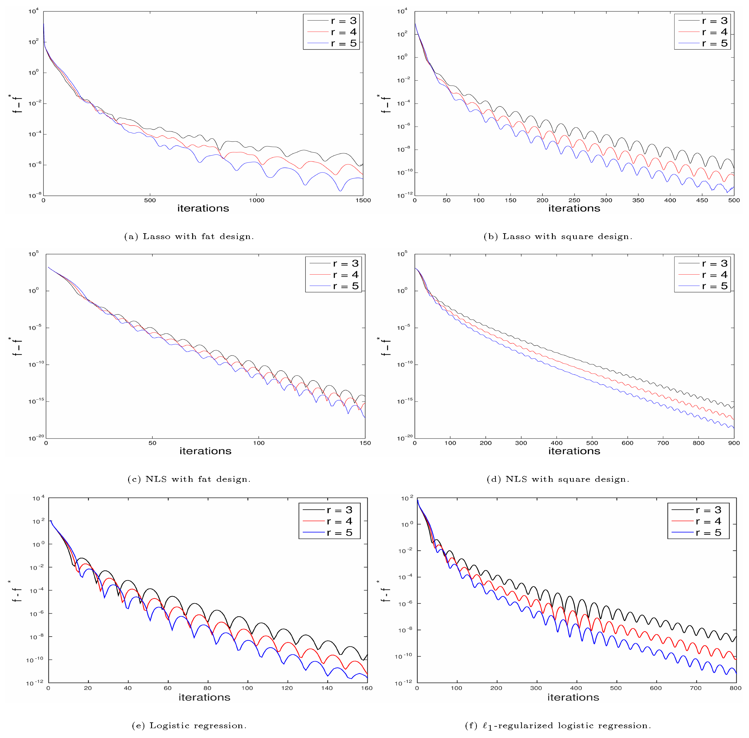
**Figure 5:** Comparisons of generalized Nesterov's schemes with different $r$.

Lasso with fat design. Minimize $f(x) = \frac{1}{2}|Ax-b|^2 + \lambda|x|_1$, in which $A$ a $100\times 500$ random matrix with i.i.d. standard Gaussian $\mathcal{N}(0, 1)$ entries, $b$ generated independently has i.i.d. $\mathcal{N}(0, 25)$ entries, and the penalty $\lambda = 4$. The plot is Figure 5a.

Lasso with square design. Minimize $f(x) = \frac{1}{2}|Ax-b|^2 + \lambda|x|_1$, where $A$ a $500\times 500$ random matrix with i.i.d. standard Gaussian entries, $b$ generated independently has i.i.d. $\mathcal{N}(0, 9)$ entries, and the penalty $\lambda = 4$. The plot is Figure 5b.

Nonnegative least squares (NLS) with fat design. Minimize $f(x) = |Ax-b|^2$ subject to $x\succeq 0$, with the same design $A$ and $b$ as in Figure 5a. The plot is Figure 5c.

Nonnegative least squares with sparse design. Minimize $f(x) = |Ax-b|^2$ subject to $x\succeq 0$, in which $A$ is a $1000\times 10000$ sparse matrix with nonzero probability $10%$ for each entry and $b$ is given as $b = Ax^0 + \mathcal{N}(0, I_{1000})$. The nonzero entries of $A$ are independently Gaussian distributed before column normalization, and $x^0$ has 100 nonzero entries that are all equal to 4. The plot is Figure 5d.

Logistic regression. Minimize $\sum_{i=1}^n - y_i a_i^T x + \log(1 + \mathrm{e}^{a_i^T x})$, in which $A = (a_1, \ldots, a_n)^T$ is a $500 \times 100$ matrix with i.i.d. $\mathcal{N}(0,1)$ entries. The labels $y_i \in {0, 1}$ are generated by the logistic model: $\mathbb{P}(Y_i = 1) = 1/(1 + \mathrm{e}^{-a_i^T x^0})$, where $x^0$ is a realization of i.i.d. $\mathcal{N}(0, 1/100)$. The plot is Figure 5e.

$\ell_1$-regularized logistic regression. Minimize $\sum_{i=1}^n - y_i a_i^T x + \log(1 + \mathrm{e}^{a_i^T x}) + \lambda |x|_1$, in which $A = (a_1, \ldots, a_n)^T$ is a $200 \times 1000$ matrix with i.i.d. $\mathcal{N}(0,1)$ entries and $\lambda = 5$. The labels $y_i$ are generated similarly as in the previous example, except for the ground truth $x^0$ here having 10 nonzero components given as i.i.d. $\mathcal{N}(0, 225)$. The plot is Figure 5f.

5. Restarting

Section Summary: The section explains that Nesterov's accelerated method and its generalizations cannot fully exploit strong convexity, because excessive momentum produces overshooting and prevents the linear convergence rate that even the plain gradient method achieves. It therefore introduces a speed-restarting procedure that resets the momentum coefficient each time velocity begins to drop, keeping the trajectory from losing friction in the associated differential equation. The resulting restarted flow is proved to converge linearly, with the function-value error decaying exponentially at a rate that depends only on the condition number.

The example discussed in Section 4.2 demonstrates that Nesterov's scheme and its generalizations Equation 32 are not capable of fully exploiting strong convexity. That is, this example suggests evidence that $O(1/\mathtt{poly}(k))$ is the best rate achievable under strong convexity. In contrast, the vanilla gradient method achieves linear convergence $O((1-\mu/L)^k)$. This drawback results from too much momentum introduced when the objective function is strongly convex. The derivative of a strongly convex function is generally more reliable than that of non-strongly convex functions. In the language of ODEs, at later stage a too small $3/t$ in Equation 3 leads to a lack of friction, resulting in unnecessary overshoot along the trajectory. Incorporating the optimal momentum coefficient $\frac{\sqrt{L} - \sqrt{\mu}}{\sqrt{L} + \sqrt{\mu}}$ (This is less than $(k-1)/(k+2)$ when $k$ is large), Nesterov's scheme has convergence rate of $O((1-\sqrt{\mu/L})^k)$ ([9]), which, however, requires knowledge of the condition number $\mu/L$. While it is relatively easy to bound the Lipschitz constant $L$ by the use of backtracking, estimating the strong convexity parameter $\mu$, if not impossible, is very challenging.

Among many approaches to gain acceleration via adaptively estimating $\mu/L$ (see [11]), [24] proposes a procedure termed as gradient restarting for Nesterov's scheme in which Equation 1 is restarted with $x_0 = y_0 :=x_k$ whenever $f(x_{k+1}) > f(x_k)$. In the language of ODEs, this restarting essentially keeps $\langle \nabla f,\dot{X} \rangle$ negative, and resets $3/t$ each time to prevent this coefficient from steadily decreasing along the trajectory. Although it has been empirically observed that this method significantly boosts convergence, there is no general theory characterizing the convergence rate.

In this section, we propose a new restarting scheme we call the speed restarting scheme. The underlying motivation is to maintain a relatively high velocity $\dot{X}$ along the trajectory, similar in spirit to the gradient restarting. Specifically, our main result, Theorem 10, ensures linear convergence of the continuous version of the speed restarting. More generally, our contribution here is merely to provide a framework for analyzing restarting schemes rather than competing with other schemes; it is beyond the scope of this paper to get optimal constants in these results. Throughout this section, we assume $f\in \mathcal{S}{\mu,L}$ for some $0 < \mu \le L$. Recall that function $f\in \mathcal{S}{\mu,L}$ if $f\in \mathcal{F}_{L}$ and $f(x) - \mu |x|^2/2$ is convex.

5.1 A New Restarting Scheme

We first define the speed restarting time. For the ODE Equation 3, we call

$ \nonumber T = T(x_0; f) = \sup \left{t > 0: \forall u\in (0, t), ~ \frac{{\mathrm{d}}|\dot{X}(u)|^2}{{\mathrm{d}} u} > 0 \right} $

the speed restarting time. In words, $T$ is the first time the velocity $|\dot{X}|$ decreases. Back to the discrete scheme, it is the first time when we observe $|x_{k+1} - x_k| < |x_k - x_{k-1}|$. This definition itself does not directly imply that $0 < T < \infty$, which is proven later in Lemma 13 and Lemma 24. Indeed, $f(X(t))$ is a decreasing function before time $T$; for $t\le T$,

$ \nonumber \frac{{\mathrm{d}} f(X(t))}{{\mathrm{d}} t} =\langle \nabla f(X),\dot{X}\rangle = -\frac{3}{t}|\dot{X}|^2 - \frac{1}{2}\frac{{\mathrm{d}}|\dot{X}|^2}{\mathrm{d} t} \le 0. $

The speed restarted ODE is thus

$ \ddot{X}(t) + \frac{3}{t_{\mathrm{sr}}}\dot{X}(t) + \nabla f(X(t)) = 0, $

where $t_{\mathrm{sr}}$ is set to zero whenever $\langle \dot{X}, \ddot{X}\rangle = 0$ and between two consecutive restarts, $t_{\mathrm{sr}}$ grows just as $t$. That is, $t_{\mathrm{sr}} = t - \tau$, where $\tau$ is the latest restart time. In particular, $t_{\mathrm{sr}} = 0$ at $t = 0$. Letting $X^{\mathrm{sr}}$ be the solution to 58, we have the following observations.

$X^{\mathrm{sr}}(t)$ is continuous for $t \geq 0$, with $X^{\mathrm{sr}}(0) = x_0$;
$X^{\mathrm{sr}}(t)$ satisfies Equation 3 for $0 < t < T_1 := T(x_0; f)$.
Recursively define $T_{i+1} = T\left( X^{\mathrm{sr}}\left(\sum_{j=1}^i T_j\right); f\right)$ for $i \ge 1$, and $\widetilde{X}(t) := X^{\mathrm{sr}}\left(\sum_{j=1}^i T_j + t \right)$ satisfies the ODE Equation 3, with $\widetilde{X}(0) = X^{\mathrm{sr}} \left( \sum_{j=1}^i T_j \right)$, for $0 < t < T_{i+1}$.

The theorem below guarantees linear convergence of $X^{\mathrm{sr}}$. This is a new result in the literature ([24, 29]). The proof of Theorem 10 is based on Lemma 12 and Lemma 13, where the first guarantees the rate $f(X^{\mathrm{sr}}) - f^\star$ decays by a constant factor for each restarting, and the second confirms that restartings are adequate. In these lemmas we all make a convention that the uninteresting case $x_0 = x^\star$ is excluded.

########## {caption="Theorem 10"}

There exist positive constants $c_1$ and $c_2$, which only depend on the condition number $L/\mu$, such that for any $f\in\mathcal{S}_{\mu, L}$, we have

$ \nonumber f(X^{\mathrm{sr}}(t)) - f^\star \le \frac{c_1L|x_0 - x^\star|^2}{2}\mathrm{e}^{-c_2t\sqrt{L}}. $

Before turning to the proof, we make a remark that this linear convergence of $X^{\mathrm{sr}}$ remains to hold for the generalized ODE Equation 25 with $r > 3$. Only minor modifications in the proof below are needed, such as replacing $u^3$ by $u^r$ in the definition of $I(t)$ in Lemma 24.

5.2 Proof of Linear Convergence

First, we collect some useful estimates. Denote by $M(t)$ the supremum of $|\dot{X}(u)|/{u}$ over $u\in (0, t]$ and let

$ I(t) := \int^t_0 u^3(\nabla f(X(u)) - \nabla f(x_0)) {\mathrm{d}} u. $

It is guaranteed that $M$ defined above is finite, for example, see the proof of Lemma 18. The definition of $M$ gives a bound on the gradient of $f$,

$ \nonumber |\nabla f(X(t)) - \nabla f(x_0)| \le L\Big|\int_{0}^t \dot{X}(u) {\mathrm{d}} u \Big| \le L\int_{0}^t u\frac{|\dot{X}(u)|}{u} {\mathrm{d}} u \le \frac{L M(t)t^2}{2}. $

Hence, it is easy to see that $I$ can also be bounded via $M$,

$ \nonumber |I(t)| \le \int_0^t u^3|\nabla f(X(u))-\nabla f(x_0)| {\mathrm{d}} u\le \int_0^t \frac{L M(u)u^5}{2}{\mathrm{d}} u\le \frac{LM(t)t^6}{12}. $

To fully facilitate these estimates, we need the following lemma that gives an upper bound of $M$, whose proof is deferred to the appendix.

########## {caption="Lemma 11"}

For $t < \sqrt{12/L}$, we have

$ \nonumber M(t) \le \frac{|\nabla f(x_0)|}{4(1 - Lt^2/12)}. $

Next we give a lemma which claims that the objective function decays by a constant through each speed restarting.

########## {caption="Lemma 12"}

There is a universal constant $C > 0$ such that

$ \nonumber f(X(T)) - f^\star \le \left( 1 - \frac{C\mu}{L} \right) (f(x_0) - f^\star). $

Proof: By Lemma 11, for $t < \sqrt{12/L}$ we have

$ \nonumber \left| \dot{X}(t) + \frac{t}{4}\nabla f(x_0) \right| = \frac{1}{t^3}|I(t)|\le \frac{LM(t)t^3}{12} \le \frac{L|\nabla f(x_0)|t^3}{48(1 - Lt^2/12)}, $

which yields

$ 0 \le \frac{t}{4}|\nabla f(x_0)| - \frac{L|\nabla f(x_0)|t^3}{48(1 - Lt^2/12)} \le |\dot{X}(t)| \le \frac{t}{4}|\nabla f(x_0)| + \frac{L|\nabla f(x_0)|t^3}{48(1 - Lt^2/12)}. $

Hence, for $0 < t < 4/(5\sqrt{L})$ we get

$ \begin{split} \nonumber \frac{{\mathrm{d}} f(X)}{{\mathrm{d}} t} = -\frac{3}{t}|\dot{X}|^2 - \frac{1}{2}\frac{{\mathrm{d}}}{{\mathrm{d}} t}|\dot{X}|^2 \le -\frac{3}{t}|\dot{X}|^2 \ \le -\frac{3}{t} \left(\frac{t}{4}|\nabla f(x_0)| - \frac{L|\nabla f(x_0)|t^3}{48(1 - Lt^2/12)}\right)^2 \le - C_1t|\nabla f(x_0)|^2, \end{split} $

where $C_1 > 0$ is an absolute constant and the second inequality follows from Lemma 24 in the appendix. Consequently,

$ f\left(X(4/(5\sqrt{L}))\right) - f(x_0) \le \int_{0}^{\frac{4}{5\sqrt{L}}}-C_1u|\nabla f(x_0)|^2 {\mathrm{d}} u \le -\frac{C\mu}{L}(f(x_0)-f^\star), $

where $C = 16C_1/25$ and in the last inequality we use the $\mu$-strong convexity of $f$. Thus we have

$ f\left( X \left(\frac{4}{5\sqrt{L}}\right)\right) - f^\star \le \left( 1 -\frac{C\mu}{L}\right)(f(x_0)-f^\star). $

To complete the proof, note that $f(X(T)) \le f(X(4/(5\sqrt{L})))$ by Lemma 24.

With each restarting reducing the error $f - f^\star$ by a constant a factor, we still need the following lemma to ensure sufficiently many restartings.

########## {caption="Lemma 13"}

There is a universal constant $\tilde{C}$ such that

$ T \le \frac{4\exp\left(\tilde{C} L/\mu\right)}{5\sqrt{L}}. $

Proof: For $4/(5\sqrt{L}) \le t \le T$, we have $\frac{{\mathrm{d}} f(X)}{{\mathrm{d}} t} \le -\frac{3}{t}|\dot{X}(t)|^2 \le -\frac{3}{t}|\dot{X}(4/(5\sqrt{L}))|^2$, which implies

$ f(X(T)) - f(x_0) \le -\int_{\frac{4}{5\sqrt{L}}}^T\frac{3}{t}|\dot{X}(4/(5\sqrt{L}))|^2 {\mathrm{d}} t = -3|\dot{X}(4/(5\sqrt{L}))|^2\log\frac{5T\sqrt{L}}{4}. $

Hence, we get an upper bound for $T$,

$ \nonumber T \le \frac{4}{5\sqrt{L}}\exp\Big(\frac{f(x_0) - f(X(T))}{3|\dot{X}(4/(5\sqrt{L}))|^2} \Big)\le \frac{4}{5\sqrt{L}}\exp\Big(\frac{f(x_0) - f^\star}{3|\dot{X}(4/(5\sqrt{L}))|^2} \Big). $

Plugging $t = 4/(5\sqrt{L})$ into Equation 65 gives $|\dot{X}(4/(5\sqrt{L}))| \geq \frac{C_1}{\sqrt{L}}|\nabla f(x_0)|$ for some universal constant $C_1 > 0$. Hence, from the last display we get

$ T \le\frac{4}{5\sqrt{L}}\exp\left( \frac{L(f(x_0)-f^\star)}{3C_1^2|\nabla f(x_0)|^2} \right) \le \frac{4}{5\sqrt{L}}\exp\frac{L}{6C_1^2\mu}. $

Now, we are ready to prove Theorem 10 by applying Lemma 12 and Lemma 13.

Proof: Note that Lemma 13 asserts, by time $t$ at least $m := \lfloor 5t\sqrt{L}\mathrm{e}^{-\tilde{C} L/\mu}/4\rfloor$ restartings have occurred for $X^{\mathrm{sr}}$. Hence, recursively applying Lemma 12, we have

$ \begin{aligned} f(X^{\mathrm{sr}}(t)) - f^\star &\le f \left( X^{\mathrm{sr}}(T_1 + \cdots + T_m) \right) - f^\star \ &\le (1 - C\mu/L) \left(f \left( X^{\mathrm{sr}}(T_1 + \cdots + T_{m-1}) \right) - f^\star \right)\ & \le \cdots \le \cdots \ &\le (1 - C\mu/L)^m (f(x_0) - f^\star) \le \mathrm{e}^{- C\mu m/L} (f(x_0) - f^\star) \ &\le c_1\mathrm{e}^{-c_2t\sqrt{L}}(f(x_0) - f^\star) \le \frac{c_1L|x_0 - x^\star|^2}{2}\mathrm{e}^{-c_2t\sqrt{L}}, \end{aligned} $

where $c_1 = \exp(C\mu/L)$ and $c_2 = 5C\mu e^{-\tilde{C} \mu/L}/(4L)$.

In closing, we remark that we believe that estimate in Lemma 12 is tight, while not for Lemma 13. Thus we conjecture that for a large class of $f\in\mathcal{S}_{\mu,L}$, if not all, $T = O(\sqrt{L}/\mu)$. If this is true, the exponent constant $c_2$ in Theorem 10 can be significantly improved.

5.3 Numerical Examples

Below we present a discrete analog to the restarted scheme. There, $k_{\min}$ is introduced to avoid having consecutive restarts that are too close. To compare the performance of the restarted scheme with the original Equation 1, we conduct four simulation studies, including both smooth and non-smooth objective functions. Note that the computational costs of the restarted and non-restarted schemes are the same.

input: $x_0\in \mathbb{R}^n, y_0 = x_0, x_{-1} = x_0, 0 < s \le 1/L, k_{\max}\in\mathbb{N}^+$ and $k_{\min}\in\mathbb{N}^+$
$j \gets 1$
for $k = 1$ to $k_{\max}$ do
  $x_k \gets \text{argmin}_x(\frac{1}{2s}\|x - y_{k-1} + s\nabla g(y_{k-1})\|^2 + h(x))$
  $y_k \gets x_k + \frac{j-1}{j+2}(x_k - x_{k-1})$
  if $\|x_k - x_{k-1}\| < \|x_{k-1} - x_{k-2}\|$ and $j \ge k_{\min}$ then
    $j \gets 1$
  else
    $j \gets j + 1$
  end if
end for

Quadratic. $f(x) = \frac{1}{2} x^TAx + b^Tx$ is a strongly convex function, in which $A$ is a $500\times 500$ random positive definite matrix and $b$ a random vector. The eigenvalues of $A$ are between $0.001$ and $1$. The vector $b$ is generated as i.i.d. Gaussian random variables with mean 0 and variance 25.

Log-sum-exp.

$ \nonumber f(x) = \rho\log\Big[\sum_{i=1}^m\exp((a_i^Tx - b_i)/\rho)\Big], $

where $n = 50, m = 200, \rho = 20$. The matrix $A = (a_{ij})$ is a random matrix with i.i.d. standard Gaussian entries, and $b = (b_i)$ has i.i.d. Gaussian entries with mean $0$ and variance $2$. This function is not strongly convex.

Matrix completion. $f(X) = \frac{1}{2} |X_{\mathrm{obs}} - M_{\mathrm{obs}}|F^2 + \lambda|X|*$, in which the ground truth $M$ is a rank-5 random matrix of size $300\times 300$. The regularization parameter is set to $\lambda = 0.05$. The 5 singular values of $M$ are $1, \ldots, 5$. The observed set is independently sampled among the $300\times 300$ entries so that 10% of the entries are actually observed.

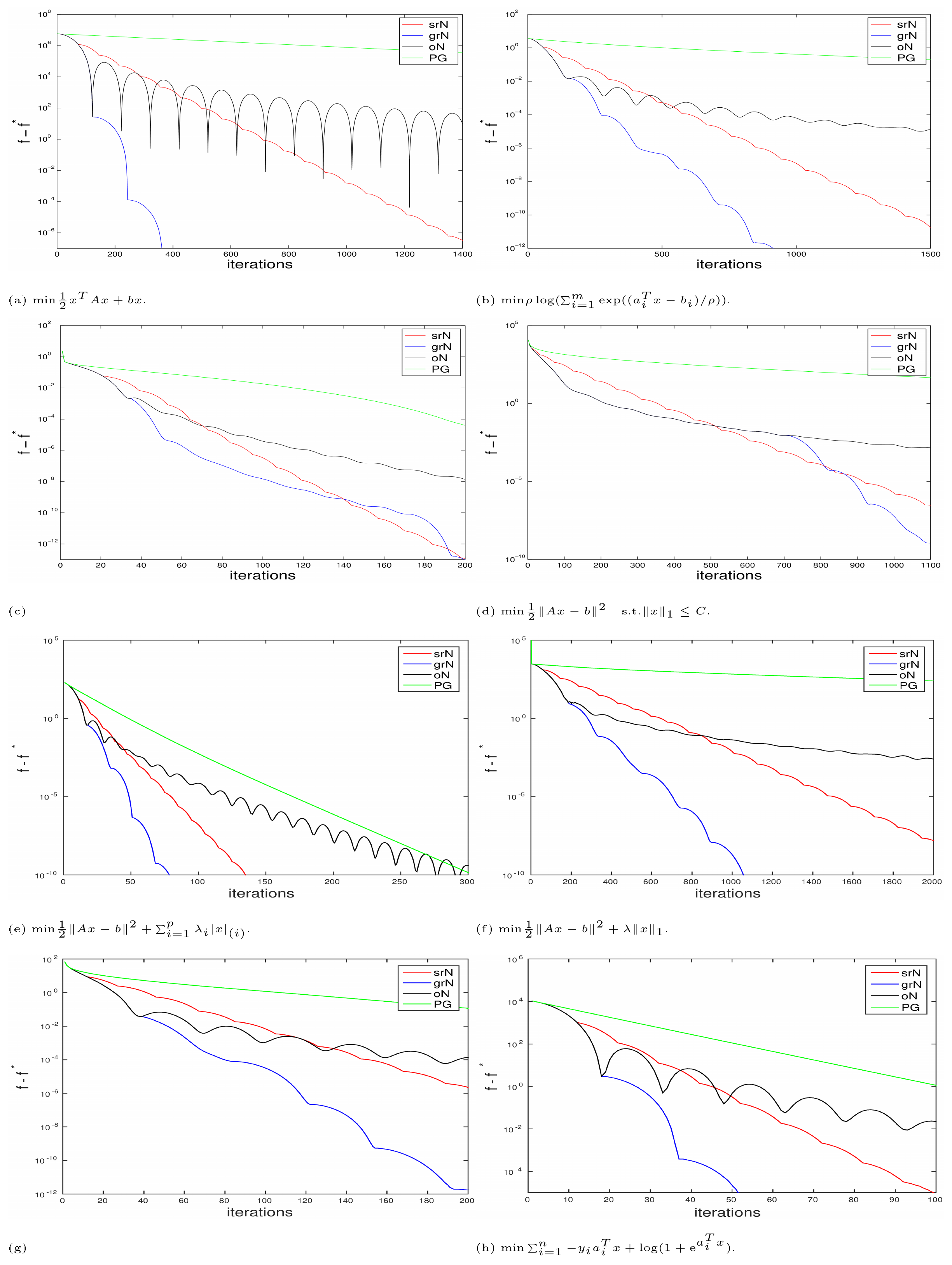
**Figure 6:** Numerical performance of speed restarting (srN), gradient restarting (grN), the original Nesterov's scheme (oN) and the proximal gradient (PG).

Lasso in $\ell_1$–constrained form with large sparse design. $f(x) = \frac{1}{2}|Ax-b|^2\quad \text{s.t.}~ |x|_1\le \delta$, where $A$ is a $5000\times 50000$ random sparse matrix with nonzero probability $0.5%$ for each entry and $b$ is generated as $b = Ax^0 + z$. The nonzero entries of $A$ independently follow the Gaussian distribution with mean 0 and variance $0.04$. The signal $x^0$ is a vector with 250 nonzeros and $z$ is i.i.d. standard Gaussian noise. The parameter $\delta$ is set to $|x^0|_1$.

Sorted $\ell_1$ penalized estimation. $f(x) = \frac{1}{2} |Ax - b|^2 + \sum_{i=1}^p \lambda_i |x|{(i)}$, where $|x|{(1)} \ge \cdots \ge |x|_{(p)}$ are the order statistics of $|x|$. This is a recently introduced testing and estimation procedure ([30]). The design $A$ is a $1000 \times 10000$ Gaussian random matrix, and $b$ is generated as $b = Ax^0 + z$ for 20-sparse $x^0$ and Gaussian noise $z$. The penalty sequence is set to $\lambda_i = 1.1\Phi^{-1}(1-0.05i/(2p))$.

Lasso. $f(x) = \frac{1}{2}|Ax-b|^2 + \lambda |x|_1$, where $A$ is a $1000\times 500$ random matrix and $b$ is given as $b = Ax^0 + z$ for 20-sparse $x^0$ and Gaussian noise $z$. We set $\lambda = 1.5\sqrt{2\log p}$.

$\ell_1$-regularized logistic regression. $f(x) = \sum_{i=1}^n - y_i a_i^T x + \log(1 + \mathrm{e}^{a_i^T x}) + \lambda |x|_1$, where the setting is the same as in Figure 5f. The results are presented in Figure 6g.

Logistic regression with large sparse design. $f(x) = \sum_{i=1}^n - y_i a_i^T x + \log(1 + \mathrm{e}^{a_i^T x})$, in which $A = (a_1, \ldots, a_n)^T$ is a $10^7 \times 20000$ sparse random matrix with nonzero probability $0.1%$ for each entry, so there are roughly $2 \times 10^8$ nonzero entries in total. To generate the labels $y$, we set $x^0$ to be i.i.d. $\mathcal{N}(0, 1/4)$. The plot is Figure 6h.

In these examples, $k_{\min}$ is set to be 10 and the step sizes are fixed to be $1/L$. If the objective is in composite form, the Lipschitz bound applies to the smooth part. Figure 6 presents the performance of the speed restarting scheme, the gradient restarting scheme, the original Nesterov's scheme and the proximal gradient method. The objective functions include strongly convex, non-strongly convex and non-smooth functions, violating the assumptions in Theorem 10. Among all the examples, it is interesting to note that both speed restarting scheme empirically exhibit linear convergence by significantly reducing bumps in the objective values. This leaves us an open problem of whether there exists provable linear convergence rate for the gradient restarting scheme as in Theorem 10. It is also worth pointing out that compared with gradient restarting, the speed restarting scheme empirically exhibits more stable linear convergence rate.

6. Discussion

Section Summary: This paper presents a continuous-time ODE framework for analyzing Nesterov's accelerated gradient method, which helps explain observed behaviors such as oscillations and leads to new generalized schemes that converge at the optimal O(1/k²) rate as well as a restarting strategy that achieves linear convergence for strongly convex functions. The authors note that translating insights from the ODE to practical discrete updates requires careful tuning, and they call for a general theory that would make this mapping more systematic. They also point out that viewing the ODE as a surrogate model opens the door to further algorithmic improvements, such as better step-size selection and stopping rules based on trajectory properties like curvature.

This paper introduces a second-order ODE and accompanying tools for characterizing Nesterov's accelerated gradient method. This ODE is applied to study variants of Nesterov's scheme and is capable of interpreting some empirically observed phenomena, such as oscillations along the trajectories. Our approach suggests (1) a large family of generalized Nesterov's schemes that are all guaranteed to converge at the rate $O(1/k^2)$, and (2) a restarting scheme provably achieving a linear convergence rate whenever $f$ is strongly convex.

In this paper, we often utilize ideas from continuous-time ODEs, and then apply these ideas to discrete schemes. The translation, however, involves parameter tuning and tedious calculations. This is the reason why a general theory mapping properties of ODEs into corresponding properties for discrete updates would be a welcome advance. Indeed, this would allow researchers to only study the simpler and more user-friendly ODEs.

As evidenced by many examples, the viewpoint of regarding the ODE as a surrogate for Nesterov's scheme would allow a new perspective for studying accelerated methods in optimization. The discrete scheme and the ODE are closely connected by the exact mapping between the coefficients of momentum (e.g. $(k-1)/(k+2)$) and velocity (e.g. $3/t$). The derivations of generalized Nesterov's schemes and the speed restarting scheme are both motivated by trying a different velocity coefficient, in which the surprising phase transition at 3 is observed. Clearly, such alternatives are endless, and we expect this will lead to findings of many discrete accelerated schemes. In a different direction, a better understanding of the trajectory of the ODEs, such as curvature, has the potential to be helpful in deriving appropriate stopping criteria for termination, and choosing step size by backtracking.

Acknowledgments W. S. was partially supported by a General Wang Yaowu Stanford Graduate Fellowship. S. B. was partially supported by DARPA XDATA. E. C. was partially supported by AFOSR under grant FA9550-09-1-0643, by NSF under grant CCF-0963835, and by the Math + X Award from the Simons Foundation. We would like to thank Carlos Sing-Long, Zhou Fan, and Xi Chen for helpful discussions about parts of this paper. We would also like to thank the associate editor and two reviewers for many constructive comments that improved the presentation of the paper.

Appendix

Section Summary: The appendix proves existence and uniqueness for solutions to a second-order ODE tied to minimizing functions from a given smoothness class. To show existence, the authors introduce a family of smoothed approximating equations indexed by a small positive parameter δ, establish uniform bounds on the velocities of their solutions through a sequence of supporting lemmas, and invoke the Arzelá-Ascoli theorem to extract a convergent limit as δ approaches zero. Uniqueness is asserted as the second half of the argument but is not developed in the excerpt.

A. Appendix A. Proof of Theorem 1

The proof is divided into two parts, namely, existence and uniqueness.

########## {caption="Lemma 14"}

For any $f\in\mathcal{F}_{\infty}$ and any $x_0\in \mathbb{R}^n$, the ODE Equation 3 has at least one solution $X$ in $C^{2}(0,\infty)\cap C^{1}[0,\infty)$.

Below, some preparatory lemmas are given before turning to the proof of this lemma. To begin with, for any $\delta > 0$ consider the smoothed ODE

$ \ddot{X} + \frac{3}{\max(\delta, t)}\dot{X} + \nabla f(X) = 0 $

with $X(0) = x_0, \dot{X}(0) = 0$. Denoting by $Z = \dot{X}$, then Equation 68 is equivalent to

$ \nonumber \frac{{\mathrm{d}}}{{\mathrm{d}} t} \begin{pmatrix} X\ Z \end{pmatrix}

\begin{pmatrix} Z\ -\frac{3}{\max(\delta, t)}Z - \nabla f(X) \end{pmatrix} $

with $X(0) = x_0, Z(0) = 0$. As functions of $(X, Z)$, both $Z$ and $-3Z/\max(\delta, t) - \nabla f(X))$ are $\max(1, L) + 3/\delta$-Lipschitz continuous. Hence by standard ODE theory, Equation 68 has a unique global solution in $C^{2}[0,\infty)$, denoted by $X_{\delta}$. Note that $\ddot{X}{\delta}$ is also well defined at $t=0$. Next, introduce $M{\delta}(t)$ to be the supremum of $|\dot{X}{\delta}(u)|/u$ over $u\in (0, t]$. It is easy to see that $M{\delta}(t)$ is finite because $|\dot{X}{\delta}(u)|/u = (|\dot{X}{\delta}(u) - \dot{X}{\delta}(0)|)/u = |\ddot{X}{\delta}(0)| + o(1)$ for small $u$. We give an upper bound for $M_{\delta}(t)$ in the following lemma.

########## {caption="Lemma 15"}

For $\delta < \sqrt{6/L}$, we have

$ \nonumber M_{\delta}(\delta) \le \frac{|\nabla f(x_0)|}{1 - L\delta^2/6}. $

The proof of Lemma 15 relies on a simple lemma.

########## {caption="Lemma 16"}

For any $u > 0$, the following inequality holds

$ \nonumber |\nabla f(X_{\delta}(u)) - \nabla f(x_0)| \le \frac{1}{2} LM_{\delta}(u)u^2. $

Proof: By Lipschitz continuity,

$ |\nabla f(X_{\delta}(u)) - \nabla f(x_0)| \le L|X_{\delta}(u) - x_0| = \Big|\int_0^u\dot{X}{\delta}(v){\mathrm{d}} v\Big|\le \int_0^uv\frac{|\dot{X}{\delta}(v)|}{v}{\mathrm{d}} v \le \frac{1}{2} LM_{\delta}(u)u^2. $

Next, we prove Lemma 15.

Proof: For $0 < t \le \delta$, the smoothed ODE takes the form

$ \ddot{X}{\delta} + \frac{3}{\delta}\dot{X}{\delta} + \nabla f(X_{\delta}) = 0, $

which yields

$ \nonumber \dot{X}{\delta}\mathrm{e}^{3t/\delta} = -\int^t_0\nabla f(X{\delta}(u))\mathrm{e}^{3u/\delta}{\mathrm{d}} u = -\nabla f(x_0)\int^t_0\mathrm{e}^{3u/\delta}{\mathrm{d}} u - \int^t_0(\nabla f(X_{\delta}(u)) - \nabla f(x_0))\mathrm{e}^{3u/\delta}{\mathrm{d}} u. $

Hence, by Lemma 16

$ \nonumber \begin{aligned} \frac{|\dot{X}{\delta}(t)|}{t} &\le \frac{1}{t}\mathrm{e}^{-3t/\delta}|\nabla f(x_0)|\int^t_0\mathrm{e}^{3u/\delta}{\mathrm{d}} u + \frac{1}{t}\mathrm{e}^{-3t/\delta}\int^t_0 \frac{1}{2} LM{\delta}(u)u^2\mathrm{e}^{3u/\delta}{\mathrm{d}} u\ &\le |\nabla f(x_0)| + \frac{LM_{\delta}(\delta)\delta^2}{6}. \end{aligned} $

Taking the supremum of $|\dot{X}_{\delta}(t)|/t$ over $0 < t \le \delta$ and rearranging the inequality give the desired result.

Next, we give an upper bound for $M_{\delta}(t)$ when $t > \delta$.

########## {caption="Lemma 17"}

For $\delta < \sqrt{6/L}$ and $\delta < t < \sqrt{12/L}$, we have

$ \nonumber M_{\delta}(t) \le \frac{(5-L\delta^2/6)|\nabla f(x_0)|}{4(1-L\delta^2/6)(1-Lt^2/12)}. $

Proof: For $t > \delta$, the smoothed ODE takes the form

$ \ddot{X}{\delta} + \frac{3}{t}\dot{X}{\delta} + \nabla f(X_{\delta}) = 0, $

which is equivalent to

$ \frac{{\mathrm{d}} t^3\dot{X}{\delta}(t)}{{\mathrm{d}} t} = -t^3\nabla f(X{\delta}(t)). $

Hence, by integration, $t^3\dot{X}_{\delta}(t)$ is equal to

$ \begin{split} -\int^t_{\delta}u^3\nabla f(X_{\delta}(u)){\mathrm{d}} u + \delta^3\dot{X}{\delta}(\delta) = -\int^t{\delta}u^3\nabla f(x_0){\mathrm{d}} u -\int^t_{\delta}u^3(\nabla f(X_{\delta}(u)) - \nabla f(x_0)){\mathrm{d}} u + \delta^3\dot{X}_{\delta}(\delta). \end{split} $

Therefore by Lemma 16 and Lemma 15, we get

$ \begin{aligned} \frac{|\dot{X}{\delta}(t)|}{t} &\le \frac{t^4-\delta^4}{4t^4}|\nabla f(x_0)| + \frac{1}{t^4}\int^t{\delta}\frac{1}{2} LM_{\delta}(u)u^5 {\mathrm{d}} u + \frac{\delta^4}{t^4}\frac{|\dot{X}{\delta}(\delta)|}{\delta}\ &\le \frac{1}{4}|\nabla f(x_0)| + \frac{1}{12}LM{\delta}(t)t^2 + \frac{|\nabla f(X_0)|}{1 - L\delta^2/6}, \end{aligned} $

where the last expression is an increasing function of $t$. So for any $\delta < t' < t$, it follows that

$ \nonumber \frac{|\dot{X}{\delta}(t')|}{t'} \le \frac{1}{4}|\nabla f(x_0)| + \frac{1}{12}LM{\delta}(t)t^2 + \frac{|\nabla f(x_0)|}{1 - L\delta^2/6}, $

which also holds for $t'\le\delta$. Taking the supremum over $t'\in (0, t)$ gives

$ \nonumber M_{\delta}(t) \le \frac{1}{4}|\nabla f(x_0)| + \frac{1}{12}LM_{\delta}(t)t^2 + \frac{|\nabla f(X_0)|}{1 - L\delta^2/6}. $

The desired result follows from rearranging the inequality.

########## {caption="Lemma 18"}

The function class $\mathcal{F} = {X_{\delta}: \left[ 0, \sqrt{6/L}\right] \rightarrow \mathbb{R}^n \big| \delta = \sqrt{3/L}/2^m, m = 0, 1, \ldots}$ is uniformly bounded and equicontinuous.

Proof: By Lemma 15 and Lemma 17, for any $t\in [0, \sqrt{6/L}], \delta\in (0, \sqrt{3/L})$ the gradient is uniformly bounded as

$ |\dot{X}{\delta}(t)| \le \sqrt{6/L}M{\delta}(\sqrt{6/L}) \le \sqrt{6/L}\max\Big{\frac{|\nabla f(x_0)|}{1 - \frac{1}{2}}, \frac{5|\nabla f(x_0)|}{4(1-\frac{1}{2})(1-\frac{1}{2})}\Big} = 5\sqrt{6/L}|\nabla f(x_0)|. $

Thus it immediately implies that $\mathcal{F}$ is equicontinuous. To establish the uniform boundedness, note that

$ \nonumber |X_{\delta}(t)| \le |X_{\delta}(0)| + \int_0^t|\dot{X}_{\delta}(u)| {\mathrm{d}} u \le |x_0| + 30|\nabla f(x_0)|/L. $

We are now ready for the proof of Lemma 14.

Proof: By the Arzelá-Ascoli theorem and Lemma 18, $\mathcal{F}$ contains a subsequence converging uniformly on $[0, \sqrt{6/L}]$. Denote by ${X_{\delta_{m_i}}}{i\in\mathbb{N}}$ the convergent subsequence and $\breve{X}$ the limit. Above, $\delta{m_i} = \sqrt{3/L}/2^{m_i}$ decreases as $i$ increases. We will prove that $\breve{X}$ satisfies Equation 3 and the initial conditions $\breve{X}(0) = x_0, \dot{\breve{X}}(0) = 0$.

Fix an arbitrary $t_0\in (0, \sqrt{6/L})$. Since $|\dot{X}{\delta{m_i}}(t_0)|$ is bounded, we can pick a subsequence of $\dot{X}{\delta{m_i}}(t_0)$ which converges to a limit, denoted by $X^D_{t_0}$. Without loss of generality, assume the subsequence is the original sequence. Denote by $\tilde{X}$ the local solution to 3 with $X(t_0) = \breve{X}(t_0)$ and $\dot{X}(t_0) = X^D_{t_0}$. Now recall that ${X}{\delta{m_i}}$ is the solution to 3 with $X(t_0) = X_{\delta_{m_i}}(t_0)$ and $\dot{X}(t_0) = \dot{X}{\delta{m_i}}(t_0)$ when $\delta_{m_i} < t_0$. Since both $X_{\delta_{m_i}}(t_0)$ and $\dot{X}_{\delta_{m_i}}(t_0)$ approach $\breve{X}(t_0)$ and $X^D_{t_0}$, respectively, there exists $\epsilon_0>0$ such that

$ \nonumber \sup_{t_0-\epsilon_0 < t < t_0+\epsilon_0}|X_{\delta_{m_i}}(t) - \tilde{X}(t)|\rightarrow 0 $

as $i\rightarrow\infty$. However, by definition we have

$ \nonumber \sup_{t_0-\epsilon_0 < t <t_0+\epsilon_0}|X_{\delta_{m_i}}(t) - \breve{X}(t)|\rightarrow 0. $

Therefore $\breve{X}$ and $\tilde{X}$ have to be identical on $(t_0-\epsilon_0, t_0+\epsilon_0)$. So $\breve{X}$ satisfies Equation 3 at $t_0$. Since $t_0$ is arbitrary, we conclude that $\breve{X}$ is a solution to 3 on $(0, \sqrt{6/L})$. By extension, $\breve{X}$ can be a global solution to 3 on $(0, \infty)$. It only leaves to verify the initial conditions to complete the proof.

The first condition $\breve{X}(0)= x_0$ is a direct consequence of $X_{\delta_{m_i}}(0) = x_0$. To check the second, pick a small $t>0$ and note that

$ \begin{split} \nonumber \frac{|\breve{X}(t) - \breve{X}(0)|}{t} = \lim_{i\rightarrow\infty}\frac{|X_{\delta_{m_i}}(t) - X_{\delta_{m_i}}(0)|}{t} = \lim_{i\rightarrow\infty}|\dot{X}{\delta{m_i}}(\xi_i)|\ \le \limsup_{i\rightarrow\infty}tM_{\delta_{m_i}}(t) \le 5t\sqrt{6/L}|\nabla f(x_0)|, \end{split} $

where $\xi_i\in(0, t)$ is given by the mean value theorem. The desired result follows from taking $t\rightarrow 0$.

Next, we aim to prove the uniqueness of the solution to 3.

########## {caption="Lemma 19"}

For any $f \in \mathcal{F}_{\infty}$, the ODE Equation 3 has at most one local solution in a neighborhood of $t=0$.

Suppose on the contrary that there are two solutions, namely, $X$ and $Y$, both defined on $(0, \alpha)$ for some $\alpha > 0$. Define $\tilde{M}(t)$ to be the supremum of $|\dot{X}(u) - \dot{Y}(u)|$ over $u\in [0, t)$. To proceed, we need a simple auxiliary lemma.

########## {caption="Lemma 20"}

For any $t\in (0, \alpha)$, we have

$ \nonumber |\nabla f(X(t)) - \nabla f(Y(t))| \le Lt\tilde{M}(t). $

Proof: By Lipschitz continuity of the gradient, one has

$ \begin{split} \nonumber |\nabla f(X(t)) - \nabla f(Y(t))| \le L|X(t) - Y(t)| = L\Big|\int_{0}^t\dot{X}(u) - \dot{Y}(u){\mathrm{d}} u + X(0)-Y(0)\Big|\\le L\int_{0}^t|\dot{X}(u) - \dot{Y}(u)| {\mathrm{d}} u\le Lt\tilde{M}(t). \end{split} $

Now we prove Lemma 19.

Proof: Similar to the proof of Lemma 17, we get

$ \nonumber t^3(\dot{X}(t) - \dot{Y}(t)) = -\int^t_{0}u^3(\nabla f(X(u)) - \nabla f(Y(u))){\mathrm{d}} u. $

Applying Lemma 20 gives

$ \nonumber t^3{|\dot{X}(t) - \dot{Y}(t)|} \le\int^t_0Lu^4\tilde{M}(u){\mathrm{d}} u \le \frac{1}{5}Lt^5\tilde{M}(t), $

which can be simplified as ${|\dot{X}(t) - \dot{Y}(t)|}\le Lt^2\tilde{M}(t)/5$. Thus, for any $t'\le t$ it is true that ${|\dot{X}(t') - \dot{Y}(t')|}\le Lt^2\tilde{M}(t)/5$. Taking the supremum of ${|\dot{X}(t') - \dot{Y}(t')|}$ over $t'\in (0, t)$ gives $\tilde{M}(t)\le Lt^2\tilde{M}(t)/5$. Therefore $\tilde{M}(t)=0$ for $t < \min(\alpha, \sqrt{5/L})$, which is equivalent to saying $\dot{X} = \dot{Y}$ on $[0, \min(\alpha, \sqrt{5/L}))$. With the same initial value $X(0) = Y(0) = x_0$ and the same gradient, we conclude that $X$ and $Y$ are identical on $(0, \min(\alpha, \sqrt{5/L}))$, a contradiction.

Given all of the aforementioned lemmas, the proof of Theorem 1 is simply combining Lemma 14 and Lemma 19.

B. Appendix B. Proof of Theorem 2

Identifying $\sqrt{s} = \Delta t$, the comparison between Equation 4 and 23 reveals that Nesterov's scheme is a discrete scheme for numerically integrating the ODE Equation 3. However, its singularity of the damping coefficient at $t = 0$ leads to the nonexistence of off-the-shelf ODE theory for proving Theorem 2. To address this difficulty, we use the smoothed ODE Equation 68 to approximate the original one; then bound the difference between Nesterov's scheme and the forward Euler scheme of Equation 68, which may take the following form:

$ \begin{aligned} X_{k+1}^{\delta} &= X_k^{\delta} + \Delta t Z_k^{\delta}\ Z_{k+1}^{\delta} & = \Big( 1 - \frac{3\Delta t}{\max{\delta, k\Delta t}} \Big) Z_k^{\delta} - \Delta t \nabla f(X_k^{\delta}) \end{aligned} $

with $X_0^{\delta} = x_0$ and $Z_0^{\delta} = 0$.

########## {caption="Lemma 21"}

With step size $\Delta t = \sqrt{s}$, for any $T > 0$ we have

$ \max_{1 \le k \le \frac{T}{\sqrt{s}}}|X_k^{\delta} - x_k| \le C\delta^2 + o_s(1) $

for some constant $C$.

Proof: Let $z_k = (x_{k+1} - x_k)/\sqrt{s}$. Then Nesterov's scheme is equivalent to

$ \begin{aligned} x_{k+1} &= x_k + \sqrt{s}z_k\ z_{k+1} & = \Big( 1 - \frac3{k+3} \Big) z_k - \sqrt{s}\nabla f\Big( x_k + \frac{2k+3}{k+3}\sqrt{s}z_k\Big). \end{aligned} $

Denote by $a_k = |X_k^{\delta} - x_k|, \quad b_k = |Z_k^{\delta} - z_k|$, whose initial values are $a_0 = 0$ and $b_0 = |\nabla f(x_0)|\sqrt{s}$. The idea of this proof is to bound $a_k$ via simultaneously estimating $a_k$ and $b_k$. By comparing Equation 83 and 84, we get the iterative relationship for $a_k$: $a_{k+1} \le a_k + \sqrt{s}b_k$. Denoting by $S_k = b_0 + b_1 + \cdots + b_k$, this yields

$ a_k \le \sqrt{s}S_{k-1}. $

Similarly, for sufficiently small $s$ we get

$ \begin{aligned} b_{k+1} &\le \Big| 1 - \frac{3}{\max{\delta/\sqrt{s}, k }} \Big| b_k + L\sqrt{s}a_k + \Big(\Big|\frac3{k+3} - \frac3{\max{\delta/\sqrt{s}, k}} \Big| + 2Ls \Big)|z_k|\ & \le b_k + L\sqrt{s}a_k + \Big(\Big|\frac3{k+3} - \frac3{\max{\delta/\sqrt{s}, k}} \Big| + 2Ls \Big)|z_k|. \end{aligned} $

To upper bound $|z_k|$, denoting by $C_1$ the supremum of $\sqrt{2L(f(y_k) - f^\star)}$ over all $k$ and $s$, we have

$ |z_k| \le \frac{k - 1}{k + 2}|z_{k-1}| + \sqrt{s}|\nabla f(y_k)| \le |z_{k-1}| + C_1\sqrt{s}, $

which gives $|z_k| \le C_1(k + 1)\sqrt{s}$. Hence,

$ \nonumber \Big(\Big|\frac3{k+3} - \frac3{\max{\delta/\sqrt{s}, k}} \Big| + 2Ls \Big)|z_k| \le \begin{cases} C_2\sqrt{s}, \quad k \le \frac{\delta}{\sqrt{s}}\ \frac{C_2\sqrt{s}}{k} < \frac{C_2s}{\delta}, \quad k > \frac{\delta}{\sqrt{s}}.\ \end{cases} $

Making use of Equation 85 gives

$ b_{k +1} \le \begin{cases} b_k + LsS_{k-1} + C_2\sqrt{s}, \quad k \le \delta/\sqrt{s}\ b_k + LsS_{k-1} + \frac{C_2s}{\delta}, \quad k > \delta/\sqrt{s}.\ \end{cases} $

By induction on $k$, for $k \le \delta/\sqrt{s}$ it holds that

$ b_k \le \frac{C_1Ls + C_2 + (C_1+C_2)\sqrt{Ls}}{2\sqrt{L}}(1 + \sqrt{Ls})^{k-1} - \frac{C_1Ls + C_2 - (C_1+C_2)\sqrt{Ls}}{2\sqrt{L}}(1 - \sqrt{Ls})^{k-1}. $

Hence,

$ S_k \le \frac{C_1Ls + C_2 + (C_1+C_2)\sqrt{Ls}}{2L\sqrt{s}}(1 + \sqrt{Ls})^{k} + \frac{C_1Ls + C_2 - (C_1+C_2)\sqrt{Ls}}{2L\sqrt{s}}(1 - \sqrt{Ls})^k - \frac{C_2}{L\sqrt{s}}. $

Letting $k^\star = \lfloor \delta/\sqrt{s} \rfloor$, we get

$ \limsup_{s \rightarrow 0} \sqrt{s}S_{k^\star-1} \le \frac{C_2\mathrm{e}^{\delta\sqrt{L}} + C_2 \mathrm{e}^{-\delta\sqrt{L}} - 2C_2}{2L} = O(\delta^2), $

which allows us to conclude that

$ a_k \le \sqrt{s}S_{k-1} = O(\delta^2) + o_s(1) $

for all $k \le \delta/\sqrt{s}$.

Next, we bound $b_k$ for $k > k^\star = \lfloor \delta/\sqrt{s} \rfloor$. To this end, we consider the worst case of Equation 87, that is,

$ b_{k+1} = b_k + LsS_{k-1} + \frac{C_2s}{\delta} $

for $k > k^\star$ and $S_{k^\star} = S_{k^\star+1} = C_3\delta^2/\sqrt{s} + o_s(1/\sqrt{s})$ for some sufficiently large $C_3$. In this case, $C_2s/\delta < sS_{k-1}$ for sufficiently small $s$. Hence, the last display gives

$ b_{k+1} \le b_k + (L+1)sS_{k-1}. $

By induction, we get

$ S_k \le \frac{C_3\delta^2/\sqrt{s} + o_s(1/\sqrt{s})}{2}\left( (1+\sqrt{(L+1)s})^{k-k^\star} + (1-\sqrt{(L+1)s})^{k-k^\star} \right). $

Letting $k^\diamond = \lfloor T/\sqrt{s} \rfloor$, we further get

$ \limsup_{s \rightarrow 0} \sqrt{s}S_{k^\diamond} \le \frac{C_3\delta^2(\mathrm{e}^{(T-\delta)\sqrt{L+1}} + \mathrm{e}^{-(T-\delta)\sqrt{L+1}})}{2} = O(\delta^2), $

which yields

$ \nonumber a_k \le \sqrt{s}S_{k-1} = O(\delta^2) + o_s(1) $

for $k^\star < k \le k^\diamond$. Last, combining Equation 88 and the last display, we get the desired result.

Now we turn to the proof of Theorem 2.

Proof: Note the triangular inequality

$ |x_k - X(k\sqrt{s})| \le |x_k - X^\delta_k| + |X^\delta_k - X_\delta(k\sqrt{s})| + |X_\delta(k\sqrt{s}) - X(k\sqrt{s})|, $

where $X_\delta(\cdot)$ is the solution to the smoothed ODE Equation 68. The proof of Lemma 14 implies that, we can choose a sequence $\delta_m \rightarrow 0$ such that

$ \sup_{0 \le t \le T}|X_{\delta_m}(t) - X(t)| \rightarrow 0. $

The second term $|X^{\delta_m}k - X{\delta_m}(k\sqrt{s})|$ will uniformly vanish as $s \rightarrow 0$ and so does the first term $|x_k - X^{\delta_m}_k|$ if first $s \rightarrow 0$ and then $\delta_m \rightarrow 0$. This completes the proof.

C. Appendix C. ODE for Composite Optimization

In analogy to 3 for smooth $f$ in Section 2, we develop an ODE for composite optimization,

$ \text{minimize} \quad f(x) = g(x) + h(x), $

where $g\in \mathcal{F}_{L}$ and $h$ is a general convex function possibly taking on the value $+ \infty$. Provided it is easy to evaluate the proximal of $h$, [13] propose a proximal gradient version of Nesterov's scheme for solving Equation 90. It is to repeat the following recursion for $k \ge 1$,

$ \nonumber \begin{aligned} &x_k = y_{k-1} - s G_t(y_{k-1})\ &y_k = x_k + \frac{k-1}{k+2}(x_k -x_{k-1}), \end{aligned} $

where the proximal subgradient $G_s$ has been defined in Section 4.1. If the constant step size $s\le 1/L$, it is guaranteed that ([13])

$ f(x_k) - f^\star \le \frac{2|x_0-x^\star|^2}{s(k+1)^2}, $

which in fact is a special case of Theorem 6.

Compared to the smooth case, it is not as clear to define the driving force as $\nabla f$ in Equation 3. At first, it might be a good try to define

$ G(x) = \underset{s\rightarrow 0}{\lim} G_s(x) = \underset{s\rightarrow 0}{\lim}\frac{x - \text{argmin}_z\left( |z - (x - s\nabla g(x))|^2/(2s) + h(z) \right)}{s}, $

if it exists. However, as implied in the proof of Theorem 23 stated below, this definition fails to capture the directional aspect of the subgradient. To this end, we define the subgradients through the following lemma.

########## {caption="Lemma 22"}

([31]) For any convex function $f$ and any $x, p \in \mathbb{R}^n$, the directional derivative $\lim_{t\rightarrow 0+}(f(x + sp) - f(x))/s$ exists, and can be evaluated as

$ \lim_{s\rightarrow 0+}\frac{f(x + sp) - f(x)}{s} = \sup_{\xi\in \partial f(x)}\langle \xi, p \rangle. $

Note that the directional derivative is semilinear in $p$ because

$ \sup_{\xi\in \partial f(x)}\langle \xi, cp \rangle = c\sup_{\xi\in \partial f(x)}\langle \xi, p \rangle $

for any $c>0$.

########## {caption="Definition"}

A Borel measurable function $G(x, p;f)$ defined on $\mathbb{R}^n\times \mathbb{R}^{n}$ is said to be a directional subgradient of $f$ if

$ \begin{aligned} &G(x, p) \in \partial f(x),\ & \langle G(x, p), p\rangle = \sup_{\xi\in \partial f(x)}\langle \xi, p \rangle \end{aligned} $

for all $x, p$.

Convex functions are naturally locally Lipschitz, so $\partial f(x)$ is compact for any $x$. Consequently there exists $\xi \in \partial f(x)$ which maximizes $\langle \xi, p \rangle$. So Lemma 22 guarantees the existence of a directional subgradient. The function $G$ is essentially a function defined on $\mathbb{R}^n\times \mathbb{S}^{n-1}$ in that we can define

$ G(x, p) = G(x, p/|p|), $

and $G(x, 0)$ to be any element in $\partial f(x)$. Now we give the main theorem. However, note that we do not guarantee the existence of solution to 92.

########## {caption="Theorem 23"}

Given a convex function $f(x)$ with directional subgradient $G(x, p;f)$, assume that the second order ODE

$ \ddot{X} + \frac{3}{t}\dot{X} + G(X, \dot{X}) = 0, ~ X(0) = x_0, \dot{X}(0) = 0 $

admits a solution $X(t)$ on $[0, \alpha)$ for some $\alpha > 0$. Then for any $0 < t < \alpha$, we have

$ f(X(t)) - f^\star \le \frac{2|x_0-x^\star|_2^2}{t^2}. $

Proof: It suffices to establish that $\mathcal{E}$, first defined in the proof of Theorem 3, is monotonically decreasing. The difficulty comes from that $\mathcal E$ may not be differentiable in this setting. Instead, we study $(\mathcal{E}(t + \Delta t) - \mathcal{E}(t))/\Delta t$ for small $\Delta t > 0$. In $\mathcal{E}$, the second term $2|X + t\dot{X}/2 - x^\star|^2$ is differentiable, with derivative $4\langle X + \frac{t}{2}\dot{X}- x^\star, \frac{3}{2}\dot{X} + \frac{t}{2}\ddot{X} \rangle$. Hence,

$ \begin{aligned}& 2|X(t + \Delta t) + \frac{t}{2}\dot{X}(t + \Delta t) - x^\star|^2 - 2|X(t) + \frac{t}{2}\dot{X}(t) - x^\star|^2\& = 4\langle X + \frac{t}{2}\dot{X}- x^\star, \frac{3}{2}\dot{X} + \frac{t}{2}\ddot{X} \rangle \Delta t + o(\Delta t)\& = -t^2\langle \dot{X}, G(X, \dot{X})\rangle \Delta t - 2t\langle X -x^\star, G(X, \dot{X})\rangle \Delta t+ o(\Delta t).\end{aligned} $

For the first term, note that

$ \begin{split} \nonumber (t + \Delta t)^2(f(X(t + \Delta t)) -f^\star) - t^2(f(X(t)) -f^\star) = 2t(f(X(t+\Delta t)) - f^\star)\Delta t + \ t^2 (f(X(t + \Delta t)) - f(X(t)))+ o(\Delta t). \end{split} $

Since $f$ is locally Lipschitz, $o(\Delta t)$ term does not affect the function in the limit,

$ f(X(t+\Delta t)) = f(X + \Delta t \dot{X} + o(\Delta t)) = f(X + \Delta t \dot{X}) + o(\Delta t). $

By Lemma 22, we have the approximation

$ f(X + \Delta t \dot{X}) = f(X) + \langle \dot{X},G(X, \dot{X})\rangle \Delta t + o(\Delta t). $

Combining all of Equation 93, Equation 94 and 95, we obtain

$ \begin{gathered} \mathcal{E}(t + \Delta t) - \mathcal{E}(t) = 2t(f(X(t+\Delta t)) - f^\star)\Delta t + t^2\langle\dot{X},G(X,\dot{X}) \rangle \Delta t -t^2\langle \dot{X}, G(X, \dot{X})\rangle \Delta t \

2t\langle X -x^\star, G(X, \dot{X})\rangle \Delta t+ o(\Delta t)\ =2t(f(X) - f^\star)\Delta t - 2t\langle X -x^\star, G(X, \dot{X})\rangle \Delta t+ o(\Delta t)\le o(\Delta t), \end{gathered} $

where the last inequality follows from the convexity of $f$. Thus,

$ \limsup_{\Delta t\rightarrow 0+}\frac{\mathcal{E}(t+\Delta t)-\mathcal{E}(t)}{\Delta t} \le 0, $

which along with the continuity of $\mathcal{E}$, concludes that $\mathcal{E}(t)$ is a non-increasing function of $t$.

We give a simple example as follows. Consider the Lasso problem

$ \text{minimize}\quad \frac{1}{2}|y - Ax|^2 + \lambda |x|_1. $

Any directional subgradients admits the form $G(x, p) = -A^T(y - Ax) + \lambda\mathop{\mathrm{sgn}}(x, p)$, where

$ \mathop{\mathrm{sgn}}(x, p)_i= \begin{cases} \mathop{\mathrm{sgn}}(x_i),~ &x_i \ne 0\ \mathop{\mathrm{sgn}}(p_i), ~ &x_i = 0, p_i \ne 0\ \in [-1, 1],~ &x_i = 0, p_i = 0. \end{cases} $

To encourage sparsity, for any index $i$ with $x_i = 0, p_i = 0$, we let

$ G(x, p)i = \mathop{\mathrm{sgn}}\left( A_i^T(Ax-y) \right) \left( |A_i^T(Ax-y)|-\lambda \right)+. $

D. Appendix D. Proof of Theorem 9

Proof: Let $g$ be $\mu$–strongly convex and $h$ be convex. For $f = g + h$, we show that Equation 37 can be strengthened to

$ f(y-sG_s(y)) \le f(x) + G_s(y)^T(y-x) - \frac{s}{2}|G_s(y)|^2 - \frac{\mu}{2}|y-x|^2. $

Summing $(4k-3)\times(\text{eq:str_prox})$ with $x = x_{k-1}, y=y_{k-1}$ and $(4r-6)\times(\text{eq:str_prox})$ with $x = x^\star, y=y_{k-1}$ yields

$ \begin{split} (4k+4r-9)f(x_k)\le (4k-3)f(x_{k-1}) + (4r-6)f^\star \

G_s(y_{k-1})^T[(4k+4r-9)y_{k-1} - (4k-3)x_{k-1}-(4r-6)x^\star]\ - \frac{s(4k+4r-9)}{2}|G_s(y_{k-1})|^2 - \frac{\mu(4k-3)}{2}|y_{k-1}-x_{k-1}|^2 - \mu(2r-3)|y_{k-1}-x^\star|^2\ \le (4k-3)f(x_{k-1}) + (4r-6)f^\star - \mu(2r-3)|y_{k-1}-x^\star|^2\
G_s(y_{k-1})^T\left[ (4k+4r-9)(y_{k-1}-x^\star)

(4k-3)(x_{k-1}-x^\star) \right], \end{split} $

which gives a lower bound on $G_s(y_{k-1})^T \left[ (4k+4r-9)y_{k-1} - (4k-3)x_{k-1}-(4r-6)x^\star \right]$. Denote by $\Delta_k$ the second term of $\tilde{\mathcal{E}}(k)$ in Equation 55, namely,

$ \Delta_k \triangleq \frac{k+d}{8}|(2k+2r-2)(y_k-x^\star) - (2k+1)(x_k-x^\star)|^2, $

where $d := 3r/2-5/2$. Then by Equation 97, we get

$ \begin{split} \nonumber \Delta_k - \Delta_{k-1} = -\frac{k+d}{8}\Big\langle s(2r+2k-5)G_s(y_{k-1})+\frac{k-2}{k+r-2}(x_{k-1}-x_{k-2}), (4k+4r-9)(y_{k-1}-x^\star) \

(4k-3)(x_{k-1}-x^\star) \Big\rangle + \frac{1}{8}|(2k+2r-4)(y_{k-1}-x^\star) - (2k-1)(x_{k-1}-x^\star)|^2\ \le -\frac{s(k+d)(2k+2r-5)}{8} \big[(4k+4r-9)(f(x_k)-f^\star)\ -(4k-3)(f(x_{k-1})-f^\star) + \mu(2r-3)|y_{k-1}-x^\star|^2 \big]\ -\frac{(k+d)(k-2)}{8(k+r-2)}\left\langle x_{k-1}-x_{k-2}, (4k+4r-9)(y_{k-1}-x^\star)-(4k-3)(x_{k-1}-x^\star) \right\rangle \+ \frac{1}{8}|2(k+r-2)(y_{k-1}-x^\star) - (2k-1)(x_{k-1}-x^\star)|^2.
\end{split} $

Hence,

$ \begin{split} \Delta_k + \frac{s(k+d)(2k+2r-5)(4k+4r-9)}{8}(f(x_k)-f^\star)\ \le \Delta_{k-1} + \frac{s(k+d)(2k+2r-5)(4k-3)}{8}(f(x_{k-1})-f^\star)\ -\frac{s\mu(2r-3)(k+d)(2k+2r-5)}{8}|y_{k-1}-x^\star|^2 + \Pi_1 + \Pi_2, \end{split} $

where

$ \nonumber \Pi_1 \triangleq -\frac{(k+d)(k-2)}{8(k+r-2)}\langle x_{k-1}-x_{k-2}, (4k+4r-9)(y_{k-1}-x^\star)-(4k-3)(x_{k-1}-x^\star)\rangle, $

$ \nonumber \Pi_2 \triangleq \frac{1}{8}|2(k+r-2)(y_{k-1}-x^\star) - (2k-1)(x_{k-1}-x^\star)|^2. $

By the iterations defined in Equation 32, one can show that

$ \begin{split} \nonumber \Pi_1 = -\frac{(2r-3)(k+d)(k-2)}{8(k+r-2)}(|x_{k-1} - x^\star|^2 - |x_{k-2} - x^\star|^2) \- \frac{(k-2)^2(4k+4r-9)(k+d) + (2r-3)(k-2)(k+r-2)(k+d)}{8(k+r-2)^2}|x_{k-1}-x_{k-2}|^2, \end{split} $

$ \begin{split} \nonumber \Pi_2 = \frac{(2r-3)^2}{8}|y_{k-1}-x^\star|^2 + \frac{(2r-3)(2k-1)(k-2)}{8(k+r-2)}(|x_{k-1} - x^\star|^2 - |x_{k-2} - x^\star|^2) \+ \frac{(k-2)^2(2k-1)(2k+4r-7) + (2r-3)(2k-1)(k-2)(k+r-2)}{8(k+r-2)^2}|x_{k-1}-x_{k-2}|^2. \end{split} $

Although this is a little tedious, it is straightforward to check that $(k-2)^2(4k+4r-9)(k+d) + (2r-3)(k-2)(k+r-2)(k+d) \geq (k-2)^2(2k-1)(2k+4r-7) + (2r-3)(2k-1)(k-2)(k+r-2)$ for any $k$. Therefore, $\Pi_1 + \Pi_2$ is bounded as

$ \nonumber \Pi_1 + \Pi_2 \le \frac{(2r-3)^2}{8}|y_{k-1}-x^\star|^2 + \frac{(2r-3)(k-d-1)(k-2)}{8(k+r-2)}(|x_{k-1} - x^\star|^2 - |x_{k-2} - x^\star|^2), $

which, together with the fact that $s\mu(2r-3)(k+d)(2k+2r-5) \geq (2r-3)^2$ when $k\geq \sqrt{(2r-3)/(2s\mu)}$, reduces Equation 98 to

$ \begin{split} \nonumber \Delta_k + \frac{s(k+d)(2k+2r-5)(4k+4r-9)}{8}(f(x_k)-f^\star)\ \le \Delta_{k-1} + \frac{s(k+d)(2k+2r-5)(4k-3)}{8}(f(x_{k-1})-f^\star) \+ \frac{(2r-3)(k-d-1)(k-2)}{8(k+r-2)}(|x_{k-1} - x^\star|^2 - |x_{k-2} - x^\star|^2). \end{split} $

This can be further simplified as

$ \tilde{\mathcal{E}}(k) + A_k(f(x_{k-1})-f^\star) \le \tilde{\mathcal{E}}(k-1) + B_k(|x_{k-1} - x^\star|^2 - |x_{k-2} - x^\star|^2) $

for $k\geq \sqrt{(2r-3)/(2s\mu)}$, where $A_k = (8r-36)k^2+(20r^2-126r+200)k+12r^3-100r^2+288r-281 > 0$ since $r\geq 9/2$ and $B_k = (2r-3)(k-d-1)(k-2)/(8(k+r-2))$. Denote by $k^\star = \lceil\max{\sqrt{(2r-3)/(2s\mu)}, 3r/2-3/2}\rceil \asymp 1/\sqrt{s\mu}$. Then $B_k$ is a positive increasing sequence if $k > k^\star$. Summing Equation 102 from $k$ to $k^\star + 1$, we obtain

$ \nonumber \begin{aligned}&\mathcal{E}(k) + \sum_{i=k^\star+1}^k A_i(f(x_{i-1}) - f^\star) \le \mathcal{E}(k^\star) + \sum_{i=k^\star+1}^k B_i(|x_{i-1} - x^\star|^2 - |x_{i-2} - x^\star|^2)\& = \mathcal{E}(k^\star) + B_k|x_{k-1} - x^\star|^2 - B_{k^\star+1}|x_{k^\star-1} - x^\star|^2 + \sum_{i=k^\star+1}^{k-1} (B_{j} - B_{j+1})|x_{j-1} - x^\star|^2\&\le \mathcal{E}(k^\star) + B_k|x_{k-1} - x^\star|^2.\end{aligned} $

Similarly, as in the proof of Theorem 8, we can bound $\mathcal{E}(k^\star)$ via another energy functional defined from Theorem 5,

$ \begin{split} \mathcal{E}(k^\star) \le \frac{s(2k^\star+3r-5)(k^\star+r-2)^2}{2}(f(x_{k^\star}) - f^\star) \+ \frac{2k^\star+3r-5}{16}|2(k^\star+r-1)y_{k^\star} - 2k^\star x_{k^\star} - 2(r-1)x^\star -(x_{k^\star} - x^\star)|^2\ \le \frac{s(2k^\star+3r-5)(k^\star+r-2)^2}{2}(f(x_{k^\star}) - f^\star) \

\frac{2k^\star+3r-5}{8}|2(k^\star+r-1)y_{k^\star} - 2k^\star x_{k^\star} - 2(r-1)x^\star|^2\ + \frac{2k^\star+3r-5}{8}|x_{k^\star} - x^\star|^2 \le \frac{(r-1)^2(2k^\star+3r-5)}{2}|x_0 - x^\star|^2 \+ \frac{(r-1)^2(2k^\star+3r-5)}{8s\mu(k^\star+r-2)^2}|x_0 - x^\star|^2 \lesssim \frac{|x_0-x^\star|^2}{\sqrt{s\mu}}. \end{split} $

For the second term, it follows from Theorem 6 that

$ \begin{aligned}B_k|x_{k-1} - x^\star|^2 &\le \frac{(2r-3)(2k-3r+3)(k-2)}{8\mu(k+r-2)}(f(x_{k-1}) - x^\star)\&\le \frac{(2r-3)(2k-3r+3)(k-2)}{8\mu(k+r-2)}\frac{(r-1)^2|x_0-x^\star|^2}{2s(k+r-3)^2}\&\le \frac{(2r-3)(r-1)^2(2k^\star-3r+3)(k^\star-2)}{16s\mu(k^\star+r-2)(k^\star+r-3)^2} |x_0-x^\star|^2 \lesssim \frac{|x_0-x^\star|^2}{\sqrt{s\mu}}.\end{aligned} $

For $k > k^\star$, Equation 104 together with Equation 105 this gives

$ \nonumber \begin{aligned} f(x_k)-f^\star &\le \frac{16\mathcal{E}(k)}{s(2k+3r-5)(2k+2r-5)(4k+4r-9)}\ &\le \frac{16(\mathcal{E}(k^\star) + B_k|x_{k-1}-x^\star|^2)}{s(2k+3r-5)(2k+2r-5)(4k+4r-9)} \lesssim \frac{|x_0 - x^\star|^2}{s^{\frac{3}{2}}\mu^{\frac{1}{2}}k^3}. \end{aligned} $

To conclusion, note that by Theorem 6 the gap $f(x_k) - f^\star$ for $k \le k^\star$ is bounded by

$ \nonumber \frac{(r-1)^2|x_0-x^\star|^2}{2s(k+r-2)^2} = \frac{(r-1)^2\sqrt{s\mu}k^3}{2(k+r-2)^2}\frac{|x_0 - x^\star|^2}{s^{\frac{3}{2}}\mu^{\frac{1}{2}}k^3} \lesssim \sqrt{s\mu}k^\star\frac{|x_0 - x^\star|^2}{s^{\frac{3}{2}}\mu^{\frac{1}{2}}k^3} \lesssim \frac{|x_0 - x^\star|^2}{s^{\frac{3}{2}}\mu^{\frac{1}{2}}k^3}. $

E. Appendix E. Proof of Lemmas in Section 5

First, we prove Lemma 11.

Proof: To begin with, note that the ODE Equation 3 is equivalent to ${\mathrm{d}}(t^3\dot{X}(t))/{\mathrm{d}} t = -t^3\nabla f(X(t))$, which by integration leads to

$ t^3\dot{X}(t) = -\frac{t^4}{4}\nabla f(x_0) - \int^t_0 u^3(\nabla f(X(u)) - \nabla f(x_0)) {\mathrm{d}} u = -\frac{t^4}{4}\nabla f(x_0) - I(t). $

Dividing Equation 108 by $t^4$ and applying the bound on $I(t)$, we obtain

$ \frac{|\dot{X}(t)|}{t} \le \frac{|\nabla f(x_0)|}{4} + \frac{|I(t)|}{t^4} \le \frac{|\nabla f(x_0)|}{4} + \frac{LM(t)t^2}{12}. $

Note that the right-hand side of the last display is monotonically increasing in $t$. Hence, by taking the supremum of the left-hand side over $(0, t]$, we get

$ \nonumber M(t) \le \frac{|\nabla f(x_0)|}{4} + \frac{LM(t)t^2}{12}, $

which completes the proof by rearrangement.

Next, we prove the lemma used in the proof of Lemma 12.

########## {caption="Lemma 24"}

The speed restarting time $T$ satisfies

$ T(x_0, f) \geq \frac{4}{5\sqrt{L}}. $

Proof: The proof is based on studying $\langle \dot{X}(t), \ddot{X}(t) \rangle$. Dividing Equation 108 by $t^3$, we get an expression for $\dot{X}$,

$ \dot{X}(t) = -\frac{t}{4}\nabla f(x_0) - \frac{1}{t^3}\int^t_0 u^3(\nabla f(X(u)) - \nabla f(x_0)) {\mathrm{d}} u. $

Differentiating the above, we also obtain an expression for $\ddot{X}$:

$ \ddot{X}(t) = -\nabla f(X(t)) + \frac{3}{4}\nabla f(x_0) + \frac{3}{t^4}\int^t_0 u^3(\nabla f(X(u)) - \nabla f(x_0)) {\mathrm{d}} u. $

Using the two equations we can show that ${\mathrm{d}} |\dot{X}|^2/{{\mathrm{d}} t} = 2\langle \dot{X}(t), \ddot{X}(t) \rangle > 0$ for $0< t < 4/(5\sqrt{L})$. Continue by observing that Equation 110 and 111 yield

$ \nonumber \begin{aligned}&\langle \dot{X}(t), \ddot{X}(t) \rangle = \Big\langle -\frac{t}{4}\nabla f(x_0) - \frac{1}{t^3}I(t),~ -\nabla f(X(t)) + \frac{3}{4}\nabla f(x_0) + \frac{3}{t^4}I(t) \Big\rangle\&\geq \frac{t}{4}\langle \nabla f(x_0), \nabla f(X(t)) \rangle - \frac{3t}{16}|\nabla f(x_0)|^2 - \frac{1}{t^3}|I(t)|\Big(|\nabla f(X(t))| + \frac{3}{2}|\nabla f(x_0)|\Big) - \frac{3}{t^7}|I(t)|^2\&\geq \frac{t}{4}|\nabla f(x_0)|^2 - \frac{t}{4}|\nabla f(x_0)||\nabla f(X(t)) - \nabla f(x_0)| - \frac{3t}{16}|\nabla f(x_0)|^2\&\quad\quad - \frac{LM(t)t^3}{12}\Big(|\nabla f(X(t)) - \nabla f(x_0)| + \frac{5}{2}|\nabla f(x_0)|\Big) - \frac{L^2M(t)^2t^{5}}{48}\&\geq \frac{t}{16}|\nabla f(x_0)|^2 - \frac{LM(t)t^3|\nabla f(x_0)|}{8} - \frac{LM(t)t^3}{12}\Big(\frac{LM(t)t^2}{2} + \frac{5}{2}|\nabla f(x_0)|\Big) - \frac{L^2M(t)^2t^{5}}{48}\&= \frac{t}{16}|\nabla f(x_0)|^2 - \frac{LM(t)t^3}{3}|\nabla f(x_0)| - \frac{L^2M(t)^2t^5}{16}.\end{aligned} $

To complete the proof, applying Lemma 11, the last inequality yields

$ \nonumber \langle\dot{X}(t), \ddot{X}(t)\rangle \geq \Big(\frac{1}{16} - \frac{Lt^2}{12(1 - Lt^2/12)} - \frac{L^2t^4}{256(1 - Lt^2/12)^2}\Big)|\nabla f(x_0)|^2t \geq 0 $

for $t < \min{\sqrt{12/L}, 4/(5\sqrt{L})}=4/(5\sqrt{L})$, where the positivity follows from

$ \frac{1}{16} - \frac{Lt^2}{12(1 - Lt^2/12)} - \frac{L^2t^4}{256(1 - Lt^2/12)^2} > 0, $

which is valid for $0 < t \le 4/(5\sqrt{L})$.

References

Section Summary: This section consists of a numbered bibliography with 31 entries, primarily academic books and journal articles on mathematical optimization. The works focus on convex and nonlinear programming, gradient-based algorithms, and their applications in machine learning and control systems, with many citing foundational texts by authors such as Boyd, Nesterov, and Beck. Publication dates range from classic reprints to papers from the early 2010s, providing sources for theoretical developments and practical methods in the field.

[1] B. T. Polyak. Introduction to optimization. Optimization Software New York, 1987.

[2] S. Boyd and L. Vandenberghe. Convex Optimization. Cambridge University Press, 2004.

[3] J. Nocedal and S. Wright. Numerical Optimization. Springer Science & Business Media, 2006.

[4] A. P. Ruszczyński. Nonlinear Optimization. Princeton University Press, 2006.

[5] S. Boyd, N. Parikh, E. Chu, B. Peleato, and J. Eckstein. Distributed optimization and statistical learning via the alternating direction method of multipliers. Foundations and Trends in Machine Learning, 3(1):1–122, 2011.

[6] N. Z. Shor. Minimization Methods for Non-Differentiable Functions. Springer Science & Business Media, 2012.

[7] A. Beck. Introduction to Nonlinear Optimization: Theory, Algorithms, and Applications with MATLAB. SIAM, 2014.

[8] Y. Nesterov. A method of solving a convex programming problem with convergence rate ${O}(1/k^2)$. Soviet Mathematics Doklady, 27(2):372–376, 1983.

[9] Y. Nesterov. Introductory Lectures on Convex Pptimization: A Basic Course, volume 87 of Applied Optimization. Kluwer Academic Publishers, Boston, MA, 2004.

[10] Y. Nesterov. Smooth minimization of non-smooth functions. Mathematical Programming, 103(1):127–152, 2005.

[11] Y. Nesterov. Gradient methods for minimizing composite functions. Mathematical Programming, 140(1):125–161, 2013.

[12] P. Tseng. On accelerated proximal gradient methods for convex-concave optimization. http://pages.cs.wisc.edu/~brecht/cs726docs/Tseng.APG.pdf, 2008.

[13] A. Beck and M. Teboulle. A fast iterative shrinkage-thresholding algorithm for linear inverse problems. SIAM Journal on Imaging Sciences, 2(1):183–202, 2009.

[14] Z. Qin and D. Goldfarb. Structured sparsity via alternating direction methods. Journal of Machine Learning Research, 13(1):1435–1468, 2012.

[15] S. Becker, J. Bobin, and E. J. Candès. NESTA: A fast and accurate first-order method for sparse recovery. SIAM Journal on Imaging Sciences, 4(1):1–39, 2011.

[16] I. Sutskever, J. Martens, G. Dahl, and G. Hinton. On the importance of initialization and momentum in deep learning. In Proceedings of the 30th International Conference on Machine Learning, pages 1139–1147, 2013.

[17] U. Helmke and J. Moore. Optimization and dynamical systems. Proceedings of the IEEE, 84(6):907, 1996.

[18] J. Schropp and I. Singer. A dynamical systems approach to constrained minimization. Numerical functional analysis and optimization, 21(3-4):537–551, 2000.

[19] S. Fiori. Quasi-geodesic neural learning algorithms over the orthogonal group: A tutorial. Journal of Machine Learning Research, 6:743–781, 2005.

[20] S. Osher, F. Ruan, J. Xiong, Y. Yao, and W. Yin. Sparse recovery via differential inclusions. arXiv preprint arXiv:1406.7728, 2014.

[21] H.-B. Dürr and C. Ebenbauer. On a class of smooth optimization algorithms with applications in control. Nonlinear Model Predictive Control, 4(1):291–298, 2012.

[22] H.-B. Dürr, E. Saka, and C. Ebenbauer. A smooth vector field for quadratic programming. In 51st IEEE Conference on Decision and Control, pages 2515–2520, 2012.

[23] L. Lessard, B. Recht, and A. Packard. Analysis and design of optimization algorithms via integral quadratic constraints. arXiv preprint arXiv:1408.3595, 2014.

[24] B. O'Donoghue and E. J. Candès. Adaptive restart for accelerated gradient schemes. Found. Comput. Math., 2013.

[25] G. N. Watson. A Treatise on the Theory of Bessel Functions. Cambridge Mathematical Library. Cambridge University Press, 1995. Reprint of the second (1944) edition.

[26] D. Hinton. Sturm's 1836 oscillation results evolution of the theory. In Sturm-Liouville theory, pages 1–27. Birkhäuser, Basel, 2005.

[27] J. J. Leader. Numerical Analysis and Scientific Computation. Pearson Addison Wesley, 2004.

[28] P. Tseng. Approximation accuracy, gradient methods, and error bound for structured convex optimization. Mathematical Programming, 125(2):263–295, 2010.

[29] R. Monteiro, C. Ortiz, and B. Svaiter. An adaptive accelerated first-order method for convex optimization. Technical report, ISyE, Gatech, 2012.

[30] M. Bogdan, E. v. d. Berg, C. Sabatti, W. Su, and E. J. Candès. SLOPE–adaptive variable selection via convex optimization. The Annals of Applied Statistics, 9(3):1103–1140, 2015.

[31] R. T. Rockafellar. Convex Analysis. Princeton Landmarks in Mathematics. Princeton University Press, 1997. Reprint of the 1970 original.