Improved Gradient Descent Lower Bounds Beyond Nesterov

Yuhan Ye
MIT
[email protected]

Kaizhao Liu
MIT
[email protected]

Abstract

We study how far gradient descent (GD) can be accelerated by predetermined stepsizes in smooth convex optimization. Going beyond the classical $\Omega(n^{-2})$ first-order oracle lower bound [1], we prove an $\Omega(n^{-1.6342})$ non-anytime bound and an $\Omega(n^{-1.2408})$ anytime barrier. These improve the $\Omega(n^{-1.932})$ non-anytime result of [2] and the $\Omega(n^{-4/3})$ anytime bound of [3], respectively. Combined with the (O($n^{-\log_2(1+\sqrt{2})})$) rate achieved by non-anytime silver schedules [4, 5], our anytime lower bound establishes a strict separation between the achievable convergence exponents in the two settings.

Executive Summary: This research establishes fundamental theoretical limits on how fast standard gradient descent (GD) can solve smooth convex optimization problems when relying exclusively on predetermined stepsize schedules. While classical GD converges at a rate proportional to 1/n and momentum-based methods reach 1/n^2, recent discoveries showed that GD alone can beat 1/n using non-constant step patterns, such as the silver stepsize schedule. This paper determines how close GD with planned stepsizes can get to optimal accelerated methods in both finite-horizon (non-anytime) and infinite-horizon (anytime) settings.

The authors prove two main lower bounds that improve previous theoretical limits: an exponent bound of 1.6342 for non-anytime schedules and 1.2408 for anytime schedules. The primary conclusion is that predetermined stepsize schedules cannot match the 1/n^2 rate of momentum methods. Furthermore, the anytime bound proves a strict separation between what is possible when the total number of iterations is fixed in advance versus when an algorithm must perform well at every stopping point, ruling out silver-schedule rates for anytime execution.

To derive these bounds, the authors analyze a family of hard convex objective functions that restrict the benefits of using large stepsizes by forcing gradient directions to switch across orthogonal coordinates. Instead of aggregating stepsize excesses into a single summary statistic as in earlier work, the authors preserve the mathematical factors coupling consecutive large steps. They reformulate the lower bound as a sequence optimization problem, apply matching and majorization techniques to maximize coupling terms, and use rigorous computer-assisted numerical integration to establish the resulting constants.

These findings clarify the core trade-offs in algorithm design by demonstrating that stepsize scheduling alone has hard performance ceilings. Practitioners and researchers seeking faster convergence rates must incorporate iterate memory, such as momentum, especially in anytime optimization scenarios where iteration limits cannot be fixed in advance. A remaining open question is whether more complex multi-scale hard functions or improved selection strategies can fully close the remaining gap to the silver schedule's upper bound.

1. Introduction

Section Summary: Gradient descent is a basic optimization method that updates a point by stepping in the direction of the negative gradient, and researchers have long studied whether specially chosen step sizes alone can make it converge substantially faster than the usual 1/n rate on smooth convex problems. Earlier work had found stepsize schedules achieving rates slightly better than 1/n, along with matching lower bounds showing that no schedule can reach the optimal 1/n² rate of more advanced accelerated methods. This paper strengthens those lower bounds to roughly n^{-1.63} for schedules designed for a fixed number of steps and n^{-1.24} for a single infinite schedule that must work at every stopping time, proving that the two settings are fundamentally different.

Gradient descent (GD) is one of the simplest optimization algorithms, dating back nearly two hundred years to Cauchy [6]. It updates

$ x_{k+1}=x_k-h_k\nabla f(x_k), $

where $h_k>0$ is the stepsize. In this paper, we study how far this basic method can be accelerated by predetermined stepsizes in smooth convex optimization.

To formalize this question, we define the convergence rate of a stepsize schedule $H=(h_1, \ldots, h_n)$ by

$ R_n(H):= \sup_{d\in\mathbb{N}} \sup_{f\in\mathcal F_L(\mathbb{R}^d)} \sup_{x^\star\in\arg\min f} \sup_{x_1\in\mathbb{R}^d\setminus{x^\star}} \frac{f(x_{n+1})-f(x^\star)} {\frac{L}{2}\lVert x_1-x^\star\rVert^2}, $

where $\mathcal F_L(\mathbb{R}^d)$ is the class of convex $L$-smooth functions on $\mathbb{R}^d$ with a nonempty set of minimizers. In the non-anytime (finite-horizon) setting, the schedule is designed for a fixed horizon $n$. In the anytime setting, one infinite schedule $h=(h_k)_{k\ge1}$ is used for every horizon, with $H_n=(h_1, \ldots, h_n)$.

It is a standard textbook result that GD with the constant stepsize $1/L$ achieves an $O(n^{-1})$ rate [7, 8]. Classical acceleration approaches modify the GD iteration by introducing momentum or auxiliary sequences, as in Polyak's heavy-ball method [9] and Nesterov's accelerated method [10]. Among the broader class of first-order methods, Nesterov's method attains the optimal $O(n^{-2})$ rate for smooth convex objectives, while the matching $\Omega(n^{-2})$ first-order oracle lower bound goes back to Nemirovsky and Yudin [1].

For GD with predetermined stepsizes, since it is a restricted class of first-order methods, the classical $\Omega(n^{-2})$ lower bound continues to apply. For many years, however, the best known general upper bound remained the classical $O(n^{-1})$ rate. This leads to the fundamental question of whether a faster rate is possible. In recent years, a growing body of work surprisingly shows that GD itself can be accelerated beyond the classical $O(n^{-1})$ rate by using carefully designed stepsize schedules that use occasional long steps and recursive structure [11, 4, 12, 5]. The current best known non-anytime upper bound is $O(n^{-\log_2(1+\sqrt{2})})$, achieved by the silver schedule [4, 5]. An anytime construction based on silver-schedule blocks achieves an $O(n^{-1.119})$ rate at every stopping time [13]. This left open whether the generic $\Omega(n^{-2})$ lower bound could be strengthened toward these upper bounds.

Recently, Ma and Chen [2] proved an $\Omega(n^{-1.932})$ lower bound by cleverly constructing a hard function family. A subsequent refinement [14] gave an exposition of the framework and improved this bound to $\Omega(n^{-\sqrt{3}})$. For the anytime case, [3] provides an $\Omega(n^{-4/3})$ lower bound.[^1]

[^1]: Throughout, we use an $\Omega(n^{-p})$ anytime lower bound as shorthand for the statement that no single infinite stepsize schedule achieves an $o(n^{-p})$ rate.

1.1 Contribution

Narrowing these gaps is a central problem in optimization as it clarifies the limitation of accelerating GD through stepsize schedules alone. In this paper, we make progress on both questions. Our result improves the non-anytime lower bound to $\Omega(n^{-1.6342})$, and the anytime lower bound to $\Omega(n^{-1.2408})$. Since $\log_2(1+\sqrt{2})\approx 1.2716>1.2408$, our anytime lower bound rules out the $O(n^{-\log_2(1+\sqrt{2})})$ rate achieved by non-anytime silver schedules [4, 5], establishing a strict separation between the two cases.

########## {caption="Theorem 1"}

There exists a constant $c>0$ such that, for every integer $n\ge1$ and every $H\in(0, \infty)^n$,

$ R_n(H)\ge c n^{-1.6342}. $

########## {caption="Theorem 2"}

No positive infinite schedule $h=(h_k)_{k\ge1}$, with $H_n=(h_1, \ldots, h_n)$, satisfies

$ R_n(H_n)=o(n^{-1.2408}). $

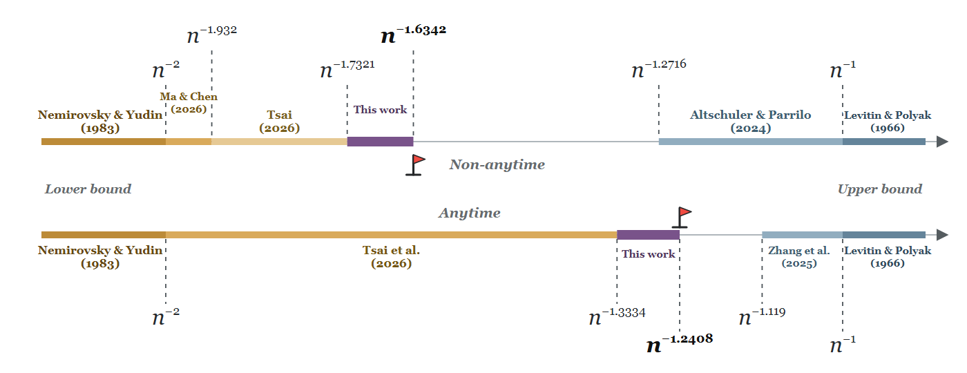
After reviewing additional related work in Section 1.2, we give an overview of our techniques in Section 2. At a high level, both proofs use the hard-function family introduced in ([2], Theorem 4.1). After this construction, Ma and Chen summarize the selected long-step excesses by a single quantity ([2], Section 5.4). Tsai rewrites this quantity in terms of the harmonic mean of these excesses ([14], Lemma 7). In contrast, our main technical contribution is to retain every factor coupling consecutive selected long steps and estimate these factors term by term. For the anytime case, we adapt the finite-to-anytime transfer from ([3], Theorem 4.1) and apply the same estimate at horizons where the last stepsize is the largest seen so far. This yields the improved anytime lower bound.

The remainder of the paper is organized as follows. Section 3 provides the full details of the non-anytime proof outlined in Section 2. Section 4 extends the analysis to the anytime setting. Appendix A recalls the hard-function construction, Appendix B details how the scalar parameters are chosen, and Appendix C contains the proofs deferred from Section 4.

1.2 Related Work

Accelerating GD.

Classical acceleration methods modify GD by incorporating information from previous iterations, as in Polyak's heavy-ball method [9] and Nesterov's accelerated method [10]. A complementary line of work uses the performance-estimation problem (PEP), which provides a systematic numerical framework for worst-case analysis [15]. Interpolation conditions yield exact PEP formulations for fixed-step first-order methods [16]. In the stepsize-only setting, PEP has also been used to search numerically for horizon-dependent GD schedules, providing finite-horizon evidence of acceleration [17, 18]. Within the classical $O(n^{-1})$ regime, improved constants were obtained using predetermined schedules with stepsizes increasing toward $2/L$ [19] and, separately, periodic schedules with occasional long steps analyzed through multi-step certificates [11]. For strongly convex quadratic objectives, stepsize-only acceleration was known much earlier through Chebyshev stepsizes [20]. Fractal orderings were later introduced to control their unstable intermediate iterates [21].

Silver and recursive stepsize schedules.

Let $\rho=1+\sqrt{2}$. At horizons $n=2^k-1$, the recursively defined silver schedule attains the rate $O(n^{-\log_2\rho})$, where $\log_2\rho\approx1.2716$ [4]. A related right-heavy schedule attains the silver exponent for the objective gap, while its reversal attains the same exponent for the squared gradient norm [12]. A subsequent composition framework and an independent concatenation construction extend this rate to every prescribed finite horizon [5, 22]. Note that these guarantees hold at selected horizons (non-anytime case). The question of whether an infinite schedule can accelerate GD at every stopping time was posed in [23] and answered affirmatively in [13], which gives an anytime $O(n^{-1.119})$ rate. The silver-step constructions also extend to projected and proximal gradient methods [24], and to smooth strongly convex objectives with accelerated linear rates [25].

Lower bounds for GD.

The classical $\Omega(n^{-2})$ first-order oracle lower bound for smooth convex optimization goes back to Nemirovsky and Yudin [1], while Nesterov's accelerated method attains the matching $O(n^{-2})$ rate [10]. A standard quadratic-chain proof appears in ([8], Section 2.1.2, Theorem 2.1.7), and we recall its geometric mechanism in Fact 13. Stronger conclusions were previously known under additional structural restrictions. Time-invariant oblivious first-order methods cannot attain $O(n^{-\alpha})$ rates for any $\alpha>1$ ([26], Corollary 1). Within the recursively generated class of basic $f$-composable GD schedules, the best objective-gap rate is $\Theta(n^{-\log_2(1+\sqrt{2})})$ ([5], Theorem 5).

For arbitrary predetermined schedules, an $\Omega(n^{-1.932})$ lower bound was proved using a hard function adapted to the schedule's long steps [2]. The same construction was then used to sharpen the non-anytime bound to $\Omega(n^{-\sqrt{3}})$ [14]. For the anytime case, it was proved in [3] that no positive predetermined infinite schedule satisfies $R_n(H_n)=o(n^{-4/3})$.

2. Technique overview

Section Summary: This section outlines the main steps in proving a polynomial lower bound on the quantity Rn for gradient descent with arbitrary positive step sizes. It first normalizes the problem and selects the largest long steps to derive a product lower bound via Lemma 3, which is then reduced to a sequence inequality (Lemma 4) that couples consecutive terms through the function K while enforcing tail conditions on rearranged weights. The remaining variables are eliminated by passing to a supremum function Γλ whose smoothness, convexity, and monotonicity properties allow the product to be controlled term by term and yield the final rate.

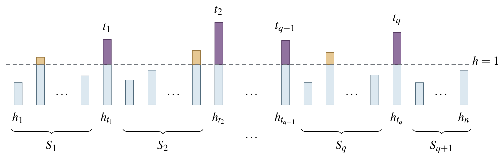
In this section, we provide a high-level overview of techniques behind the proof of Theorem 1. Replacing $f$ by $f/L$ and each $h_k$ by $Lh_k$ leaves the GD iterates and $R_n$ unchanged, so we assume $L=1$ throughout. Following [2], we call a step $h_k$ long if $h_k>1$ and short if $h_k\leq 1$. Let

$ r:=#{k:h_k>1} $

be the number of long steps. For an integer $1\le q\le r$, select $q$ long steps

$ 0<t_1<\cdots<t_q\le n, \qquad h_{t_i}>1, $

where $t_0=0$ and $t_{q+1}=n+1$. Define $S_i$ to be the stepsize accumulation between the selected long steps, that is,

$ S_i:=h_{t_{i-1}+1:t_i-1}, \qquad 1\le i\le q+1, $

where $h_{a:b}:=\sum_{k=a}^b h_k$, with an empty sum equal to zero. An illustration of these concepts is provided in Figure 2.

########## {caption="Lemma 3"}

For every such selection,

$ R_n(H)\ge \frac{1}{S_q+h_{t_q}+2S_{q+1}+1} \prod_{i=1}^{q-1} \frac{S_{i+1}+h_{t_{i+1}}} {S_i+h_{t_i}+S_{i+1}+h_{t_{i+1}}} \prod_{i=1}^{q}\frac{h_{t_i}-1}{S_i+1}.\tag{1} $

This is the lower bound in ([2], Theorem 4.1); see also ([14], Lemma 6). The lemma reduces the original problem to establishing a lower bound for the right-hand side of Equation 1, which involves only the sequence $H$. The lemma extends the classical Huber bound: When no long step is selected ($q=0$), it recovers exactly

$ R_n(H)\ge \frac{1}{1+2\sum_{k=1}^n h_k}.\tag{2} $

We briefly recall the proof of Equation 2 in Fact 12. A nonempty selection $q>0$ allows Equation 1 to adapt flexibly to the long steps, limiting the acceleration they might otherwise provide in Equation 2. The lemma is proved using a hard function tailored to the schedule $H$ and the selected long steps. Appendix A gives an intuitive explanation of the construction.

Based on Lemma 3, Ma and Chen bound the resulting product using a single quantity that summarizes the selected long-step excesses ([2], Section 5.4). Tsai derives a related bound in terms of the harmonic mean of these excesses ([14], Lemma 7) and then uses a counting function ([14], Lemma 8). We instead retain each factor coupling two consecutive selected long steps and estimate these factors term by term.

Reduction to a sequence inequality.

For $w, z, x, y>0$, define

$ K_{w, z}(x, y):= \frac{\sqrt{xy}, (w+z+x+y)} {\sqrt{wz(w+x)(z+y)}}.\tag{3} $

Given any sequence $\omega_1, \ldots, \omega_q$, write $\omega_1^\downarrow\ge\cdots\ge\omega_q^\downarrow$ for its decreasing rearrangement. Then the problem of proving an $\Omega(n^{-(1+\alpha)})$ lower bound for Equation 1 can be reduced to the following sequence inequality.

########## {caption="Lemma 4"}

Fix $\alpha>0$. Suppose there is a constant $C_\alpha<\infty$, depending only on $\alpha$, with the following property: For every integer $q\geq 2$ and any positive sequences $x_1, \ldots, x_q$ and $\omega_1, \ldots, \omega_q$ such that

$ \sum_{i=1}^q x_i<q, \qquad \sum_{s=p+1}^q\omega_s^\downarrow \ge q\left[\left(\frac qp\right)^\alpha-1\right] \quad (\forall 1\le p<q),\tag{4} $

we have

$ E_{\mathrm{end}} \prod_{i=1}^{q-1} K_{\omega_i, \omega_{i+1}}(x_i, x_{i+1}) \le C_\alpha,\tag{5} $

where

$ E_{\mathrm{end}}:= \sqrt{x_1x_q} \sqrt{\frac{1+x_1/\omega_1}{1+x_q/\omega_q}} \left[1+\frac{x_q+2\left(q-\sum_{i=1}^q x_i\right)}{\omega_q} \right].\tag{6} $

Then, $R_n(H)\ge c_\alpha(n+1)^{-(1+\alpha)}$ for every $n$ and $H$.

The reduction makes two choices that are not apparent from Equation 1. Given a cutoff $q$, it selects the $q$ largest excesses, while the cutoff itself is chosen from the schedule $H$ according to 15. The right-hand side of Equation 1 is then normalized so that the variables $x_i$ have total mass below $q$, and the decreasing rearrangement of the weights $\omega_i$ satisfies the tail inequalities in Equation 4. The proof is provided in Section 3.1.

Eliminating the variables xi.

To make Equation 5 tractable, we first eliminate the variables $x_i$. For a parameter $\lambda>0$ to be chosen later, define

$ \Gamma_\lambda(w, z):= \sup_{x, y>0} \left{ \log K_{w, z}(x, y)-\lambda(x+y) \right}.\tag{7} $

By definition,

$ \log K_{w, z}(x, y) \le \lambda(x+y)+\Gamma_\lambda(w, z).\tag{8} $

Applying this inequality to every adjacent factor and using $\sum_i x_i<q$ gives the next reduction.

########## {caption="Lemma 5"}

Fix $\alpha, \lambda>0$. There is a constant $C_{\alpha, \lambda}<\infty$ such that, for every integer $q\ge2$, every pair of positive sequences $(x_i){i=1}^q$ and $(\omega_i){i=1}^q$ satisfying Equation 4 obeys

$ E_{\mathrm{end}} \prod_{i=1}^{q-1}K_{\omega_i, \omega_{i+1}}(x_i, x_{i+1}) \le C_{\alpha, \lambda} \exp!\left{ 2\lambda q+ \sum_{i=1}^{q-1}\Gamma_\lambda(\omega_i, \omega_{i+1}) \right}.\tag{9} $

We are left with a sum of consecutive $\Gamma_\lambda$ terms. To proceed, we record some basic properties of $\Gamma_\lambda$.

########## {caption="Lemma 6: Properties of $\Gamma_\lambda$ "}

For every $\lambda>0$, $\Gamma_\lambda$ has the following properties.

1. Smoothness. For every $w, z>0$, the supremum in Equation 7 is attained at a unique point of $(0, \infty)^2$. Denote this point by $(x_\lambda(w, z), y_\lambda(w, z))$. The optimizer map and $\Gamma_\lambda$ are $C^\infty$ on $(0, \infty)^2$.
2. Symmetry. $\Gamma_\lambda(w, z)=\Gamma_\lambda(z, w)$.
3. Joint convexity. The map $(w, z)\mapsto\Gamma_\lambda(w, z)$ is jointly convex on $(0, \infty)^2$.
4. Coordinatewise decrease. The function $\Gamma_\lambda$ is strictly decreasing in each coordinate.
5. Strict submodularity.

$ \partial_{wz}^2\Gamma_\lambda(w, z)<0.\tag{10} $

Controlling the summation of consecutive pairs.

The remaining sum is bounded in four steps. First, the summation of consecutive pairs can be split into two matchings, and maximizing over matchings leads to a symmetric function. Second, the symmetry, joint convexity, and coordinatewise decrease together allow majorization, replacing the unknown weights $\omega_i^\downarrow$ by the explicit comparison sequence in Equation 23. Third, strict submodularity identifies the maximizing matching of these explicit comparison weights. Finally, the resulting finite sum is compared with a one-dimensional integral. The full argument is given in Section 3.4.

########## {caption="Lemma 7"}

Fix $\alpha, \lambda>0$. There is a constant $C_{\alpha, \lambda}<\infty$ such that, for every integer $q\ge2$ and every positive sequence $\omega_1, \ldots, \omega_q$ satisfying the tail condition in Equation 4,

$ \sum_{i=1}^{q-1}\Gamma_\lambda(\omega_i, \omega_{i+1}) \le 2q\int_0^{1/2} \Gamma_\lambda\bigl(W_\alpha(t), W_\alpha(1-t)\bigr), dt +C_{\alpha, \lambda},\tag{11} $

where $W_\alpha(t):=\alpha t^{-1-\alpha}$ for $0<t\le1$.

Completing the proof of Theorem 1.1.

Define

$ J(\alpha, \lambda) :=2\lambda+ 2\int_0^{1/2} \Gamma_\lambda\bigl(W_\alpha(t), W_\alpha(1-t)\bigr), dt.\tag{12} $

Then Lemma 5 and Lemma 7 give

$ E_{\mathrm{end}} \prod_{i=1}^{q-1}K_{\omega_i, \omega_{i+1}}(x_i, x_{i+1}) \le C_{\alpha, \lambda}e^{qJ(\alpha, \lambda)}.\tag{13} $

Thus $J(\alpha, \lambda)\le0$ makes Equation 5 uniform in $q$, and Lemma 4 yields

$ R_n(H)\ge c_{\alpha, \lambda}(n+1)^{-(1+\alpha)}.\tag{14} $

For $\alpha=0.6342$ and $\lambda=0.4506$, numerical integration gives $J(0.6342, 0.4506)<-0.00005<0$. Therefore $R_n(H)=\Omega(n^{-1.6342})$, proving Theorem 1. Appendix B studies the dependence of $J$ on $(\alpha, \lambda)$ and explains how the pair $(0.6342, 0.4506)$ was obtained numerically.

3. Proof of the Non-Anytime Lower Bound

Section Summary: This section delivers the complete technical proofs of Lemmas 4–7 establishing a non-asymptotic lower bound on the remainder term R_n(H) for any schedule of n steps. It first reduces the problem to a finite-dimensional sequence inequality by splitting each step size into a bounded base component and ordered excess components, then selects a distinguished index q that controls the accumulation D_q and applies a specialized comparison lemma to obtain the explicit power-law bound c_α(n+1)^(-(1+α)). Subsequent subsections remove auxiliary variables through logarithmic estimates and exponential tail bounds, verify smoothness and convexity properties of an auxiliary function Γ_λ, and thereby confirm that the constants remain uniform.

This section provides the full proofs of Lemma 4, Lemma 5, Lemma 6, and Lemma 7.

3.1 Reduction to a sequence inequality

Proof of Lemma 4: Suppose that Equation 4 implies Equation 5, with a constant $C_\alpha$ uniform over all $q\ge 2$. Fix $n\ge 1$ and a schedule $H=(h_1, \ldots, h_n)$. Recall that $r$ is the number of long steps. If $r=0$, the Huber bound Equation 2 yields

$ R_n(H)\ge(2n+1)^{-1}\ge(2(n+1))^{-1}. $

Therefore, from now on we consider $r\geq 1$.

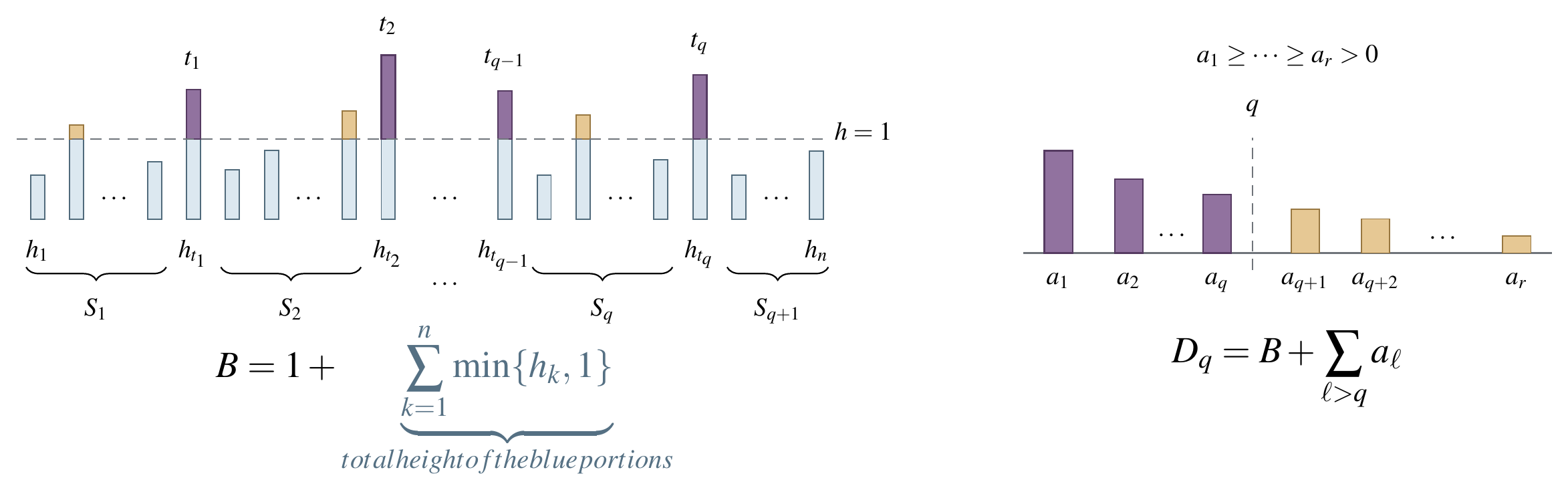
We decompose each stepsize $h_k$ into two components: a base $\min{h_k, 1}$ and an excess $\max{h_k - 1, 0}$. Let $a_1 \ge \cdots \ge a_r > 0$ denote the positive excesses in decreasing order. We define the base accumulation as $B:=1+\sum_{k=1}^n\min{h_k, 1}$. By definition, $B\leq n+1$. Moreover, let $D_s$ denote the total stepsize accumulation excluding the excesses from the $s$ longest steps:

$ D_s:=B+\sum_{\ell=s+1}^r a_\ell, \qquad 1\le s\le r, $

with $D_r=B$. See Figure 3 for an illustration of these definitions.

Choose

$ q\in\operatorname*{arg, min}_{1\le s\le r}D_s s^\alpha.\tag{15} $

This specific choice ensures that $D_q$ has a universal upper bound

$ D_q\leq D_q q^\alpha \le D_r r^\alpha \leq (n+1)^{\alpha+1}\tag{16} $

as $D_r=B\leq n+1$ and $r+1\leq n+1$.

We first treat the special case $q=1$ to illustrate the power of Lemma 3. Then we show that Lemma 3 combined with Equation 5 is sufficient to prove the general case $q\geq 2$.

Case 1: $q=1$.

If $a_1\le D_1$, since $D_1+a_1=1+\sum_{k=1}^n h_k$, the Huber bound Equation 2 gives

$ R_n(H)\ge \frac1{2(D_1+a_1)-1} \ge \frac1{4D_1}. $

If $a_1>D_1$, select $t$ such that $h_t-1=a_1$ and apply Lemma 3. In this case $D_1=(S_1+1)+(S_2+1)$, while

$ (S_1+1)+a_1+2(S_2+1)-1<a_1+2D_1<3a_1. $

Consequently,

$ R_n(H) \ge\frac{a_1}{(S_1+1)(S_1+a_1+2S_2+2)}

\frac1{3(S_1+1)} \ge\frac1{3D_1} \frac1{4D_1}. $

Thus $R_n(H)\ge1/(4D_1)$ in both subcases. Applying Equation 16 yields

$ R_n(H)\ge\frac1{4(n+1)^{\alpha+1}}. $

Case 2: $q\ge 2$.

Let $t_1<\cdots<t_q$ be the indices of the $q$ largest positive excesses $h_k-1$. With this selection, let $S_1, \ldots, S_{q+1}$ be defined as in Lemma 3. Note that

$ \sum_{i=1}^{q+1}(S_i+1) =q+1+\sum_{k\notin{t_1, \ldots, t_q}}h_k =D_q. $

We use $D_q/q$ as the normalization scale for $S_i+1$ and $h_{t_i}-1$, and define

$ x_i:=\frac{q(S_i+1)}{D_q}, \qquad \omega_i:=\frac{q(h_{t_i}-1)}{D_q}, \qquad 1\le i\le q. $

By Lemma 3, $R_n(H)\ge G$, where $G$ denotes the right-hand side of Equation 1 for the indices selected above. Substituting the definitions of $x_i$ and $\omega_i$ gives

$ G^{-1} =\frac{D_q}{q}\sqrt{x_1x_q} \sqrt{\frac{1+x_1/\omega_1}{1+x_q/\omega_q}} \left[1+\frac{x_q+2(q-\sum_{i=1}^q x_i)-q/D_q}{\omega_q} \right] \prod_{i=1}^{q-1} K_{\omega_i, \omega_{i+1}}(x_i, x_{i+1}). $

Replacing $-q/D_q$ by $0$ increases the quantity in the bracket and yields

$ G^{-1}\le \frac{D_q}{q}E_{\mathrm{end}}\prod_{i=1}^{q-1}K_{\omega_i, \omega_{i+1}}(x_i, x_{i+1}).\tag{17} $

The sequences $(x_i){i=1}^q$ and $(\omega_i){i=1}^q$ satisfy Equation 4. Specifically, as $x_i$ are normalized,

$ \sum_{i=1}^q x_i =\frac q{D_q}\sum_{i=1}^q(S_i+1) =q-\frac{q(S_{q+1}+1)}{D_q} <q. $

Moreover, noting that $\omega_s^\downarrow=qa_s/D_q$ for $1\le s\le q$, the minimizing property Equation 15 implies

$ 1+\frac1q\sum_{s=p+1}^q\omega_s^\downarrow =1+\frac{\sum_{s=p+1}^q a_s}{D_q} =\frac{D_p}{D_q} \ge \left(\frac qp\right)^\alpha $

for every $1\le p<q$. Hence, Equation 5 holds, and by Equation 16,

$ R_n(H)\ge G\ge\frac{q}{C_\alpha D_q}\geq\frac{1}{C_\alpha (n+1)^{\alpha+1}}. $

Finally, combining all cases gives

$ R_n(H)\ge c_\alpha(n+1)^{-(1+\alpha)}, \qquad c_\alpha:=\min{C_\alpha^{-1}, 1/4}. $

3.2 Eliminating the variables xi

Proof of Lemma 5: Set

$ \Delta:=q-\sum_{i=1}^q x_i>0. $

Applying Equation 8 to $K_{\omega_i, \omega_{i+1}}(x_i, x_{i+1})$ for $1\le i<q$ and summing gives

$ \log\prod_{i=1}^{q-1} K_{\omega_i, \omega_{i+1}}(x_i, x_{i+1}) \le \lambda\sum_{i=1}^{q-1}(x_i+x_{i+1}) +\sum_{i=1}^{q-1}\Gamma_\lambda(\omega_i, \omega_{i+1}). $

Since

$ \sum_{i=1}^{q-1}(x_i+x_{i+1}) =2\sum_{i=1}^q x_i-x_1-x_q =2q-(2\Delta+x_1+x_q), $

we obtain

$ \begin{aligned} E_{\mathrm{end}} \prod_{i=1}^{q-1}K_{\omega_i, \omega_{i+1}}(x_i, x_{i+1}) &\le \exp!\left{ 2\lambda q+\sum_{i=1}^{q-1} \Gamma_\lambda(\omega_i, \omega_{i+1}) \right} E_{\mathrm{end}} e^{-\lambda(2\Delta+x_1+x_q)}. \end{aligned} $

It remains to bound $E_{\mathrm{end}}e^{-\lambda(2\Delta+x_1+x_q)}$ independently of $q$, $(x_i){i=1}^q$, and $(\omega_i){i=1}^q$.

Taking $p=q-1$ in Equation 4 yields

$ \min_{1\le i\le q}\omega_i =\omega_q^\downarrow \ge q\left[\left(\frac q{q-1}\right)^\alpha-1\right] \ge\alpha q\log\frac q{q-1} \ge\alpha.\tag{18} $

The last two inequalities use $e^u-1\ge u$ and $\log(1+t)\ge t/(1+t)$. In particular, $\omega_1, \omega_q\ge\alpha$. Using this in Equation 6 and writing $T:=x_1+x_q+\Delta$, we obtain

$ E_{\mathrm{end}}e^{-\lambda(2\Delta+x_1+x_q)} \le C_\alpha(1+T)^{5/2}e^{-\lambda T} \le C_\alpha\sup_{t\ge0}(1+t)^{5/2}e^{-\lambda t} =:C_{\alpha, \lambda}<\infty. $

Substitution into the preceding display proves Equation 9.

3.3 Properties of Gamma lambda

Proof of Lemma 6: For $w, z, x, y>0$, set

$ F_{w, z}(x, y):=\log K_{w, z}(x, y)-\lambda(x+y). $

(1) Smoothness.

For fixed $w, z>0$, the function $F_{w, z}(x, y)$ tends to $-\infty$ as $x\downarrow0$, $y\downarrow0$, or $x+y\to\infty$. It therefore attains its maximum at an interior point. Write $A:=w+x$, $B:=z+y$, and $\Sigma:=A+B$. For every nonzero direction $(a, b)$,

$ D^2_{x, y}F_{w, z}(x, y)[(a, b), (a, b)] =-\frac{a^2}{2x^2}-\frac{b^2}{2y^2} -\frac{(a+b)^2}{\Sigma^2} +\frac{a^2}{2A^2}+\frac{b^2}{2B^2}<0. $

Thus the maximizer is unique.

Fix $(w_0, z_0)$ and let $(x_0, y_0)$ be its maximizer. The Jacobian in $(x, y)$ of the first-order condition $\nabla_{x, y}F_{w, z}(x, y)=0$ is the invertible Hessian above. The implicit function theorem gives a neighborhood of $(w_0, z_0)$ on which the critical point is a $C^\infty$ function of $(w, z)$. Since $(w_0, z_0)$ was arbitrary, the optimizer map is $C^\infty$ on $(0, \infty)^2$. Substituting it into $F_{w, z}$ shows that $\Gamma_\lambda$ is also $C^\infty$.

(2) Symmetry.

The definition 7 is invariant under $(w, x)\leftrightarrow(z, y)$.

(3) Joint convexity.

For fixed $x, y$, put $A:=w+x$ and $B:=z+y$. The Hessian in $(w, z)$ has quadratic form

$ D^2_{w, z}F_{w, z}(x, y)[(a, b), (a, b)]=\frac{a^2}{2w^2}+\frac{a^2}{2A^2} +\frac{b^2}{2z^2}+\frac{b^2}{2B^2} -\frac{(a+b)^2}{(A+B)^2}\ge0. $

Indeed, the first four terms dominate $a^2/A^2+b^2/B^2$, which is at least $(a+b)^2/(A+B)^2$ by Cauchy–Schwarz. Taking the supremum in Equation 7 preserves convexity.

(4) Coordinatewise decrease.

Write $x_*:=x_\lambda(w, z)$ and $y_*:=y_\lambda(w, z)$, and set $A:=w+x_*$, $B:=z+y_*$, and $\Sigma:=A+B$. The chain rule and the first-order conditions give

$ \begin{aligned}\partial_w\Gamma_\lambda &=\partial_wF_{w, z} +\partial_xF_{w, z}, \partial_wx_* +\partial_yF_{w, z}, \partial_wy_*\&=\partial_wF_{w, z} =\frac1\Sigma-\frac1{2w}-\frac1{2A}.\end{aligned}\tag{19} $

Equivalently,

$ -\partial_w\Gamma_\lambda =\frac{x_*}{2wA}+\frac{B}{A\Sigma}>0, $

and the same argument applies to the $z$ coordinate.

(5) Strict submodularity.

With the notation above, the first-order conditions imply

$ \lambda-\frac1\Sigma =\frac{w}{2x_*A} =\frac{z}{2y_*B}. $

Consequently, define the parameter

$ \tau_*:=\frac{x_*A}{w}=\frac{y_*B}{z}>0. $

For $u, \tau>0$, set

$ f_u(\tau):=\frac{u+\sqrt{u^2+4u\tau}}2.\tag{20} $

Then $x_*=-w+f_w(\tau_*)$, $y_*=-z+f_z(\tau_*)$, $A=f_w(\tau_*)$, $B=f_z(\tau_*)$, and

$ g(\tau_*;w, z)=0, \qquad g(\tau;w, z):= \frac1{2\tau}+\frac1{f_w(\tau)+f_z(\tau)}-\lambda.\tag{21} $

The explicit formula for $f_u$ shows that it increases in both arguments. Hence $\partial_\tau g<0$ and $\partial_zg<0$, and implicit differentiation gives $\partial_z\tau_*=-(\partial_zg)/(\partial_\tau g)<0$. Moreover,

$ \Sigma=\left(\lambda-\frac1{2\tau_*}\right)^{-1}, \qquad A=f_w(\tau_*). $

Since $d\Sigma/d\tau=-\Sigma^2/(2\tau^2)<0$, we have $\partial_z\Sigma>0$ and $\partial_zA=f_w'(\tau_*)\partial_z\tau_*<0$. Differentiating Equation 19 yields

$ \partial_{wz}^2\Gamma_\lambda =-\frac{\partial_z\Sigma}{\Sigma^2} +\frac{\partial_zA}{2A^2}<0, $

which proves Equation 10.

3.4 Upper bounding $\sum_{i=1}^{q-1}\Gamma_\lambda(\omega_i, \omega_{i+1})$

In this section, we prove Lemma 7.

Step 1. Symmetrization.

For a positive vector $v=(v_1, \ldots, v_N)\in\mathbb{R}^N$ and $0\le k\le\lfloor N/2\rfloor$, let $\mathcal M_k(N)$ be the set of all collections of $k$ disjoint unordered pairs from ${1, \ldots, N}$. Define the largest sum over all $k$-edge matchings on the coordinates of $v$ to be

$ \Phi_{k, \lambda}(v_1, \ldots, v_N) :=\max_{M\in\mathcal M_k(N)} \sum_{{a, b}\in M}\Gamma_\lambda(v_a, v_b), \qquad \Phi_{0, \lambda}:=0. $

Let $N=q-1$ and

$ k_q:=\left\lfloor\frac{q-1}{2}\right\rfloor. $

We are going to show that

$ \sum_{i=1}^{q-1}\Gamma_\lambda(\omega_i, \omega_{i+1}) \le 2\Phi_{k_q, \lambda} (\omega_q^\downarrow, \ldots, \omega_2^\downarrow) +C_{\alpha, \lambda}.\tag{22} $

We first split the consecutive pairs into an odd matching and an even matching, according to whether $i$ is odd or even. An illustration is given in Figure 4.

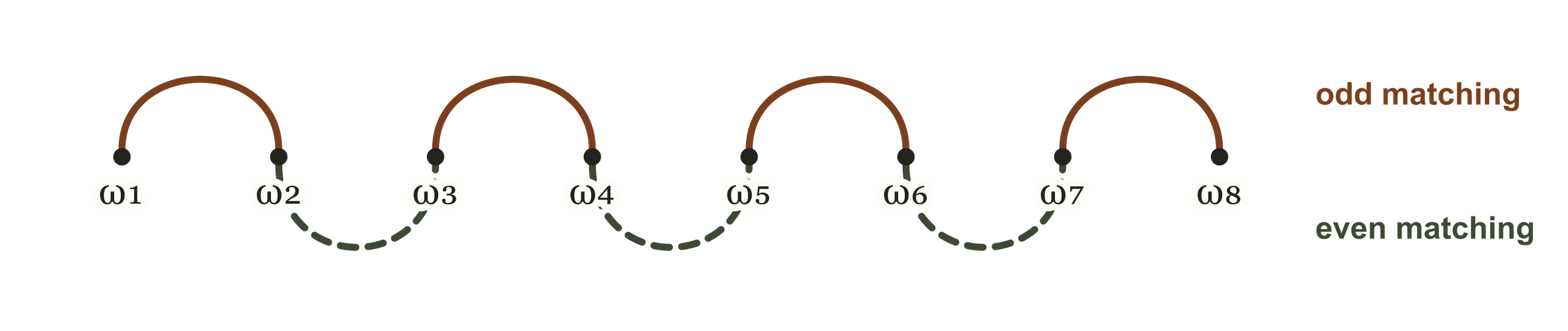
Choose $i_*$ such that $\omega_{i_*}=\omega_1^\downarrow$. If $q$ is odd, both matchings have $k_q$ pairs and leave one index unused. If $i_*$ is matched, replace it by the unused index. The unused coordinate has no larger value, so the coordinatewise decrease in Lemma 6 shows that the matching sum cannot decrease. If $q$ is even, the same replacement applies to the even matching with $k_q$ pairs. The odd matching has $k_q+1$ pairs. Delete the pair containing $i_*$. The remaining matching has $k_q$ pairs drawn from $(\omega_q^\downarrow, \ldots, \omega_2^\downarrow)$, and is therefore bounded by $\Phi_{k_q, \lambda}(\omega_q^\downarrow, \ldots, \omega_2^\downarrow)$. By Equation 18, every $\omega_i\ge\alpha$, and coordinatewise decrease gives $\Gamma_\lambda(\omega_i, \omega_j)\le\Gamma_\lambda(\alpha, \alpha)$. In particular, the contribution of the deleted pair is bounded by $\max{0, \Gamma_\lambda(\alpha, \alpha)}$. This proves Equation 22.

Step 2. Majorization.

For a fixed matching, the sum of its $\Gamma_\lambda$ terms is convex and coordinatewise decreasing. Taking the maximum over all matchings preserves both properties, and permuting the coordinates only permutes the matchings. Thus $\Phi_{k, \lambda}$ is symmetric, convex, and coordinatewise decreasing. For a symmetric, convex, and coordinatewise decreasing function, we have the following majorization principle:

########## {caption="Lemma 8"}

Let $F:(0, \infty)^N\to\mathbb{R}$ be symmetric, convex, and coordinatewise decreasing. Suppose $a_1\le\cdots\le a_N$ and $b_1\le\cdots\le b_N$ satisfy

$ \sum_{i=1}^{\ell}a_i\ge\sum_{i=1}^{\ell}b_i, \qquad 1\le\ell\le N. $

Then $F(a)\le F(b)$.

Here, the partial-sum assumption is precisely $a\prec^{, w}b$, in the notation of weak supermajorization. Since every symmetric convex function is Schur-convex and $F$ is coordinatewise decreasing, the conclusion $F(a)\le F(b)$ follows from the standard characterization of functions preserving weak supermajorization; see ([27], Theorem 3.A.8 and Proposition 3.C.2).

For $2\le s\le q$, define the comparison weights

$ \bar{w}_s^{(q)} :=q^{1+\alpha}\bigl((s-1)^{-\alpha}-s^{-\alpha}\bigr),\tag{23} $

which may also be written as

$ \bar{w}s^{(q)} =q^{1+\alpha}\int{s-1}^{s}\alpha u^{-1-\alpha}, du. $

Since the integrand is decreasing, $\bar{w}_q^{(q)}\le\cdots\le\bar{w}_2^{(q)}$. Moreover, for $1\le p<q$,

$ \sum_{s=p+1}^q\bar{w}_s^{(q)} =q^{1+\alpha}\int_p^q\alpha u^{-1-\alpha}, du =q\left[\left(\frac qp\right)^\alpha-1\right]. $

Setting $p=q-\ell$ in Equation 4 gives, for $1\le\ell\le q-1$,

$ \sum_{i=1}^{\ell}\omega_{q+1-i}^\downarrow \ge\sum_{i=1}^{\ell}\bar{w}_{q+1-i}^{(q)}. $

Applying Lemma 8 to $F=\Phi_{k_q, \lambda}$, $a=(\omega_q^\downarrow, \ldots, \omega_2^\downarrow)$, and $b=(\bar{w}_q^{(q)}, \ldots, \bar{w}_2^{(q)})$ proves

$ \Phi_{k_q, \lambda} (\omega_q^\downarrow, \ldots, \omega_2^\downarrow) \le \Phi_{k_q, \lambda} (\bar{w}_q^{(q)}, \ldots, \bar{w}_2^{(q)}).\tag{24} $

Step 3. Identify the maximizing matching.

Majorization has replaced the unknown weights by the explicit sequence $(\bar{w}_q^{(q)}, \ldots, \bar{w}_2^{(q)})$. It remains to identify the matching that maximizes the resulting sum.

For $0<a\le b\le c\le d$, symmetry and strict submodularity give

$ \begin{aligned} \Gamma_\lambda(a, d)+\Gamma_\lambda(b, c) &\ge\Gamma_\lambda(a, c)+\Gamma_\lambda(b, d), \ \Gamma_\lambda(a, d)+\Gamma_\lambda(b, c) &\ge\Gamma_\lambda(a, b)+\Gamma_\lambda(c, d). \end{aligned} $

Let $0<v_1\le\cdots\le v_N$. Since $\Gamma_\lambda$ decreases in each coordinate, a maximizing matching may be chosen to use the $2k$ smallest coordinates. If $v_1$ is not paired with $v_{2k}$, exchange the partners of their two pairs. The two inequalities above show that the total cannot decrease. Fixing the pair $(v_1, v_{2k})$ and repeating on the remaining coordinates gives

$ \Phi_{k, \lambda}(v_1, \ldots, v_N) =\sum_{j=1}^k\Gamma_\lambda(v_j, v_{2k+1-j}).\tag{25} $

Applied to the comparison weights, this identity gives

$ \Phi_{k_q, \lambda}(\bar{w}q^{(q)}, \ldots, \bar{w}2^{(q)}) =\sum{j=1}^{k_q} \Gamma\lambda (\bar{w}{q+1-j}^{(q)}, \bar{w}{q-2k_q+j}^{(q)}).\tag{26} $

Step 4. Comparison with the integral.

Finally, we estimate $\sum_{j=1}^{k_q}\Gamma_\lambda(\bar{w}{q+1-j}^{(q)}, \bar{w}{q-2k_q+j}^{(q)})$ by comparing it with its corresponding Riemann integral. By the mean value theorem, for every $2\le s\le q$ there is $\theta_s\in(s-1, s)$ such that

$ \bar{w}s^{(q)}=W\alpha(\theta_s/q), \qquad W_\alpha(t):=\alpha t^{-1-\alpha}, \quad 0<t\le1.\tag{27} $

To control the error introduced by replacing these mean-value points with the uniform mesh, define

$ G(t, v):=\Gamma_\lambda(W_\alpha(t), W_\alpha(v)), \qquad 0<t\le1, \quad 0< v\le1. $

The following regularity estimate shows that one argument of $G$ can be extended to $0$.

########## {caption="Lemma 9: Uniform Lipschitz bound"}

For fixed $\alpha, \lambda>0$, the function $G$ has a Lipschitz extension to $[0, 1]\times[1/2, 1]$.

Proof of Lemma 9: Let $D:=(0, 1]\times[1/2, 1]$. For $(t, v)\in D$, write $w:=W_\alpha(t), z:=W_\alpha(v)$, and let $(x_*, y_*)$ be the unique optimizer in the definition of $\Gamma_\lambda(w, z)$. Set $A:=w+x_*, B:=z+y_*, \Sigma:=A+B$ as in the proof of Lemma 6. The first-order conditions give

$ \tau_*:=\frac{x_*A}{w}=\frac{y_B}{z}, \qquad \lambda=\frac{1}{2\tau_}+\frac{1}{\Sigma}. $

We first obtain bounds on the optimizer that are uniform over $D$. Since $v\in[1/2, 1]$,

$ \alpha\le z\le \alpha 2^{1+\alpha}. $

Moreover, as $z+y_*\ge\sqrt{z\tau_*}$,

$ \lambda \le\frac1{2\tau_*}+\frac1{\sqrt{\alpha\tau_*}}. $

The right-hand side tends to $0$ as $\tau_*\to\infty$, so $\tau_*\le C_{\alpha, \lambda}$. In particular, $x_*, y_*\le\tau_*\le C_{\alpha, \lambda}$. The bounds on $z$ and $y_*$ give $B:=z+y_*\le\alpha2^{1+\alpha}+C_{\alpha, \lambda}$, whereas $A:=w+x_*\ge w$ and $\Sigma:=A+B\ge w$.

We next bound the derivatives of $\Gamma_\lambda$. The derivative identity Equation 19 yields

$ -\partial_w\Gamma_\lambda(w, z) =\frac{x_*}{2wA}+\frac{B}{A\Sigma}. $

Since $A\ge w$, $\Sigma\ge A\ge w$, and $x_*, B\le C_{\alpha, \lambda}$, $\left|\partial_w\Gamma_\lambda(w, z)\right|\le C_{\alpha, \lambda}w^{-2}$. Similarly,

$ -\partial_z\Gamma_\lambda(w, z) =\frac{y_*}{2zB}+\frac{A}{B\Sigma}. $

Using $z, B\ge\alpha$, $y_*\le C_{\alpha, \lambda}$, and $A\le\Sigma$, we obtain $\left|\partial_z\Gamma_\lambda(w, z)\right|\le \frac{C_{\alpha, \lambda}}{2\alpha^2}+\frac1\alpha\le C_{\alpha, \lambda}$.

By the chain rule,

$ \partial_tG(t, v) =\partial_w\Gamma_\lambda(w, z), W_\alpha'(t). $

Since $|W_\alpha'(t)|=\alpha(1+\alpha)t^{-2-\alpha}$ and $W_\alpha(t)^{-2}=\alpha^{-2}t^{2+2\alpha}$, we have

$ |\partial_tG(t, v)| \le C_{\alpha, \lambda} |W_\alpha'(t)|W_\alpha(t)^{-2} \le C_{\alpha, \lambda}t^\alpha \le C_{\alpha, \lambda}. $

Likewise,

$ \partial_vG(t, v) =\partial_z\Gamma_\lambda(w, z), W_\alpha'(v). $

Because $v\in[1/2, 1]$, the derivative $W_\alpha'(v)$ is uniformly bounded, and hence

$ |\partial_vG(t, v)|\le C_{\alpha, \lambda}. $

It follows that $G$ is uniformly Lipschitz on $D$.

In particular, for every $v\in[1/2, 1]$, the limit

$ \overline{G}(0, v):=\lim_{t\downarrow0}G(t, v) $

exists. Defining $\overline{G}=G$ on $D$ and using these limits on ${0}\times[1/2, 1]$, the preceding Lipschitz estimate passes to the limit. Hence $\overline{G}$ is a Lipschitz extension of $G$ to $[0, 1]\times[1/2, 1]$.

Using this extension, define

$ I(t):=G(t, 1-t), \qquad 0\le t\le\frac12. $

After increasing the Lipschitz constant if needed, there are finite $L_{\alpha, \lambda}$ and $M_{\alpha, \lambda}$ such that

$ \begin{aligned} |G(t, v)-G(t', v')| &\le L_{\alpha, \lambda}(|t-t'|+|v-v'|), \ |I(t)-I(t')| &\le L_{\alpha, \lambda}|t-t'|, \qquad |I(t)|\le M_{\alpha, \lambda}. \end{aligned} $

Assume first that $q\ge3$, and write

$ r_q:=q-2k_q\in{1, 2}, \qquad u_j:=\frac{r_q+j-1}{q}, \qquad 1\le j\le k_q. $

By symmetry and 26,

$ \Phi_{k_q, \lambda}(\bar{w}q^{(q)}, \ldots, \bar{w}2^{(q)}) =\sum{j=1}^{k_q} G\left(\frac{\theta{r_q+j}}q, \frac{\theta_{q+1-j}}q\right). $

Moreover,

$ \frac{\theta_{r_q+j}}q \in\left(u_j, u_j+\frac1q\right), \qquad \frac{\theta_{q+1-j}}q \in\left(1-u_j+\frac{r_q-1}{q}, 1-u_j+\frac{r_q}{q}\right). $

The total displacement from $(u_j, 1-u_j)$ is less than $(1+r_q)/q\le3/q$. Since $k_q\le q/2$,

$ \left| \Phi_{k_q, \lambda}(\bar{w}q^{(q)}, \ldots, \bar{w}2^{(q)}) -\sum{j=1}^{k_q}I(u_j) \right| \le\frac32L{\alpha, \lambda}. $

The intervals $[u_j-1/q, u_j]$ are consecutive, and at most $1/q$ of $[0, 1/2]$ is omitted: For odd $q$, they fill $[0, 1/2-1/(2q)]$; for even $q$, they fill $[1/q, 1/2]$. On each covered interval, replacing $I(t)$ by its value at the right endpoint costs at most $L_{\alpha, \lambda}/(2q)$. Hence

$ \left| \sum_{j=1}^{k_q}I(u_j) -q\int_0^{1/2}I(t), dt \right| \le\frac14L_{\alpha, \lambda}+M_{\alpha, \lambda}. $

Combining the two comparisons gives

$ \begin{aligned} \Phi_{k_q, \lambda}(\bar{w}q^{(q)}, \ldots, \bar{w}2^{(q)}) &=\sum{j=1}^{k_q}I(u_j)+O{\alpha, \lambda}(1)\ &=q\int_0^{1/2} \Gamma_\lambda(W_\alpha(t), W_\alpha(1-t)), dt +O_{\alpha, \lambda}(1). \end{aligned} $

When $q=2$, $k_q=0$, and the same estimate holds after enlarging the constant. Combining this estimate with Equation 22 and 24 proves Equation 11.

4. Anytime Lower Bound

Section Summary: This section extends the paper's core lower bound technique to the anytime setting, where a single infinite schedule must be chosen in advance and its consistent prefixes applied at every horizon. The added consistency requirement produces a sharper impossibility result: no schedule can drive the regret below Ω(n^{-1.2408}). The argument proceeds by reducing the problem to a truncated sequence inequality, deriving a suitable product bound that absorbs the truncation error, and verifying numerically that a key exponent J(α, λ) remains negative for α ≈ 0.6342, which directly yields the stated rate.

In this section, we further extend the improved lower bound to the anytime case, for which an infinite schedule $h=(h_k)_{k\geq 1}$ is fixed in advance, and its prefix $H_n=(h_1, \ldots, h_n)$ is used at horizon $n$. Compared with the non-anytime case, the schedules used at different horizons must be consistent. This leads to a sharper $\Omega(n^{-1.2408})$ lower bound. As a high-level conclusion of the proof, we combine the term-by-term estimate from the preceding sections with the anytime transfer argument of [3].

We first reduce the anytime problem to a truncated sequence inequality, similar to Lemma 4.

########## {caption="Lemma 10"}

Fix $\alpha>0$. Suppose that there are constants $\eta_\alpha\in(0, 1)$ and $C_\alpha<\infty$, depending only on $\alpha$, with the following property: For every integer $q\geq 2$, every integer $1\leq \ell\leq \eta_\alpha q$, and all positive sequences $(x_i){i=1}^q$ and $(\omega_i){i=1}^q$ such that

$ \sum_{i=1}^q x_i<q, \qquad \sum_{s=k+1}^q\omega_s^\downarrow \geq q\left[\left(\frac qk\right)^\alpha-1\right] \quad (\forall \ell\leq k<q),\tag{28} $

we have

$ E_{\mathrm{end}} \prod_{i=1}^{q-1} K_{\omega_i, \omega_{i+1}}(x_i, x_{i+1}) \leq C_\alpha,\tag{29} $

where $E_{\mathrm{end}}$ and $K_{\omega_i, \omega_{i+1}}(x_i, x_{i+1})$ are defined as in Lemma 4.

Then every positive infinite schedule satisfies $\limsup_{n\to\infty}n^{\frac{2(1+\alpha)}{2+\alpha}}R_n(H_n)>0$.

When $\ell=1$, Equation 28 coincides with Equation 4. For $\ell>1$, the constraints indexed by $1\leq k<\ell$ are removed, so the $\ell$ largest $\omega_i$ are unconstrained. Thus Equation 28 admits a larger class of sequences $(x_i){i=1}^q$ and $(\omega_i){i=1}^q$ than Equation 4.

To proceed, we adapt the estimation technique in the proof of Lemma 7 to the truncated tail condition Equation 28. The resulting product bound has exponent $qJ(\alpha, \lambda)+O_{\alpha, \lambda}(\ell+1)$, rather than $qJ(\alpha, \lambda)$ as in Equation 13.

########## {caption="Lemma 11"}

Fix $\alpha, \lambda>0$. There are constants $A_{\alpha, \lambda}>0$ and $B_{\alpha, \lambda}\geq0$, depending only on $\alpha$ and $\lambda$, such that, for every $q\geq2$, every $1\leq\ell<q$, and all positive sequences $(x_i){i=1}^q$ and $(\omega_i){i=1}^q$ satisfying Equation 28,

$ E_{\mathrm{end}} \prod_{i=1}^{q-1} K_{\omega_i, \omega_{i+1}}(x_i, x_{i+1}) \leq A_{\alpha, \lambda} \exp!\left{ qJ(\alpha, \lambda)+B_{\alpha, \lambda}(\ell+1) \right}.\tag{30} $

Appendix C contains the proof of the lemmas above.

Completing the proof of Theorem 1.2.

Suppose that $J(\alpha, \lambda)<0$, and choose $\eta_\alpha\in(0, 1)$ so that $B_{\alpha, \lambda}\eta_\alpha\leq-J(\alpha, \lambda)/2$. For every $q\geq2$, every integer $1\leq\ell\leq\eta_\alpha q$, and all positive sequences $(x_i){i=1}^q$ and $(\omega_i){i=1}^q$ satisfying Equation 28, Lemma 11 gives

$ E_{\mathrm{end}} \prod_{i=1}^{q-1}K_{\omega_i, \omega_{i+1}}(x_i, x_{i+1}) \leq A_{\alpha, \lambda} e^{qJ(\alpha, \lambda)+B_{\alpha, \lambda}(\ell+1)} \leq A_{\alpha, \lambda}e^{B_{\alpha, \lambda}} e^{qJ(\alpha, \lambda)/2} \leq C_{\alpha, \lambda}.\tag{31} $

Thus Equation 29 is uniform in $q$ and $\ell$, and Lemma 10 yields, for every positive infinite schedule,

$ \limsup_{n\to\infty} n^{\frac{2(1+\alpha)}{2+\alpha}}R_n(H_n)>0.\tag{32} $

It remains only to find a pair $(\alpha, \lambda)$ for which $J(\alpha, \lambda)<0$. For $\alpha=0.6342$ and $\lambda=0.4506$, numerical integration gives $J(0.6342, 0.4506)<-0.00005<0$. Since $2(1+0.6342)/(2+0.6342)=1.240756\ldots<1.2408$, no positive infinite schedule satisfies $R_n(H_n)=o(n^{-1.2408})$. Appendix B explains the optimization over $(\alpha, \lambda)$ and the numerical verification.

5. Concluding Remarks

Section Summary: This paper tightens the theoretical lower bounds on how fast gradient descent with fixed step sizes can converge, both in standard settings and in anytime versions that must work across varying horizons. It leaves open the larger question of whether these bounds can be improved further to match the best known upper bounds, noting that the current proof techniques appear limited and may require new hard examples or refined analysis. The authors suggest several possible next steps, such as testing different parameter choices or combining results across multiple time scales.

In this paper, we improve lower bounds for GD with predetermined stepsizes in both the non-anytime and anytime settings. Starting from the hard-function construction and the corresponding product-form lower bound in Lemma 3, we perform a finer term-by-term analysis of the consecutive-pair factors in Equation 5. In the non-anytime setting, this improves the lower bound in [14] from $\Omega(n^{-1.7321})$ to $\Omega(n^{-1.6342})$. Combined with the finite-to-anytime transfer of ([3], Theorem 4.1), the same analysis improves the anytime lower bound from $\Omega(n^{-4/3})$ to $\Omega(n^{-1.2408})$.

Closing the gaps between these lower bounds and their corresponding upper bounds remains a significant open problem. Since our term-by-term estimates used to prove the sequence inequality in Equation 5 appear fairly tight, this suggests that our current use of Lemma 3 through Lemma 4 may not suffice to close the gap to the $O(n^{-\log_2(1+\sqrt{2})})$ silver-schedule upper bound [4, 5].

To elaborate, while Lemma 3 gives a lower bound for every selection of long steps, the proof of Lemma 4 uses only the $q$ largest excesses at the $q$ chosen in Equation 15. This choice guarantees the scale estimate Equation 16 and the tail inequalities in Equation 4, and is therefore sufficient for our proof. However, it is not known to maximize the lower bound in Equation 1. It remains open whether optimizing over several values of $q$, or combining the corresponding selections, can yield a stronger analogue of Lemma 4. A more structural question is whether Lemma 3 is already sufficient to prove an $\Omega(n^{-\log_2(1+\sqrt{2})})$ lower bound matching the silver-stepsize rate [4]. We suspect that it is necessary to resort to alternative hard functions with a hierarchy of scales, mirroring the recursive structure of silver stepsizes.

For the anytime case, the exponent $2(1+\alpha)/(2+\alpha)$ arises from the finite-to-anytime transfer in Lemma 10. The argument combines the terminal-step estimate Equation 42 with the tail bounds in Equation 43 at horizons where the final stepsize is the largest seen so far. It remains open whether coupling several horizons, or replacing the terminal-step estimate by a multi-step bound, can yield a stronger anytime lower bound.

AI Disclosure

Section Summary: The authors used ChatGPT-5.6 Sol over multiple rounds to help create improved proofs for the non-anytime results in sections 2 and 3. The AI produced an initial disorganized draft, which the authors then reworked in detail by verifying the calculations and rewriting the presentation themselves. They also relied on the tool to develop an extension for the anytime bound in section 4 and appendix C, by combining their refined analysis with an existing framework, and they take full responsibility for the final content's correctness and originality.

For the non-anytime result in Section 2 and Section 3, we used ChatGPT-5.6 Sol over multiple rounds to help develop the improvement. ChatGPT's initial proof was disorganized and difficult to follow. The authors subsequently digested it in detail, worked through the calculation, and reorganized and rewrote the presentation.

After further review, the authors identified that the anytime bound could also be improved by combining the refined non-anytime analysis developed in this paper with the framework of Tsai et al. [3]. We then used ChatGPT-5.6 Sol to help develop the proof of this extension, presented in Section 4 and Appendix C.

The authors take full responsibility for the correctness and originality of all content.

Appendix

Section Summary: The appendix describes a geometric method for building a smooth convex “hard” function that forces gradient methods with occasional large steps to converge slowly. It merges the constant-gradient affine regions of a one-dimensional Huber function with a sequence of orthogonal directions that become active only after selected long steps, so each overshoot can be exploited only once. The function is obtained explicitly as the Moreau envelope of the support function of the convex hull of the prescribed block gradients, which automatically supplies the required piecewise-affine behavior while remaining globally 1-smooth.

A. Hard-Function Construction

This appendix recalls the geometric idea behind the construction used in Lemma 3. The formal realization and all projection inequalities are proved in ([2], Theorem 4.1); see also [14] for a complementary geometric exposition. We first explain why this construction is a natural response to long steps.

Two motivating facts.

########## {caption="Fact 12: $\Omega(n^{-1})$ Huber lower bound"}

For every stepsize schedule $H$, the Huber construction gives

$ R_n(H)\geq \frac{1}{1+2\sum_{k=1}^n h_k}. $

In particular, if $h_k\le1$ for every $1\le k\le n$, then $R_n(H)\ge 1/(2n+1)$.

Fact 12 is proved by setting $\delta=(1+2\sum_k h_k)^{-1}$ and considering the one-dimensional Huber function

$ \phi_\delta(u)= \begin{cases} u^2/2, & |u|\le\delta, \ \delta|u|-\delta^2/2, & |u|>\delta. \end{cases} $

This quadratic–linear function was introduced by Huber [28]. Its use as a tight worst-case instance for constant-step gradient descent appears in ([15], Theorem 3.2). See also ([4], Footnote 1).

Starting from $u_1=1$, all GD iterates stay in the affine region $u>\delta$, where $\phi_\delta'(u)=\delta$. Thus $u_{n+1}=1-\delta\sum_k h_k$, and direct substitution gives $2\phi_\delta(u_{n+1})=\delta$. Hence a schedule that improves on the $n^{-1}$ scale must use steps strictly larger than 1.

########## {caption="Fact 13"}

In the standard quadratic-chain proof of the classical first-order oracle lower bound ([8], Section 2.1.2, Lemma 2.1.5), let $\mathcal R_k=\operatorname{span}{e_1, \ldots, e_k}$. The tridiagonal hard quadratic satisfies

$ x\in\mathcal R_k \quad\Longrightarrow\quad \nabla f(x)\in\mathcal R_{k+1}. $

Consequently, starting from $x_0=0$, induction shows that a first-order method satisfying the usual linear-span condition can reveal at most one new coordinate per oracle call. A chain whose length grows with the horizon yields the classical $\Omega(n^{-2})$ lower bound ([8], Theorem 2.1.7).

The relevant idea is the supply of fresh orthogonal directions: after $k$ calls, part of the hard instance still lies outside the subspace reached by the algorithm.

Forcing long steps to switch gradient directions.

It is useful to view the construction in ([2], Theorem 4.1) as a combination of the above two ideas. The Huber function supplies a constant-gradient affine region on which the intervening updates make only one-dimensional progress. Introducing fresh coordinates prevents the selected long steps from repeatedly exploiting the same one-dimensional overshoot. This restricts the convergence rate, thereby establishing a tighter lower bound.

More precisely, fix selected indices

$ 0<t_1<\cdots<t_q\le n, \qquad h_{t_i}>1, $

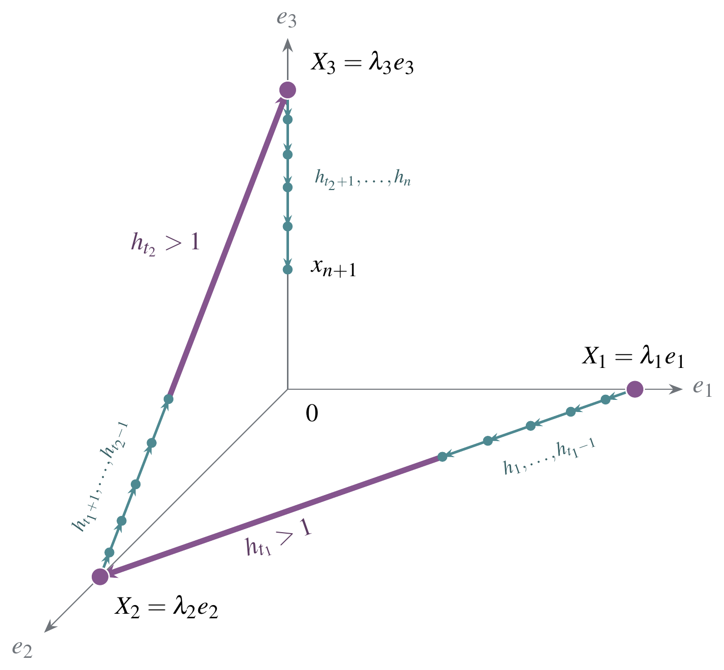
set $t_0=0$ and divide the schedule into $q$ transition blocks and one terminal block. For $1\le i\le q$, transition block $i$ contains $(h_{t_{i-1}+1}, \dots, h_{t_i})$, while the terminal block contains $(h_{t_q+1}, \dots, h_n)$. The construction first specifies a desirable trajectory. Place anchors

$ X_i=\lambda_i e_i, \qquad 1\le i\le q+1, $

where $e_1, \ldots, e_{q+1}$ are orthonormal. Then, for each $1\le i\le q$, arrange for the iterates to start at the anchor $X_i$, make only one-dimensional progress, and reach the next anchor $X_{i+1}$ at the final selected long step. As a consequence, the gradient $g_i$ for this block is fixed to be

$ g_i=\frac{X_{i}-X_{i+1}}{S_i+h_{t_i}}, \qquad 1\le i\le q. $

Note that after the final selected long step lands on the next coordinate-axis anchor $X_{i+1}$, the active gradient changes from $g_i$ to $g_{i+1}$. After the last selected step, the remaining iterates use

$ g_{q+1}=\frac{\lambda_{q+1}}{1+2S_{q+1}}e_{q+1}. $

Figure 5 illustrates this geometry.

Construction of the hard function via a Moreau envelope.

The remaining question is how to realize this prescribed piecewise-constant gradient pattern with one globally defined smooth convex function. Intuitively, this is possible by gluing Huber functions together. The selected long steps provide enough room for the landscape of the hard function to change while maintaining its smoothness.

More precisely, let

$ C:=\operatorname{conv}{0, g_1, \ldots, g_{q+1}}, $

and consider its support function

$ \sigma_C(z):=\max_{g\in C}\langle g, z\rangle. $

The support function stores the candidate block gradients as slopes. Now take the Moreau envelope of the support function $\sigma_C$,

$ f_C(x):= \min_z\left{\sigma_C(z)+\frac12\lVert x-z\rVert^2\right}. $

Since $\sigma_C$ is proper, closed, and convex, its Moreau envelope $f_C$ is convex and has a $1$-Lipschitz gradient ([29], Propositions 5.b, 7.b, and 7.d). The hard function $f_C$ satisfies the distance and projection identities ([2], Lemma 4.2)

$ f_C(x)=\frac12\lVert x\rVert^2-\frac12d(x, C)^2, \qquad \nabla f_C(x)=\Pi_C(x). $

Completing the square also gives

$ f_C(x)= \max_{g\in C}\left{\langle g, x\rangle-\frac12\lVert g\rVert^2\right}. $

This hard function can be regarded as a multidimensional analogue of the Huber function. On $C$ it equals $\frac12\lVert x\rVert^2$. On a normal-cone region where $\Pi_C(x)=g_i$, it equals $\langle g_i, x\rangle-\frac12\lVert g_i\rVert^2$ and is therefore affine. The trajectory stays in these constant-projection regions between selected long steps. In this sense, the construction retains the quadratic region $C$ and affine outer pieces of the one-dimensional Huber function while using new coordinate axes to keep the effects of several selected long steps separate.

Hence prescribing $g_i$ as the gradient throughout a block reduces to the geometric condition

$ g_i=\Pi_C(x) \quad\Longleftrightarrow\quad \langle x-g_i, v-g_i\rangle\le0 \quad\text{for every }v\in C. $

Since $C$ is the convex hull of finitely many generators, it is enough to check this inequality at $0, g_1, \ldots, g_{q+1}$. The proof in ([2], Theorem 4.1) parameterizes the positive scales by the amplitude ratios $\gamma_i:=\lambda_{i+1}/\lambda_i$. That theorem gives an explicit admissible upper bound for each $\gamma_i^2$. Choosing the ratios within these ranges ensures the projection inequalities along every intended block. Saturating the explicit upper bounds on $\gamma_i$ maximizes the final gap $f_C(x_{n+1})-f_C(0)$ and yields the lower bound in Lemma 3.

B. Properties of J(alpha, lambda) and Numerical Solution

The proofs of Theorem 1 and Theorem 2 reduce to finding the smallest possible $\alpha>0$ for which $J(\alpha, \lambda)\le0$ for some $\lambda>0$; see Equation 13–Equation 14.[^2] Accordingly, for each exponent parameter $\alpha$, we optimize over the scalar parameter $\lambda$ in Equation 12 and define

[^2]: For the anytime case, the inequality must be strict; see Equation 31–Equation 32.

$ \hat{J}(\alpha):=\inf_{\lambda>0}J(\alpha, \lambda).\tag{33} $

It remains to find the smallest $\alpha>0$ for which $\hat{J}(\alpha)\le0$. The following proposition gives the properties needed to determine $\alpha$ and $\lambda$.

########## {caption="Proposition 14"}

For every $\alpha>0$, the function $\lambda\mapsto J(\alpha, \lambda)$ is strictly convex and has a unique minimizer $\lambda_\star(\alpha)\in(1/4, 1/2)$. The function $\hat{J}$ is continuous and strictly decreasing. Hence it has a unique zero $\alpha_\star$ on every interval where it changes sign.

Proof: Let $u_\lambda=(x_\lambda, y_\lambda)$ be the optimizer defining $\Gamma_\lambda(w, z)$, and let $H$ be the Hessian of $\log K_{w, z}$ at $u_\lambda$. By Lemma 6, this optimizer is unique and $H$ is negative definite. Applying the implicit function theorem to the first-order condition $\nabla_{x, y}\log K_{w, z}(u_\lambda)=\lambda\mathbf 1$ shows that $u_\lambda$ is differentiable in $\lambda$ and that $u_\lambda'=H^{-1}\mathbf 1$. Differentiating the optimized value then gives

$ \begin{aligned} \partial_\lambda\Gamma_\lambda(w, z) &=-\mathbf 1^\top u_\lambda=-(x_\lambda+y_\lambda), \ \partial_{\lambda\lambda}\Gamma_\lambda(w, z) &=-\mathbf 1^\top H^{-1}\mathbf 1>0. \end{aligned} $

Consequently, $J(\alpha, \cdot)$ is strictly convex.

To determine the signs of $\partial_\lambda J$ at the endpoints $\lambda=1/4$ and $\lambda=1/2$, we need bounds on the optimizer $(x, y)$. Set $a:=x/(w+x)$ and $b:=y/(z+y)$. The first-order conditions give

$ \lambda(x+y) =1-\frac{(a-b)^2}{2(a+b-2ab)}. $

Since $a+b-2ab-(a-b)^2=a(1-a)+b(1-b)>0$, this identity yields $1/2<\lambda(x+y)\le1$. Equality in the upper bound forces $a=b$. Writing $\tau=x(w+x)/w=y(z+y)/z$, we have $w=\tau(1-a)^2/a$ and $z=\tau(1-b)^2/b$. Thus equality forces $w=z$. Therefore

$ \frac12<\lambda(x+y)\le1.\tag{34} $

Moreover, the upper bound is strict whenever $w\ne z$.

By Equation 34, $x+y\le1/\lambda$, so $|\partial_\lambda\Gamma_\lambda|$ has a uniform bound on every compact $\lambda$-interval. We may therefore differentiate under the integral in Equation 12 to obtain

$ \partial_\lambda J(\alpha, \lambda) =2-2\int_0^{1/2} \bigl(x_{\alpha, \lambda}(t)+y_{\alpha, \lambda}(t)\bigr), dt,\tag{35} $

where $(x_{\alpha, \lambda}(t), y_{\alpha, \lambda}(t))$ is the optimizer corresponding to $(w, z)=(W_\alpha(t), W_\alpha(1-t))$. It follows from Equation 35 that $\partial_\lambda J(\alpha, 1/4)<0$ and $\partial_\lambda J(\alpha, 1/2)>0$. The latter inequality is strict because equality in $\lambda(x+y)\le1$ can occur only when $w=z$, which here happens only at $t=1/2$. Thus the unique minimizer lies in $(1/4, 1/2)$.

For fixed $\lambda$, $W_\alpha(t)$ increases strictly with $\alpha$, while $\Gamma_\lambda$ decreases strictly in each coordinate. Therefore $J(\alpha, \lambda)$ decreases strictly with $\alpha$. If $0<\alpha_1<\alpha_2$, evaluating $J(\alpha_2, \cdot)$ at $\lambda_\star(\alpha_1)$ gives $\hat{J}(\alpha_2)<\hat{J}(\alpha_1)$.

It remains to prove continuity. The estimates in the proof of Lemma 9 are locally uniform in $(\alpha, \lambda)$. Consequently, the integrand in Equation 12 extends continuously to $t=0$, locally uniformly on compact parameter sets, and is locally bounded there. Together with the implicit-function argument above, dominated convergence shows that $J$ is jointly continuous. Since the minimizer always lies in the fixed compact interval $[1/4, 1/2]$, minimizing over that interval gives continuity of $\hat{J}$.

Numerical solution.

For $u, \tau>0$, write

$ X_u(\tau):=\frac{2\tau}{1+\sqrt{1+4\tau/u}} =f_u(\tau)-u. $

For fixed $\alpha, \lambda>0$ and $0<t\le1/2$, put $w=W_\alpha(t)$ and $z=W_\alpha(1-t)$. The optimizer defining $\Gamma_\lambda(w, z)$ is $x=X_w(\tau)$ and $y=X_z(\tau)$, where $\tau$ is the unique root of Equation 21. At $t=0$, we use the continuous extension established above. At this root,

$ \Gamma_\lambda(w, z) =\log\left[\tau\left(\frac1{f_w(\tau)}+\frac1{f_z(\tau)}\right) \right] -\lambda\bigl(X_w(\tau)+X_z(\tau)\bigr).\tag{36} $

To evaluate $J(\alpha, \lambda)$ and $\partial_\lambda J(\alpha, \lambda)$, we solve Equation 21 at each quadrature node and use Equation 36 and 35. For fixed $\alpha$, $\partial_\lambda J(\alpha, \cdot)$ is continuous and strictly increasing and has opposite signs at $1/4$ and $1/2$. Bisection therefore gives $\lambda_\star(\alpha)$. A second bisection applied to the continuous, strictly decreasing function $\hat{J}$ gives its zero $\alpha_\star$.

Floating-point computation gives

$ \alpha_\star\approx0.63416058454, \qquad \lambda_\star(\alpha_\star)\approx0.45060731.\tag{37} $

These digits describe the optimized pair but are not used as a rigorous certificate. The proof uses the nearby pair $(\alpha, \lambda)=(0.6342, 0.4506)$. A computer-assisted calculation using Arb with directed outward rounding certifies

$ J(0.6342, 0.4506)<-0.0000512188<-0.00005<0,\tag{38} $

which is the inequality used in the proofs of Theorem 1 and Theorem 2.

C. Proofs for the Anytime Lower Bound

This appendix proves Lemma 10 and Lemma 11.

C.1 Proof and Intuition of Lemma 10

We first explain how the proof of Lemma 10 modifies the finite-to-anytime transfer of ([3], Theorem 4.1). We begin with two lower bounds from one-dimensional hard instances that drive this transfer. For a prefix $H_n=(h_1, \ldots, h_n)$, the first one relates $R_n(H_n)$ to the total stepsize $h_{1:n}$ . Using convex quadratics, ([3], Lemma 2.1) gives

$ R_n(H_n)\ge\frac{1}{4(1+2h_{1:n})}.\tag{39} $

We instead use the standard Huber loss from Fact 12, which gives the stronger bound $R_n(H_n)\ge \frac{1}{1+2h_{1:n}}$, as stated in Equation 2. In particular, if $R_n(H_n)=o(n^{-p})$ for some $p>1$, then $h_{1:n}/n\to\infty$, and the stepsizes are unbounded.

The second bound comes from ([3], Lemma 3.1). Its hard instance is the asymmetric Huber loss

$ \psi_{\varepsilon, \delta}(u):= \begin{cases} \delta u-\delta^2/2, & u\ge\delta, \ u^2/2, & -\varepsilon\le u\le\delta, \ -\varepsilon u-\varepsilon^2/2, & u\le-\varepsilon. \end{cases}\tag{40} $

It is quadratic near the origin and affine on either side. By choosing $\varepsilon$ and $\delta$ so that the update with $h_m>1$ crosses the quadratic region, their lemma proves

$ R_n(H_n)\ge \frac{(h_m-1)^2} {(1+h_{1:m-1})^2(1+2h_{m+1:n})}.\tag{41} $

We only use the case $m=n$, which gives

$ h_n-1\le(1+h_{1:n-1})\sqrt{R_n(H_n)} \qquad\text{when }h_n>1.\tag{42} $

The proof of the $\Omega(n^{-4/3})$ anytime lower bound in ([3], Theorem 4.1) combines Equation 39, Equation 41, and their Lemmas 2.2 and 2.3. The latter use convex quadratics to control the total stepsize through the largest stepsize. Figure 6 summarizes their argument.

Our proof uses the stronger total-sum bound Equation 2 in place of ([3], Lemma 2.1), retains the terminal-step bound Equation 42 from ([3], Lemma 3.1), and replaces the use of ([3], Lemmas 2.2 and 2.3) with the two more refined tail bounds in Equation 43, valid for every $m$ such that $R_n(H)D_m\le c_0$ . The proof of these tail bounds uses the same hard function and variable substitution as the proof of Lemma 4.

Proof of Lemma 10: Fix $\alpha>0$, and assume that Equation 28 implies Equation 29, with the same constants $\eta_\alpha, C_\alpha$ for every integer $q\ge 2$ and every integer $1\le \ell\le \eta_\alpha q$ .

Fix a finite schedule $H=(h_1, \ldots, h_n)$ . Recall the notation from Section 3.1. Let $a_1\ge\cdots\ge a_r>0$ be the decreasing rearrangement of the positive excesses $(h_k-1)_+$, and define

$ B:=1+\sum_{k=1}^n\min{h_k, 1}, \qquad D_s:=B+\sum_{j=s+1}^r a_j, \qquad 1\le s\le r. $

Part I: Constructing tail bounds.

We first prove that there are constants $c_0, C>0$, depending only on $\alpha$, such that any $1\le m\le r$ satisfying $R_n(H)D_m\le c_0$ also satisfies

$ m a_m\le C D_m, \qquad D_m\le C(n+1)^{1+\alpha}m^{-\alpha}.\tag{43} $

Together, these two bounds play the role of ([3], Lemmas 2.2 and 2.3) in our proof. The condition $R_n(H)D_m\le c_0$ implies $D_m\le c_0/R_n(H)$ . The first inequality compares $D_{m-1}$ and $D_m$, since $D_{m-1}=D_m+a_m\le(1+C/m)D_m$, while the second controls $D_m$ itself. Applying both bounds with $m=j$ gives $a_j\le C(n+1)^{1+\alpha}j^{-1-\alpha}$, whose sum controls the remaining smaller excesses.

We now prove the two inequalities in Equation 43. Note that only the proof of the second inequality uses the hypothesis that Equation 28 implies Equation 29. If $r=0$, there is nothing to prove. We may therefore assume $r\ge1$ . For the moment, let $c_0>0$, and let $m$ be arbitrary such that $R_n(H)D_m\le c_0$ . We collect the required restrictions on $c_0$ at the end of Part I. The $q=1$ case in the proof of Lemma 4 gives $R_n(H)D_1\ge1/4$ . Under the restriction $c_0<1/4$, the case $m=1$ cannot satisfy $R_n(H)D_m\le c_0$ . We henceforth consider only $2\le m\le r$ .

Fix $2\le q\le r$ . Following the notation in the proof of Lemma 4, let $t_1<\cdots<t_q$ be the locations of the $q$ largest positive excesses, with $t_0=0$ and $t_{q+1}=n+1$ . For $1\le i\le q+1$, set $S_i:=h_{t_{i-1}+1:t_i-1}$; for $1\le i\le q$, define

$ x_i:=\frac{q(S_i+1)}{D_q}, \qquad \omega_i:=\frac{q(h_{t_i}-1)}{D_q}, \qquad 1\le i\le q, $

with $\sum_{i=1}^q x_i<q$. Let $G$ be the right-hand side of Equation 1 for these selected indices. Then Lemma 3 gives $R_n(H)\ge G$, and 17 yields

$ R_n(H)\ge \frac{q}{D_q E_{\mathrm{end}} \prod_{i=1}^{q-1}K_{\omega_i, \omega_{i+1}}(x_i, x_{i+1})},\tag{44} $

Step 1. Prove the first inequality in Equation 43. Set $\beta_\alpha:=1+\max{e, \alpha}$ . We claim that

$ s a_s\le \beta_\alpha D_s, \qquad m\le s\le r.\tag{45} $

For every $m\le s\le r$, we have $D_s\le D_m$, and hence $R_n(H)D_s\le c_0$ . Apply Equation 44 with $q=s$ and use the $s$ largest excesses to form $x_1, \ldots, x_s$ and $\omega_1, \ldots, \omega_s$ . Every selected excess is at least $a_s$, so $\omega_i\ge s a_s/D_s$ for every $1\le i\le s$ .

If $s a_s>\beta_\alpha D_s$, then $\omega_i>\beta_\alpha$ for every $i$ . Define $\Gamma_1$ [^3] by

[^3]: Here $\Gamma_1=\left.\Gamma_\lambda\right|_{\lambda=1}$ .

$ \Gamma_1(w, z):= \sup_{x, y>0}{\log K_{w, z}(x, y)-(x+y)}. $

For the $x_i, \omega_i$ just obtained with $q=s$, put $\Delta_s:=s-\sum_{i=1}^s x_i>0$ . Since $\min_i\omega_i>\beta_\alpha$, the endpoint estimate in the proof of Lemma 5 gives

$ E_{\mathrm{end}}e^{-(2\Delta_s+x_1+x_s)} \le A_{\beta_\alpha},\tag{46} $

for some $A_{\beta_\alpha}<\infty$ depending only on $\beta_\alpha$ . Combining Equation 46 with the definition of $\Gamma_1$ gives

$ E_{\mathrm{end}} \prod_{i=1}^{s-1}K_{\omega_i, \omega_{i+1}}(x_i, x_{i+1}) \le A_{\beta_\alpha}\exp!\left{ 2s+\sum_{i=1}^{s-1}\Gamma_1(\omega_i, \omega_{i+1}) \right}. $

Because $\Gamma_1$ decreases in each coordinate and $\Gamma_1(\beta_\alpha, \beta_\alpha)=-\log\beta_\alpha-1$,

$ 2s+\sum_{i=1}^{s-1}\Gamma_1(\omega_i, \omega_{i+1}) \le 2s+(s-1)(-\log\beta_\alpha-1). $

Put $\delta:=\log\beta_\alpha-1>0$ . Then $2s+(s-1)(-\log\beta_\alpha-1)=-\delta s+\log\beta_\alpha+1$. The preceding product is therefore at most $\widetilde{A}{\beta\alpha}e^{-\delta s}$, where $\widetilde{A}{\beta\alpha}:=e\beta_\alpha A_{\beta_\alpha}$ . Applying Equation 44 with $q=s$ gives

$ R_n(H) \ge\frac{s}{D_s E_{\mathrm{end}} \prod_{i=1}^{s-1}K_{\omega_i, \omega_{i+1}}(x_i, x_{i+1})} \ge\frac{s e^{\delta s}}{\widetilde{A}{\beta\alpha}D_s} \ge\frac{s e^{\delta s}}{\widetilde{A}{\beta\alpha}c_0}R_n(H), $

If $\widetilde{A}{\beta\alpha}c_0<1$, then $s\ge m\ge2$ gives $s e^{\delta s}/(\widetilde{A}_{\beta_\alpha}c_0)>1$, a contradiction. Hence Equation 45, and thus the first inequality in Equation 43, holds under this condition.

Step 2. Prove the second inequality in Equation 43.

Assume $\widetilde{A}{\beta\alpha}c_0<1$, so that Step 1 applies. Put $F_s:=D_s s^\alpha$, and choose

$ \widehat{q}\in\operatorname*{arg, min}_{m\le s\le r}F_s. $

Using Equation 45, $D_{s-1}=D_s+a_s$, and $\log(1+u)\le u$, we obtain, for every $m<q\le r$,

$ \log\frac{D_m}{D_q} =\sum_{s=m+1}^q\log\left(1+\frac{a_s}{D_s}\right) \le \beta_\alpha\sum_{s=m+1}^q\frac1s \le \beta_\alpha\log\frac qm. $

Therefore

$ \frac{D_q}{D_m}\ge\left(\frac mq\right)^{\beta_\alpha}. $

We now prove that $F_m\le A F_r$ for a constant $A$ depending only on $\alpha$ . Take $A\ge\eta_\alpha^{-(\beta_\alpha-\alpha)}$ . If $F_m>A F_r$, then $\widehat{q}>m$ and

$ \frac{F_{\widehat{q}}}{F_m}<\frac1A, \qquad \frac{F_{\widehat{q}}}{F_m} =\frac{D_{\widehat{q}}}{D_m} \left(\frac{\widehat{q}}{m}\right)^\alpha \ge\left(\frac m{\widehat{q}}\right)^{\beta_\alpha-\alpha}. $

Hence $m/\widehat{q}<A^{-1/(\beta_\alpha-\alpha)}\le\eta_\alpha$, so $m<\eta_\alpha\widehat{q}$ . Because the selected excesses are $a_1, \ldots, a_{\widehat{q}}$, the decreasing rearrangement of the normalized weights satisfies $\omega_j^\downarrow=\widehat{q} a_j/D_{\widehat{q}}$ for $1\le j\le\widehat{q}$ . For every $m\le k<\widehat{q}$, the minimizing property of $\widehat{q}$ gives

$ \sum_{s=k+1}^{\widehat{q}}\omega_s^\downarrow =\frac{\widehat{q}}{D_{\widehat{q}}} \sum_{s=k+1}^{\widehat{q}}a_s =\widehat{q}\left(\frac{D_k}{D_{\widehat{q}}}-1\right) \ge \widehat{q} \left[\left(\frac{\widehat{q}}{k}\right)^\alpha-1\right].\tag{47} $

This inequality, $m\le\eta_\alpha\widehat{q}$, and the bound $\sum_{i=1}^{\widehat{q}}x_i<\widehat{q}$ together verify Equation 28 with $q=\widehat{q}$ and $\ell=m$ . Applying Equation 29 gives

$ E_{\mathrm{end}} \prod_{i=1}^{\widehat{q}-1} K_{\omega_i, \omega_{i+1}}(x_i, x_{i+1}) \le C_\alpha. $

Combining this estimate with Equation 44 and $D_{\widehat{q}}\le D_m\le c_0/R_n(H)$ gives

$ R_n(H)\ge\frac{\widehat{q}}{C_\alpha D_{\widehat{q}}} \ge\frac{\widehat{q}}{C_\alpha c_0}R_n(H), $

If, in addition, $C_\alpha c_0<1$, then $\widehat{q}/(C_\alpha c_0)>1$, a contradiction. Hence $F_m\le A F_r$ under these conditions. Since $D_r=B\le n+1$ and $r\le n$,

$ D_m m^\alpha=F_m \le A F_r =A D_r r^\alpha \le A(n+1)n^\alpha. $

Collecting the conditions used above, choose, once and for all,

$ 0<c_0< \min\left{ \frac14, \widetilde{A}{\beta\alpha}^{-1}, C_\alpha^{-1} \right}. $

For this choice, the preceding argument proves both inequalities in Equation 43 for every $m$ satisfying $R_n(H)D_m\le c_0$ . Since $\beta_\alpha, \widetilde{A}{\beta\alpha}, C_\alpha$, and $A$ depend only on $\alpha$, so does $c_0$ . Taking $C:=\max{\beta_\alpha, A}$ completes Part I.

Part II: The anytime transfer.

We now combine Part I with Equation 2 and 42. The remaining proof adapts the finite-to-anytime transfer in ([3], Proof of Theorem 4.1). Fix a positive infinite schedule. For each prefix $H_n$, define $a_1, \ldots, a_r, B, D_s$ as in Part I.

Suppose for contradiction that

$ R_n(H_n)=o!\left(n^{-2(1+\alpha)/(2+\alpha)}\right). $

Since $\alpha>0$, the exponent $2(1+\alpha)/(2+\alpha)$ is greater than $1$ . The contradiction hypothesis and 2 therefore imply $h_{1:n}/n\to\infty$ . Hence the stepsizes are unbounded, and there are arbitrarily large indices $n$ satisfying

$ h_n=\max_{1\le k\le n}h_k>1.\tag{48} $

Moreover, since $D_r=B\le n+1$,

$ R_n(H_n)D_r \le (n+1)R_n(H_n) =o!\left(n^{-\alpha/(2+\alpha)}\right) \longrightarrow 0. $

We may therefore fix one such $n$, sufficiently large that both Equation 48 and $R_n(H_n)D_r\le c_0$ hold. Since $h_n$ is the largest stepsize in $H_n$, its excess is the largest, and hence $a_1=h_n-1$ .

Define the cutoff[^4]

[^4]: We explain the choice of $m_\star$ in Remark 15.

$ m_\star:=\left\lfloor \frac{1}{4\sqrt{R_n(H_n)}} \right\rfloor.\tag{49} $

Since $R_n(H_n)\to0$ and $\lfloor x\rfloor\ge x/2$ for $x\ge2$, our sufficiently large choice of $n$ satisfies

$ m_\star\ge\frac{1}{8\sqrt{R_n(H_n)}}.\tag{50} $

If the number of long steps $r\le m_\star$, the terminal-step bound Equation 42 gives

$ \sum_{j=1}^r a_j \le m_\star a_1 \le\frac14(1+h_{1:n}). $

Since $h_{1:n}=(B-1)+\sum_{j=1}^r a_j$ and $B-1\le n$, this would imply $h_{1:n}=O(n)$, a contradiction. Thus $r>m_\star$ .

To apply Part I with $m=m_\star$, we first prove that $R_n(H_n)D_{m_\star}\le c_0$ . Suppose instead that $R_n(H_n)D_{m_\star}>c_0$ . Since $r>m_\star$, $R_n(H_n)D_r\le c_0$, and $D_s$ decreases with $s$, there is a smallest index $q_\star>m_\star$ such that

$ R_n(H_n)D_{q_\star}\le c_0. $

Applying both inequalities in Equation 43 with $m=q_\star$ gives

$ D_{q_\star-1}=D_{q_\star}+a_{q_\star} \le\left(1+\frac C{q_\star}\right)D_{q_\star} \le C(n+1)^{1+\alpha}q_\star^{-\alpha}. $

Using $q_\star>m_\star$ and 50, we obtain

$ \begin{aligned} R_n(H_n)D_{q_\star-1} &\le C n^{1+\alpha}R_n(H_n)^{1+\alpha/2}\ &=C\left(n^{\frac{2(1+\alpha)}{2+\alpha}}R_n(H_n) \right)^{(2+\alpha)/2} =o(1), \end{aligned} $

contradicting the minimality of $q_\star$, which gives $R_n(H_n)D_{q_\star-1}>c_0$ . Hence

$ R_n(H_n)D_{m_\star}\le c_0.\tag{51} $

For every $m_\star<j\le r$, $D_j\le D_{m_\star}$, so $R_n(H_n)D_j\le c_0$ . Applying Equation 43 with $m=j$ gives

$ a_j\le\frac{C D_j}{j} \le C(n+1)^{1+\alpha}j^{-1-\alpha}. $

For $1\le j\le m_\star$, we have $a_j\le a_1=h_n-1$, so the terminal-step bound Equation 42 controls the first sum below. For $m_\star<j\le r$, sum the preceding estimate and use Equation 50 for the second sum:

$ \begin{aligned} \sum_{j=1}^{m_\star}a_j &\le m_\star a_1 \le\frac14(1+h_{1:n}), \ \sum_{j=m_\star+1}^{r}a_j &\le C(n+1)^{1+\alpha} \sum_{j=m_\star+1}^{\infty}j^{-1-\alpha}\ &\le C(n+1)^{1+\alpha}m_\star^{-\alpha} \le C(n+1)^{1+\alpha}R_n(H_n)^{\alpha/2}. \end{aligned} $

Using $h_{1:n}=(B-1)+\sum_j a_j$ and $B-1\le n$, we absorb $\tfrac14 h_{1:n}$ into the left-hand side to obtain

$ h_{1:n}\le C\left(n+n^{1+\alpha}R_n(H_n)^{\alpha/2}\right).\tag{52} $

Multiplying by $R_n(H_n)$ gives

$ \begin{aligned} R_n(H_n)h_{1:n} &\le C\left(nR_n(H_n)+n^{1+\alpha}R_n(H_n)^{1+\alpha/2} \right)\ &=C\left(nR_n(H_n)+ \left(n^{\frac{2(1+\alpha)}{2+\alpha}}R_n(H_n)\right)^{(2+\alpha)/2} \right) =o(1). \end{aligned} $

But Equation 2 gives $R_n(H_n)(1+2h_{1:n})\ge1$, a contradiction. Therefore

$ \limsup_{n\to\infty} n^{\frac{2(1+\alpha)}{2+\alpha}}R_n(H_n)>0. $

########## {caption="Remark 15"}

We explain the choice of $m_\star$ in Equation 49. For the chosen $n$, $h_n=\max_{1\le k\le n}h_k>1$, so $a_1=h_n-1$ . The terminal-step bound Equation 42 gives $a_1\le(1+h_{1:n})\sqrt{R_n(H_n)}$. Since $a_j\le a_1$, every cutoff $m$ satisfies

$ \sum_{j=1}^{m}a_j \le m(1+h_{1:n})\sqrt{R_n(H_n)}. $

The head estimate only requires $m_\star\le \varepsilon R_n(H_n)^{-1/2}$, where $\varepsilon\in(0, 1)$ is fixed. Indeed, the preceding inequality then gives $\sum_{j=1}^{m_\star}a_j\le\varepsilon(1+h_{1:n})$, which can be absorbed in Equation 52 since $\varepsilon<1$ . In Equation 49, we take $\varepsilon=1/4$ . Part I then gives

$ \sum_{j>m_\star}a_j \le C(n+1)^{1+\alpha}m_\star^{-\alpha} \le C(n+1)^{1+\alpha}R_n(H_n)^{\alpha/2}. $

Combining the head and tail estimates with $h_{1:n}=(B-1)+\sum_{j\le m_\star}a_j+\sum_{j>m_\star}a_j$ recovers Equation 52.

C.2 Proof of Lemma 11

We adapt the proof of Lemma 7 to establish Equation 30.

Proof:

Step 1. Eliminate the $x_i$ 's.

Taking $k=q-1$ in Equation 28 gives $\min_i\omega_i\ge\alpha$, the only consequence of the tail conditions used in the proof of Lemma 5. Hence the same proof gives

$ E_{\mathrm{end}} \prod_{i=1}^{q-1}K_{\omega_i, \omega_{i+1}}(x_i, x_{i+1}) \le C_{\alpha, \lambda} \exp!\left{ 2\lambda q+ \sum_{i=1}^{q-1}\Gamma_\lambda(\omega_i, \omega_{i+1}) \right}. $

It remains to bound the sum in the exponent.

Step 2. Set aside the $\ell$ unconstrained largest weights.

We first split the consecutive-pair sum from Step 1 into an odd matching and an even matching, according to whether $i$ is odd or even.

$ (\omega_1, \omega_2), (\omega_3, \omega_4), \ldots \qquad\text{and}\qquad (\omega_2, \omega_3), (\omega_4, \omega_5), \ldots. $

The tail inequalities in Equation 28 do not constrain the $\ell$ largest weights $\omega_1^\downarrow, \ldots, \omega_\ell^\downarrow$ . Mark their positions in the chronological sequence and delete, from each matching, every pair containing one of these positions. Each marked position belongs to at most one pair in each matching, so at most $2\ell$ terms are deleted in total.

Let $M_0$ and $M_1$ denote the remaining odd and even matchings, respectively, and put

$ k_\nu:=|M_\nu|, \qquad d_\nu:=q-2k_\nu. $

Thus $d_\nu$ is the number of positions not used by $M_\nu$ . Since $M_\nu$ contains none of the $\ell$ marked positions, $d_\nu\ge\ell$ . Before any pair is deleted, each of the odd and even matchings leaves at most two positions unused. Deleting a pair creates two additional unused positions, and at most $\ell$ pairs are deleted from either matching. Hence

$ \ell\le d_\nu\le2\ell+2.\tag{53} $

Recall the comparison weights $\bar{w}_s^{(q)}$ from Equation 23. They satisfy $\bar{w}_q^{(q)}\le\cdots\le\bar{w}_2^{(q)}$ and, for every $\ell\le m<q$,

$ \sum_{s=m+1}^q\bar{w}_s^{(q)} =q\left[\left(\frac qm\right)^\alpha-1\right]. $

Hence Equation 28 gives, for every $1\le j\le q-\ell$,

$ \sum_{s=q-j+1}^q\omega_s^\downarrow \ge \sum_{s=q-j+1}^q\bar{w}_s^{(q)}.\tag{54} $

Step 3. Identify the maximizing matching and compare it with the integral.

After ordering the remaining weights increasingly, each $M_\nu$ is a $k_\nu$ -edge matching on $(\omega_q^\downarrow, \ldots, \omega_{\ell+1}^\downarrow)$ . The proof of Lemma 7 shows that $\Phi_{k_\nu, \lambda}$ is symmetric, convex, and coordinatewise decreasing. Hence Lemma 8, Equation 54, and 25 give, for $\nu\in{0, 1}$,

$ \begin{aligned}\sum_{{i, j}\in M_\nu} \Gamma_\lambda(\omega_i, \omega_j) &\le \Phi_{k_\nu, \lambda} (\omega_q^\downarrow, \ldots, \omega_{\ell+1}^\downarrow)\&\le \Phi_{k_\nu, \lambda} (\bar{w}q^{(q)}, \ldots, \bar{w}{\ell+1}^{(q)})\&= \sum_{j=1}^{k_\nu}\Gamma_\lambda!\left(\bar{w}{q+1-j}^{(q)}, \bar{w}{d_\nu+j}^{(q)} \right).\end{aligned}\tag{55} $

We next compare the explicit matching sum in Equation 55 with its corresponding Riemann integral. Recall that $W_\alpha(t)=\alpha t^{-1-\alpha}$ for $0<t\le1$ . By Lemma 9,

$ g_{\alpha, \lambda}(t) :=\Gamma_\lambda(W_\alpha(t), W_\alpha(1-t)), \qquad 0<t\le\frac12, $

extends continuously to $t=0$ . Define

$ I_{\alpha, \lambda} :=\int_0^{1/2}g_{\alpha, \lambda}(t), dt. $

We use the following shifted Riemann-sum estimate. For every integer $0\le k\le\lfloor(q-1)/2\rfloor$, set $d:=q-2k$, so $d\ge1$ . Then

$ \sum_{j=1}^{k} \Gamma_\lambda!\left(\bar{w}{q+1-j}^{(q)}, \bar{w}{d+j}^{(q)} \right) \le qI_{\alpha, \lambda}+C_{\alpha, \lambda}(d+1).\tag{56} $

Set $M_{\alpha, \lambda}:=\max{0, \Gamma_\lambda(\alpha, \alpha)}$ . To prove Equation 56, first suppose $d\ge q/4$ . Since every $\bar{w}s^{(q)}\ge\alpha$, each summand is at most $M{\alpha, \lambda}$ . Therefore

$ \sum_{j=1}^{k} \Gamma_\lambda(\bar{w}{q+1-j}^{(q)}, \bar{w}{d+j}^{(q)}) -qI_{\alpha, \lambda} \le q\left(\frac{M_{\alpha, \lambda}}2+|I_{\alpha, \lambda}|\right) \le C_{\alpha, \lambda}d. $

Now suppose $d<q/4$ . By the mean-value theorem, for each $2\le s\le q$, there is $\xi_s\in(s-1, s)$ such that

$ \bar{w}s^{(q)}=W\alpha(\xi_s/q). $

The Lipschitz estimate in Lemma 9 applies to $(u, v)\mapsto\Gamma_\lambda(W_\alpha(u), W_\alpha(v))$ on $[0, 1/2]\times[1/2, 1]$ .

For each $j$ such that $u_j:=(d+j)/q\le1/2$,

$ \left|\frac{\xi_{d+j}}q-u_j\right|\le\frac1q, \qquad \left|\frac{\xi_{q+1-j}}q-(1-u_j)\right| \le\frac{d+1}{q}. $

Symmetry and the Lipschitz estimate give

$ \Gamma_\lambda!\left(\bar{w}{q+1-j}^{(q)}, \bar{w}{d+j}^{(q)} \right) \le g_{\alpha, \lambda}(u_j) +C_{\alpha, \lambda}\frac{d+1}{q}. $

Since $1\le j\le k=(q-d)/2$, there are at most $d+1$ indices with $u_j>1/2$ . For these indices, both $\xi_{d+j}/q$ and $\xi_{q+1-j}/q$ lie in $[1/4, 1]$, because $d<q/4$ . Thus both arguments of $\Gamma_\lambda$ lie in $[\alpha, \alpha, 4^{1+\alpha}]$, and the total contribution of these terms is at most $C_{\alpha, \lambda}(d+1)$ . For the other indices, the grid $u_j$ has mesh $1/q$ and begins at $(d+1)/q$ . The portion of $[0, 1/2]$ not covered by the corresponding Riemann cells has total length at most $(d+1)/q$ . The boundedness and Lipschitz continuity of $g_{\alpha, \lambda}$ therefore give

$ \sum_{j:, u_j\le1/2}g_{\alpha, \lambda}(u_j) \le qI_{\alpha, \lambda}+C_{\alpha, \lambda}(d+1). $

Summing the error $C_{\alpha, \lambda}(d+1)/q$ over these indices and adding the at most $d+1$ terms with $u_j>1/2$ proves Equation 56.

Apply Equation 56 to the odd and even matchings $M_0$ and $M_1$, with $(k, d)=(k_\nu, d_\nu)$ . Add back the at most $2\ell$ terms deleted in Step 2. Since $\omega_i\ge\alpha$ for every $i$ by Step 1, each deleted term is at most $M_{\alpha, \lambda}$ . Since $d_\nu\le2\ell+2$, we obtain

$ \sum_{i=1}^{q-1}\Gamma_\lambda(\omega_i, \omega_{i+1}) \le 2qI_{\alpha, \lambda} +C_{\alpha, \lambda}(\ell+1).\tag{57} $

Combining the estimate from Step 1 with Equation 57 and using $J(\alpha, \lambda)=2\lambda+2I_{\alpha, \lambda}$ from Equation 12 proves Equation 30.

References

Section Summary: This section is a bibliography of 23 sources that the paper draws upon, spanning foundational works from the 1800s and mid-20th century through recent research papers and preprints. The listed items focus on mathematical techniques for improving the speed and efficiency of iterative algorithms used to solve optimization problems. They include both classic textbooks and new studies examining performance limits, step-size choices, and convergence behavior in gradient-based methods.

[1] Nemirovsky, Arkadii S. and Yudin, David B. (1983). Problem Complexity and Method Efficiency in Optimization. John Wiley & Sons.

[2] Ma, Jianhao and Chen, Yuxin (2026). A lower bound for stepsize-based acceleration of gradient descent. arXiv preprint arXiv:2608.10418. doi:10.48550/arXiv.2608.10418. https://arxiv.org/abs/2608.10418.

[3] Tsai et al. (2026). Lower Bounds for Anytime Acceleration of Gradient Descent. arXiv preprint arXiv:2607.02053. doi:10.48550/arXiv.2607.02053. https://arxiv.org/abs/2607.02053.

[4] Altschuler, Jason M. and Parrilo, Pablo A. (2025). Acceleration by stepsize hedging: Silver Stepsize Schedule for smooth convex optimization. Mathematical Programming. 213(1–2). pp. 1105–1118. doi:10.1007/s10107-024-02164-2. https://doi.org/10.1007/s10107-024-02164-2. arXiv:2309.16530.

[5] Grimmer et al. (2025). Composing Optimized Stepsize Schedules for Gradient Descent. Mathematics of Operations Research. doi:10.1287/moor.2024.0764. https://doi.org/10.1287/moor.2024.0764. arXiv:2410.16249.

[6] Cauchy, Augustin-Louis (1847). Méthode générale pour la résolution des systèmes d'équations simultanées. Comptes Rendus Hebdomadaires des Séances de l'Académie des Sciences. 25. pp. 536–538. https://gallica.bnf.fr/ark:/12148/bpt6k2982c/f540.item.

[7] Levitin, E. S. and Polyak, B. T. (1966). Constrained Minimization Methods. USSR Computational Mathematics and Mathematical Physics. 6(5). pp. 1–50. doi:10.1016/0041-5553(66)90114-5. https://doi.org/10.1016/0041-5553(66)90114-5.

[8] Nesterov, Yurii (2004). Introductory Lectures on Convex Optimization: A Basic Course. Kluwer Academic Publishers. doi:10.1007/978-1-4419-8853-9. https://doi.org/10.1007/978-1-4419-8853-9.

[9] Polyak, Boris T. (1964). Some Methods of Speeding Up the Convergence of Iteration Methods. USSR Computational Mathematics and Mathematical Physics. 4(5). pp. 1–17. doi:10.1016/0041-5553(64)90137-5. https://doi.org/10.1016/0041-5553(64)90137-5.

[10] Nesterov, Yurii E. (1983). A Method of Solving a Convex Programming Problem with Convergence Rate $O(1/k^2)$. Soviet Mathematics Doklady. 27(2). pp. 372–376.

[11] Grimmer, Benjamin (2024). Provably Faster Gradient Descent via Long Steps. SIAM Journal on Optimization. 34(3). pp. 2588–2608. doi:10.1137/23M1588408. https://doi.org/10.1137/23M1588408. arXiv:2307.06324.

[12] Grimmer et al. (2025). Accelerated Objective Gap and Gradient Norm Convergence for Gradient Descent via Long Steps. INFORMS Journal on Optimization. 7(2). pp. 156–169. doi:10.1287/ijoo.2024.0057. https://doi.org/10.1287/ijoo.2024.0057. arXiv:2403.14045.

[13] Zhang et al. (2025). Anytime Acceleration of Gradient Descent. In Proceedings of Thirty Eighth Conference on Learning Theory. pp. 5991–6013. https://proceedings.mlr.press/v291/zhang25a.html.

[14] Tsai, Chung-En (2026). An Improved Lower Bound for Non-Anytime Gradient Descent. Blog post, https://chungentsai.github.io/gd-lower-bounds.html. https://chungentsai.github.io/gd-lower-bounds.html.

[15] Drori, Yoel and Teboulle, Marc (2014). Performance of First-Order Methods for Smooth Convex Minimization: A Novel Approach. Mathematical Programming. 145(1–2). pp. 451–482. doi:10.1007/s10107-013-0653-0. https://doi.org/10.1007/s10107-013-0653-0.

[16] Taylor et al. (2017). Smooth Strongly Convex Interpolation and Exact Worst-Case Performance of First-Order Methods. Mathematical Programming. 161(1–2). pp. 307–345. doi:10.1007/s10107-016-1009-3. https://doi.org/10.1007/s10107-016-1009-3. arXiv:1502.05666.

[17] Das Gupta et al. (2024). Branch-and-Bound Performance Estimation Programming: A Unified Methodology for Constructing Optimal Optimization Methods. Mathematical Programming. 204(1–2). pp. 567–639. doi:10.1007/s10107-023-01973-1. https://doi.org/10.1007/s10107-023-01973-1. arXiv:2203.07305.

[18] Kamri et al. (2025). Numerical Design of Optimized First-Order Algorithms. arXiv preprint arXiv:2507.20773. doi:10.48550/arXiv.2507.20773. https://arxiv.org/abs/2507.20773.

[19] Teboulle, Marc and Vaisbourd, Yakov (2023). An Elementary Approach to Tight Worst Case Complexity Analysis of Gradient Based Methods. Mathematical Programming. 201(1–2). pp. 63–96. doi:10.1007/s10107-022-01899-0. https://doi.org/10.1007/s10107-022-01899-0.

[20] Young, David (1953). On Richardson's Method for Solving Linear Systems with Positive Definite Matrices. Journal of Mathematics and Physics. 32(1–4). pp. 243–255. doi:10.1002/sapm1953321243. https://doi.org/10.1002/sapm1953321243.

[21] Agarwal et al. (2021). Acceleration via Fractal Learning Rate Schedules. In Proceedings of the 38th International Conference on Machine Learning. pp. 87–99. https://proceedings.mlr.press/v139/agarwal21a.html.

[22] Zhang, Zehao and Jiang, Rujun (2026). Accelerated Gradient Descent by Concatenation of Stepsize Schedules. SIAM Journal on Optimization. 36(2). pp. 1182–1210. doi:10.1137/25M173898X. https://doi.org/10.1137/25M173898X.

[23] Kornowski, Guy and Shamir, Ohad (2024). Open Problem: Anytime Convergence Rate of Gradient Descent. In Proceedings of the Thirty-Seventh Conference on Learning Theory. pp. 5335–5339. https://proceedings.mlr.press/v247/kornowski24a.html.

[24] Bok, Jinho and Altschuler, Jason M. (2025). Accelerating Proximal Gradient Descent via Silver Stepsizes. In Proceedings of the Thirty-Eighth Conference on Learning Theory. pp. 421–453. https://proceedings.mlr.press/v291/bok25a.html.

[25] Altschuler, Jason M. and Parrilo, Pablo A. (2025). Acceleration by Stepsize Hedging: Multi-Step Descent and the Silver Stepsize Schedule. Journal of the ACM. 72(2). pp. 1–38. doi:10.1145/3708502. https://doi.org/10.1145/3708502.

[26] Arjevani, Yossi and Shamir, Ohad (2016). On the Iteration Complexity of Oblivious First-Order Optimization Algorithms. In Proceedings of the 33rd International Conference on Machine Learning. pp. 908–916. https://proceedings.mlr.press/v48/arjevani16.html.

[27] Marshall et al. (2011). Inequalities: Theory of Majorization and Its Applications. Springer. doi:10.1007/978-0-387-68276-1.

[28] Huber, Peter J. (1964). Robust Estimation of a Location Parameter. The Annals of Mathematical Statistics. 35(1). pp. 73–101. doi:10.1214/aoms/1177703732. https://doi.org/10.1214/aoms/1177703732.

[29] Moreau, Jean-Jacques (1965). Proximité et dualité dans un espace hilbertien. Bulletin de la Société Mathématique de France. 93. pp. 273–299. doi:10.24033/bsmf.1625. https://numdam.org/articles/10.24033/bsmf.1625/.