EIE: Efficient Inference Engine on Compressed Deep Neural Network

Song HanXingyu LiuHuizi MaoJing PuArdavan PedramMark A. HorowitzWilliam J. Dally

article2016ISCA2,634 citations

Presents a specialized hardware accelerator designed to execute inference directly on compressed, sparse neural networks in on-chip SRAM, eliminating costly DRAM transfers to achieve thousands-fold gains in energy efficiency over conventional processors.

Listen

Large deep neural networks require hundreds of millions of parameters, making them difficult to deploy on embedded systems because fetching weights from external DRAM dominates energy use and exceeds typical power budgets. The article addresses this by evaluating a specialized hardware accelerator that operates directly on compressed neural network models.

The article set out to demonstrate an energy-efficient inference engine capable of accelerating sparse matrix-vector multiplication on networks compressed through pruning and weight sharing, while exploiting both weight and activation sparsity.

The approach involved designing an array of processing elements that store partitions of the compressed model in on-chip SRAM and perform customized sparse computations. The design was evaluated through RTL implementation, synthesis in 45nm CMOS, and cycle-accurate simulation across nine fully-connected layers drawn from AlexNet, VGG-16, and NeuralTalk models.

The analysis shows that moving from DRAM to SRAM yields a 120-fold energy reduction, while sparsity and weight sharing together provide an additional factor of roughly 24. On the benchmarks, EIE delivered 189 times the speed of a high-end CPU and 13 times that of a desktop GPU when both ran uncompressed models; energy efficiency reached 24,000 times and 3,400 times the respective baselines. A 64-element array processed AlexNet fully-connected layers at 18,800 frames per second while dissipating only 590 milliwatts.

These gains matter because they bring state-of-the-art network accuracy within the power and latency constraints of mobile and embedded devices without requiring batching that would increase response time. The architecture scales nearly linearly to at least 256 elements and maintains high efficiency even when activation sparsity reaches 70 percent.

Further work is needed to quantify performance on very small matrices and to integrate support for convolutional layers. The main limitations are modest load imbalance on the smallest layers and reliance on the 45 nm process node for the reported power figures; results remain robust across the evaluated benchmarks.

Cover for EIE: Efficient Inference Engine on Compressed Deep Neural Network

Abstract

State-of-the-art deep neural networks (DNNs) have hundreds of millions of connections and are both computationally and memory intensive, making them difficult to deploy on embedded systems with limited hardware resources and power budgets. While custom hardware helps the computation, fetching weights from DRAM is two orders of magnitude more expensive than ALU operations, and dominates the required power.

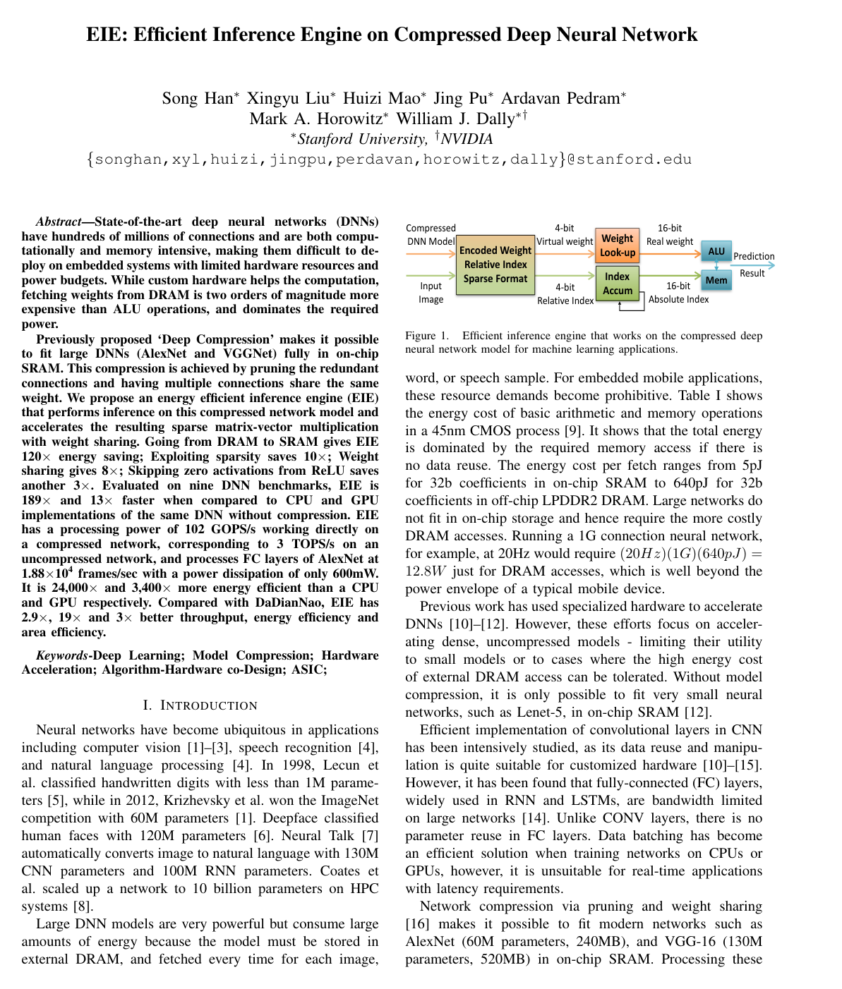
Previously proposed 'Deep Compression' makes it possible to fit large DNNs (AlexNet and VGGNet) fully in on-chip SRAM. This compression is achieved by pruning the redundant connections and having multiple connections share the same weight. We propose an energy efficient inference engine (EIE) that performs inference on this compressed network model and accelerates the resulting sparse matrix-vector multiplication with weight sharing. Going from DRAM to SRAM gives EIE 120x energy saving; Exploiting sparsity saves 10x; Weight sharing gives 8x; Skipping zero activations from ReLU saves another 3x. Evaluated on nine DNN benchmarks, EIE is 189x and 13x faster when compared to CPU and GPU implementations of the same DNN without compression. EIE has a processing power of 102GOPS/s working directly on a compressed network, corresponding to 3TOPS/s on an uncompressed network, and processes FC layers of AlexNet at 1.88x10^4 frames/sec with a power dissipation of only 600mW. It is 24,000x and 3,400x more energy efficient than a CPU and GPU respectively. Compared with DaDianNao, EIE has 2.9x, 19x and 3x better throughput, energy efficiency and area efficiency.

Table of Contents

  • I Introduction
  • II Motivation
  • III DNN Compression and Parallelization
  • III-A Computation
  • III-B Representation
  • III-C Parallelizing Compressed DNN
  • IV Hardware Implementation
  • V Evaluation Methodology
  • VI Experimental Results
  • VI-A Performance
  • VI-B Energy
  • VI-C Design Space Exploration
  • VII Discussion
  • VII-A Workload Partitioning
  • VII-B Scalability
  • VII-C Flexibility
  • VIII Comparison with Related Work
  • IX Conclusion
  • References

Knowls

  1. Knowl 1 — Compressed Matrix-Vector Computation with Dual Sparsity and Weight Sharing

    equation

    In a compressed fully-connected layer with weight pruning, weight sharing, and ReLU activations, the computation of the ii-th output activation bib_i from an input activation vector aa and a weight matrix WW is defined as:

    bi=ReLU(∑j∈Xi∩YS[Iij]aj)b_i = \text{ReLU}\left( \sum_{j \in X_i \cap Y} S[I_{ij}] a_j \right)

    where:

    • aja_j is the jj-th element of the input activation vector a∈RNa \in \mathbb{R}^N.
    • bib_i is the ii-th element of the output activation vector b∈RMb \in \mathbb{R}^M.
    • Xi={j∣Wij≠0}X_i = \{j \mid W_{ij} \neq 0\} is the set of column indices where the weights in row ii of the pruned sparse weight matrix WW are non-zero, representing static weight sparsity.
    • Y={j∣aj≠0}Y = \{j \mid a_j \neq 0\} is the set of column indices where the input activations are non-zero, representing dynamic activation sparsity (typically generated by ReLU non-linearities in previous layers).
    • Iij∈{0,1,…,15}I_{ij} \in \{0, 1, \dots, 15\} is a 4-bit integer index stored in the compressed matrix format representing the quantized weight at position (i,j)(i, j).
    • SS is a 16-entry shared weight table (codebook) storing 16-bit real weight values, such that S[Iij]S[I_{ij}] retrieves the shared weight corresponding to index IijI_{ij}.
    • ReLU(x)=max⁡(0,x)\text{ReLU}(x) = \max(0, x) is the rectified linear activation function.

    Computation and memory references are performed strictly for indices j∈Xi∩Yj \in X_i \cap Y, skipping operations whenever an input activation aj=0a_j = 0 or a weight Wij=0W_{ij} = 0.

  2. Knowl 2 — Interleaved CSC Storage Format and Row-Wise Workload Partitioning

    model/method

    To parallelize sparse matrix-vector multiplication (b=Wab = W a) across an array of NN processing elements (PEs) while exploiting both weight and activation sparsity:

    1. Row-Wise Distribution: Rows of the weight matrix WW, output activation elements bib_i, and input activation elements aia_i are interleaved across PEs such that PEk\text{PE}_k stores all elements with row/element index ii satisfying i≡k(modN)i \equiv k \pmod N. This keeps the accumulation of each output activation bib_i strictly local to PEk\text{PE}_k.

    2. Relative Indexed CSC Format: Within each PEk\text{PE}_k, its subset of column jj is stored in a modified Compressed Sparse Column (CSC) format consisting of three arrays:

      • vv: An array of 4-bit virtual weight codebook indices for non-zero weights in that PE's column slice.
      • zz: An array of 4-bit relative row indices, where each entry records the number of zero entries between consecutive non-zeros in the PE's local column slice. If more than 15 zeros appear between consecutive non-zeros, a padded entry (v=0,z=15)(v=0, z=15) is inserted.
      • pp: A 16-bit pointer array where pjp_j points to the start index of column jj in the vv and zz arrays, with the length of column jj's non-zero segment given by pj+1−pjp_{j+1} - p_j.
    3. Execution Pattern: Non-zero activations aja_j along with their column indices jj are broadcast sequentially to all PEs. Each PE looks up [pj,pj+1−1][p_j, p_{j+1}-1], fetches its local (v,z)(v, z) pairs, decodes the absolute row address by accumulating relative indices zz, and accumulates the products S[v]×ajS[v] \times a_j directly into its local destination registers without requiring inter-PE reductions.

  3. Knowl 3 — EIE Processing Element Microarchitecture and Pipeline

    model/method

    Each Processing Element (PE) in the Efficient Inference Engine (EIE) accelerates the compressed matrix-vector multiply using specialized functional units:

    1. Activation Queue: An 8-entry FIFO queue that buffers incoming broadcast (aj,j)(a_j, j) pairs to decouple activation broadcast from PE computation and absorb load imbalances across PEs.
    2. Pointer Read Unit: Contains two single-ported 16 KB SRAM banks (32 KB total pointer SRAM) holding 16-bit pointers. Using the least significant bit (LSB) of the column address to select between the even and odd banks allows fetching start pointer pjp_j and end pointer pj+1p_{j+1} in a single cycle.
    3. Sparse Matrix Read Unit: A 128 KB, 64-bit wide SRAM holding packed 8-bit (v,z)(v, z) entries (4-bit weight codebook index vv and 4-bit relative row index zz). It fetches 8 entries per 64-bit access, providing one entry per clock cycle over 8 cycles.
    4. Weight Decoder: A 16-entry lookup table mapping 4-bit codebook index vv to a 16-bit fixed-point weight S[v]S[v].
    5. Address Accumulator: A running accumulator that sums the 4-bit relative row index zz to compute the absolute row address xx of the destination activation.
    6. Arithmetic Unit: A 16-bit fixed-point multiply-accumulator performing bx←bx+S[v]×ajb_x \leftarrow b_x + S[v] \times a_j. It includes an accumulator bypass path to handle consecutive writes to the same destination row accumulator without pipeline stalls.
    7. Activation Read/Write Unit: Contains two ping-pong register files (each storing 64 16-bit activations, totaling 4K activations across a 64-PE array) backed by a 2 KB activation SRAM. The register files alternate source and destination roles across consecutive layers, eliminating inter-layer data transfer overhead.

    The PE executes a 4-stage pipeline for updating an activation:

    • Stage 1: Codebook lookup and address accumulation (in parallel).
    • Stage 2: Output activation read and input activation multiplication (in parallel).
    • Stage 3: Shift and add.
    • Stage 4: Output activation write.
  4. Knowl 4 — Distributed Leading Non-Zero Detection Hierarchy

    model/method

    To dynamically identify and broadcast non-zero input activations from the activation register files without sequential scanning overhead, EIE uses a distributed hierarchical quadtree network:

    1. Local Detection: Each group of 4 PEs performs local leading non-zero detection across its subset of the activation vector.
    2. Leading Non-Zero Detection (LNZD) Quadtree: The result is passed to an LNZD node. Each LNZD node selects the next non-zero activation among its four child inputs and routes the selected value and its index up the tree.
    3. Root / Central Control Unit (CCU): At the root of the quadtree, the CCU receives the global next non-zero activation aja_j and its index jj.
    4. H-Tree Broadcast: The CCU broadcasts (aj,j)(a_j, j) to all PEs via an H-tree distribution network. Because consuming a single column takes multiple PE execution cycles, the broadcast latency across the H-tree is completely decoupled from the critical path and hidden behind computation.

    For a 64-PE system, a total of 21 LNZD nodes are arranged across 3 hierarchical levels (16+4+1=2116 + 4 + 1 = 21). A single synthesized LNZD unit occupies 189 μm2189\,\mu\text{m}^2 and consumes 0.023 mW0.023\,\text{mW} in 45nm CMOS technology.

  5. Knowl 5 — Hardware Implementation and Power/Area Breakdown in 45nm CMOS

    data/table

    EIE was implemented in Verilog RTL, synthesized with Synopsys Design Compiler under TSMC 45nm GP standard VT library (worst-case PVT corner), and placed and routed using Synopsys IC Compiler. SRAM power and area were modeled using Cacti, with switching activity annotated from RTL simulation.

    The PE operates at a clock frequency of 800 MHz800\,\text{MHz} with a critical path delay of 1.15 ns1.15\,\text{ns}. A single PE occupies 0.638 mm20.638\,\text{mm}^2 (638,024 μm2638,024\,\mu\text{m}^2) and dissipates 9.157 mW9.157\,\text{mW} of power. A 64-PE array occupies 40.8 mm240.8\,\text{mm}^2 and dissipates 590 mW590\,\text{mW}, providing an effective processing throughput of 102 GOP/s102\,\text{GOP/s} directly on compressed models (equivalent to 3 TOP/s3\,\text{TOP/s} on dense uncompressed models given 10×10\times weight sparsity and 3×3\times activation sparsity).

    Component / Module Power [mW] (%) Area [μm2\mu\text{m}^2] (%)
    Total 9.157 (100.00%) 638,024 (100.00%)
    Breakdown by Component Type:
    Memory 5.416 (59.15%) 594,786 (93.22%)
    Clock network 1.874 (20.46%) 866 (0.14%)
    Register 1.026 (11.20%) 9,465 (1.48%)
    Combinational 0.841 (9.18%) 8,946 (1.40%)
    Filler cell - 23,961 (3.76%)
    Breakdown by Module:
    Activation queue 0.112 (1.23%) 758 (0.12%)
    Pointer Read Unit (PtrRead) 1.807 (19.73%) 121,849 (19.10%)
    Sparse Matrix Read Unit (SpmatRead) 4.955 (54.11%) 469,412 (73.57%)
    Arithmetic Unit (ArithmUnit) 1.162 (12.68%) 3,110 (0.49%)
    Activation Read/Write Unit (ActRW) 1.122 (12.25%) 18,934 (2.97%)
    Filler cell - 23,961 (3.76%)

    SRAM dominates the physical design of each PE, accounting for 93.22% of total area and 59.15% of total power.

  6. Knowl 6 — Platform Comparison on Deep Neural Network Fully-Connected Layers

    data/table

    Performance, power, area, and energy efficiency for matrix-vector multiplication on the FC7 layer of AlexNet (without batching, batch size = 1) across different computing platforms:

    Platform Core-i7 GeForce Tegra A-Eye DaDianNao TrueNorth EIE EIE
    5930K Titan X K1 (64PE) (28nm, 256PE)
    Year 2014 2015 2014 2015 2014 2014 2016 2016
    Platform Type CPU GPU mGPU FPGA ASIC ASIC ASIC ASIC
    Technology 22nm 28nm 28nm 28nm 28nm 28nm 45nm 28nm
    Clock (MHz) 3500 1075 852 150 606 Async 800 1200
    Memory type DRAM DRAM DRAM DRAM eDRAM SRAM SRAM SRAM
    Max Model Size <<16G <<3G <<500M <<500M 18M 256M 84M 336M
    Quantization 32b float 32b float 32b float 16b fixed 16b fixed 1b fixed 4b fixed 4b fixed
    Area (mm2\text{mm}^2) 356 601 - - 67.7 430 40.8 63.8
    Power (W) 73 159 5.1 9.63 15.97 0.18 0.59 2.36
    M×\timesV Throughput (frames/s) 162 4,115 173 33 147,938 1,989 81,967 426,230
    Area Efficiency (frames/s/mm2\text{mm}^2) 0.46 6.85 - - 2,185 4.63 2,009 6,681
    Energy Efficiency (frames/J) 2.22 25.9 33.9 3.43 9,263 10,839 138,927 180,606

    Across nine benchmark layers from AlexNet, VGG-16, and NeuralTalk (evaluated with batch size 1):

    • EIE (64 PEs, 45nm) achieves average speedups of 189×189\times, 13×13\times, and 307×307\times compared to CPU (Core i7-5930K), desktop GPU (Titan X), and mobile GPU (Tegra K1) executing uncompressed dense models.
    • EIE consumes 24,000×24,000\times, 3,400×3,400\times, and 2,700×2,700\times less energy compared to CPU, desktop GPU, and mobile GPU, respectively.
    • Compared to DaDianNao scaled to 28nm, EIE with 256 PEs demonstrates 2.9×2.9\times higher throughput, 3×3\times higher area efficiency, and 19×19\times higher energy efficiency.
  7. Knowl 7 — Theoretical and Empirical Factors of Energy Reduction in EIE

    theoretical result

    The energy reduction of EIE over uncompressed baseline execution in matrix-vector multiplication originates from four multiplicative factors:

    1. On-Chip SRAM vs. External DRAM Access (120×120\times): Model compression allows network weights to fit entirely into on-chip SRAM, eliminating external DRAM traffic. In a 45nm CMOS process, a 32-bit access to 32 KB on-chip SRAM consumes 5 pJ5\,\text{pJ}, compared to 640 pJ640\,\text{pJ} for a 32-bit fetch from off-chip LPDDR2 DRAM, providing a 128×128\times energy reduction per access (effective 120×120\times system-level reduction).
    2. Static Weight Sparsity (10×10\times): Weight pruning removes redundant connections, reducing the total number of non-zero weights by approximately 10×10\times (leaving ≈10%\approx 10\% non-zero density) and reducing weight fetch volume by 10×10\times.
    3. Weight Sharing / Quantization (8×8\times): Quantizing weights to 4-bit codebook indices instead of 32-bit floating-point values reduces storage and memory access energy by 8×8\times.
    4. Dynamic Activation Sparsity (3×3\times): Exploiting ReLU activation sparsity skips computation and weight fetches for the ≈70%\approx 70\% of input activations that are zero, saving 65.14%65.14\% of computation cycles (3×3\times reduction).

    Multiplying these components gives a theoretical energy savings factor of: 120×10×8×3=28,800×120 \times 10 \times 8 \times 3 = 28,800\times

    The actual measured energy savings relative to desktop GPU (3,400×3,400\times) and mobile GPU (2,700×2,700\times) are approximately 10×10\times lower than the theoretical maximum due to the 4-bit relative row indexing overhead, load imbalance idle cycles, and the process technology disparity (45nm for EIE versus 28nm for the baseline GPUs).

  8. Knowl 8 — Sparse Matrix SRAM Interface Width Optimization

    empirical result

    The choice of memory interface width for the sparse matrix SRAM (Spmat SRAM) presents an energy trade-off between read access energy and wasted reads:

    • Access Energy Trade-Off: Wider SRAM interfaces reduce total read operations but increase the energy dissipated per read cycle (modeled via Cacti in 45nm CMOS).
    • Over-fetch Waste: In a 64-PE configuration executing an activation vector of length 4K with 10% weight density, each PE's column slice contains on average 4000×0.1/64=6.44000 \times 0.1 / 64 = 6.4 non-zero elements. Fetching more elements than present in a column wastes energy if the next column corresponds to a zero input activation (which is skipped).
    • Optimal Width: Evaluating interface widths of 32-bit, 64-bit, 128-bit, 256-bit, and 512-bit on AlexNet showed that a 64-bit SRAM interface (which yields exactly eight 8-bit packed (v,z)(v, z) entries per read) achieves the global minimum in total SRAM access energy across all layers.
  9. Knowl 9 — Activation Queue Depth and Load Balancing Dynamics

    empirical result

    Because weight distribution across columns creates variance in the number of non-zero elements per PE slice, processing elements experience dynamic load imbalance:

    • Load Balance Efficiency Metric: Defined as: η=1−Bubble Cycles (due to starvation)Total Computation Cycles\eta = 1 - \frac{\text{Bubble Cycles (due to starvation)}}{\text{Total Computation Cycles}}
    • Queue Depth Scaling: Varying the activation FIFO queue depth from 1 to 256 across nine benchmarks on a 64-PE system reveals that at a FIFO depth of 1, approximately 50% of ALU cycles are idle bubbles. Increasing queue depth smooths out work starvation, with load balancing efficiency improving sharply up to a depth of 8.
    • Diminishing Returns: Marginal efficiency gains plateau beyond a depth of 8 across all benchmarks, making depth 8 the optimal hardware configuration.
    • Matrix Dimension Impact: Small layers (such as NeuralTalk Word Embedding NT-We, with matrix dimensions 4096×6004096 \times 600 and 11%11\% sparsity) assign an average of only ≈1\approx 1 non-zero entry per column to each of 64 PEs, resulting in higher execution variance and lower load balance efficiency unless executed on 32 or fewer PEs.
  10. Knowl 10 — Fixed-Point Arithmetic Precision and Accuracy Impact

    empirical result

    EIE evaluates the trade-off between ALU precision, multiplier energy dissipation in 45nm CMOS, and ImageNet top-1 classification accuracy on AlexNet:

    • 32-bit Floating-Point: 80.3% accuracy, consuming 3.7 pJ3.7\,\text{pJ} per multiplication.
    • 32-bit Fixed-Point: Consumes 3.1 pJ3.1\,\text{pJ} per multiplication.
    • 16-bit Fixed-Point: 79.8% accuracy (a degradation of <0.5%< 0.5\%) while consuming 5×5\times less energy than 32-bit fixed-point and 6.2×6.2\times less energy than 32-bit floating-point.
    • 8-bit Fixed-Point: Accuracy drops precipitously to 53.0%, making it intolerable for inference.

    EIE adopts 16-bit fixed-point arithmetic for weight codebook values, multipliers, and accumulators. Because SRAM accounts for 93.22% of PE area and 59.15% of PE power, switching from 16-bit to 32-bit arithmetic would only affect the 16-entry codebook, ALU, and activation registers (with the 4-bit index in SRAM remaining unchanged), fitting easily within existing layout filler cell area (3.76% of PE area) without substantially impacting overall chip power or area.

  11. Knowl 11 — Scalability and Padding Zero Overhead with Processing Element Count

    empirical result

    EIE scales from 1 PE up to 256 PEs with near-linear performance gains across benchmark networks:

    • Interconnection Overhead: Inter-PE broadcast wire delay grows with O(NPE)O(\sqrt{N_{\text{PE}}}), but because each broadcast activation initiates a multi-cycle column computation within each PE, activation broadcast is completely pipelined and removed from the critical path.
    • Padding Zero Reduction: Padding zeros occur when the gap between consecutive non-zero weights along a column exceeds 15 (the maximum representable jump in a 4-bit relative index). Distributing matrix rows over a larger number of PEs reduces the absolute number of rows per PE, shortening the distance between non-zero elements and monotonically decreasing padding zero overhead as the PE count increases from 1 to 256.
    • Load Balance vs. Padding Trade-off: While increasing PE count slightly worsens load balance across PEs, the concurrent decrease in padding zeros reduces wasted computation cycles, maintaining near-constant compute efficiency across varying PE array sizes.

Coverage note — None was omitted. All major contributions, quantitative benchmarks, design trade-offs (SRAM width, FIFO depth, precision, scalability), and hardware architectural details have been captured.

References

  1. 1.A. Krizhevsky, I. Sutskever, and G. E. Hinton, “Imagenet classification with deep convolutional neural networks,” in NIPS, 2012.
  2. 2.C. Szegedy, W. Liu, Y. Jia, P. Sermanet, S. Reed, D. Anguelov, D. Erhan, V. Vanhoucke, and A. Rabinovich, “Going deeper with convolutions,” arXiv:1409.4842, 2014.
  3. 3.K. Simonyan and A. Zisserman, “Very deep convolutional networks for large-scale image recognition,” arXiv:1409.1556, 2014.
  4. 4.T. Mikolov, M. Karafiat, L. Burget, J. Cernock ý, and S. Khudanpur, “Recurrent neural network based language model.” in INTERSPEECH, September 26-30, 2010, 2010, pp. 1045–1048.
  5. 5.Y. LeCun, L. Bottou, Y. Bengio, and P. Haffner, “Gradient-based learning applied to document recognition,” Proceedings of the IEEE, vol. 86, no. 11, pp. 2278–2324, 1998.
  6. 6.Y. Taigman, M. Yang, M. Ranzato, and L. Wolf, “Deepface: Closing the gap to human-level performance in face verification,” in CVPR. IEEE, 2014, pp. 1701–1708.
  7. 7.A. Karpathy and L. Fei-Fei, “Deep visual-semantic alignments for generating image descriptions,” arXiv:1412.2306, 2014.
  8. 8.A. Coates, B. Huval, T. Wang, D. Wu, B. Catanzaro, and N. Andrew, “Deep learning with cots hpc systems,” in 30th ICML, 2013.
  9. 9.M. Horowitz. Energy table for 45nm process, Stanford VLSI wiki. [Online]. Available: https://sites.google.com/site/seecproject
  10. 10.T. Chen, Z. Du, N. Sun, J. Wang, C. Wu, Y. Chen, and O. Temam, “Diannao: a small-footprint high-throughput accelerator for ubiquitous machine-learning,” in ASPLOS, 2014.
  11. 11.Y. Chen, T. Luo, S. Liu, S. Zhang, L. He, J. Wang, L. Li, T. Chen, Z. Xu, N. Sun, and O. Temam, “Dadiannao: A machine-learning supercomputer,” in MICRO, December 2014.
  12. 12.Z. Du, R. Fasthuber, T. Chen, P. Ienne, L. Li, T. Luo, X. Feng, Y. Chen, and O. Temam, “Shidiannao: shifting vision processing closer to the sensor,” in ISCA. ACM, 2015, pp. 92–104.
  13. 13.C. Farabet, C. Poulet, J. Y. Han, and Y. LeCun, “Cnp: An fpga-based processor for convolutional networks,” in FPL, 2009.
  14. 14.J. Qiu, J. Wang, S. Yao, K. Guo, B. Li, E. Zhou, J. Yu, T. Tang, N. Xu, S. Song, Y. Wang, and H. Yang, “Going deeper with embedded fpga platform for convolutional neural network,” in FPGA, 2016.
  15. 15.A. Shafiee and et al., “ISAAC: A convolutional neural network accelerator with in-situ analog arithmetic in crossbars,” ISCA, 2016.
  16. 16.S. Han, J. Pool, J. Tran, and W. J. Dally, “Learning both weights and connections for efficient neural networks,” in Proceedings of Advances in Neural Information Processing Systems, 2015.
  17. 17.R. Girshick, “Fast R-CNN,” arXiv:1504.08083, 2015.
  18. 18.S. Hochreiter and J. Schmidhuber, “Long short-term memory,” Neural computation, 1997.
  19. 19.A. Graves and J. Schmidhuber, “Framewise phoneme classification with bidirectional lstm and other neural network architectures,” Neural Networks, 2005.
  20. 20.N. D. Lane and P. Georgiev, “Can deep learning revolutionize mobile sensing?” in International Workshop on Mobile Computing Systems and Applications. ACM, 2015, pp. 117–122.
  21. 21.Richard Dorrance and Fengbo Ren and Dejan Markovic, “A Scalable Sparse Matrix-vector Multiplication Kernel for Energy-efficient Sparse-blas on FPGAs,” in FPGA, 2014.
  22. 22.V. Nair and G. E. Hinton, “Rectified linear units improve restricted boltzmann machines,” in ICML, 2010.
  23. 23.S. Han, H. Mao, and W. J. Dally, “Deep compression: Compressing deep neural networks with pruning, trained quantization and huffman coding,” International Conference on Learning Representations 2016.
  24. 24.R. W. Vuduc, “Automatic performance tuning of sparse matrix kernels,” Ph.D. dissertation, UC Berkeley, 2003.
  25. 25.N. Muralimanohar, R. Balasubramonian, and N. P. Jouppi, “Cacti 6.0: A tool to model large caches,” HP Laboratories, pp. 22–31, 2009.
  26. 26.NVIDIA. Technical brief: NVIDIA jetson TK1 development kit bringing GPU-accelerated computing to embedded systems.
  27. 27.NVIDIA. Whitepaper: GPU-based deep learning inference: A performance and power analysis.
  28. 28.Y. Jia, E. Shelhamer, J. Donahue, S. Karayev, J. Long, R. Girshick, S. Guadarrama, and T. Darrell, “Caffe: Convolutional architecture for fast feature embedding,” arXiv:1408.5093, 2014.
  29. 29.J. Deng, W. Dong, R. Socher, L.-J. Li, K. Li, and L. Fei-Fei, “Imagenet: A large-scale hierarchical image database,” in Computer Vision and Pattern Recognition. 2009.
  30. 30.F. N. Iandola, S. Han, M. W. Moskewicz, K. Ashraf, W. J. Dally, and K. Keutzer, “Squeezenet: Alexnet-level accuracy with 50x fewer parameters and¡ 0.5mb model size,” arXiv:1602.07360, 2016.
  31. 31.Ling Zhuo and Viktor K. Prasanna, “Sparse Matrix-Vector Multiplication on FPGAs,” in FPGA, 2005.
  32. 32.V. Eijkhout, LAPACK working note 50: Distributed sparse data structures for linear algebra operations, 1992.
  33. 33.A. Lavin, “Fast algorithms for convolutional neural networks,” arXiv:1509.09308, 2015.
  34. 34.S. J. Hanson and L. Y. Pratt, “Comparing biases for minimal network construction with back-propagation,” in NIPS, 1989.
  35. 35.Y. LeCun, J. S. Denker, S. A. Solla, R. E. Howard, and L. D. Jackel, “Optimal brain damage.” in NIPs, vol. 89, 1989.
  36. 36.B. Hassibi, D. G. Stork et al., “Second order derivatives for network pruning: Optimal brain surgeon,” Advances in neural information processing systems, pp. 164–164, 1993.
  37. 37.E. L. Denton, W. Zaremba, J. Bruna, Y. LeCun, and R. Fergus, “Exploiting linear structure within convolutional networks for efficient evaluation,” in NIPS 2014.
  38. 38.X. Zhang, J. Zou, X. Ming, K. He, and J. Sun, “Efficient and accurate approximations of nonlinear convolutional networks,” arXiv:1411.4229, 2014.
  39. 39.B. Reagen, P. Whatmough, R. Adolf, S. Rama, H. Lee, S. K. Lee, J. M. Hernndez-Lobato, G.-Y. Wei, and D. Brooks, “Minerva: Enabling low-power, highly-accurate deep neural network accelerators,” ISCA, 2016.
  40. 40.S. K. Esser and et al., “Convolutional networks for fast, energyefficient neuromorphic computing,” arXiv:1603.08270, 2016.
  41. 41.C. Zhang, P. Li, G. Sun, Y. Guan, B. Xiao, and J. Cong, “Optimizing fpga-based accelerator design for deep convolutional neural networks,” in FPGA, 2015.
  42. 42.Alexander Monakov and Anton Lokhmotov and Arutyun Avetisyan, “Automatically tuning sparse matrix-vector multiplication for GPU architectures,” in HiPEAC, 2010.
  43. 43.N. Bell and M. Garland, “Efficient sparse matrix-vector multiplication on cuda,” Nvidia Technical Report NVR-2008-004, Tech. Rep., 2008.
  44. 44.Bell, Nathan and Garland, Michael, “Implementing Sparse Matrixvector Multiplication on Throughput-oriented Processors,” in High Performance Computing Networking, Storage and Analysis, 2009.
  45. 45.J. Fowers and K. Ovtcharov and K. Strauss and E.S. Chung and G. Stitt, “A high memory bandwidth fpga accelerator for sparse matrixvector multiplication,” in FCCM, 2014.

Citation

MLA
Han, S., et al. “EIE”. ACM SIGARCH Computer Architecture News, vol. 44, no. 3, 2016, pp. 243–54, https://doi.org/10.1145/3007787.3001163.
APA
Han, S., Liu, X., Mao, H., Pu, J., Pedram, A., Horowitz, M. A., & Dally, W. J. (2016). EIE. ACM SIGARCH Computer Architecture News, 44(3), 243–254. https://doi.org/10.1145/3007787.3001163
Chicago
Han, S., X. Liu, H. Mao, et al. 2016. “EIE”. ACM SIGARCH Computer Architecture News 44 (3): 243–54. https://doi.org/10.1145/3007787.3001163.
Harvard
Han, S. et al. (2016) “EIE”, ACM SIGARCH Computer Architecture News, 44(3), pp. 243–254. Available at: https://doi.org/10.1145/3007787.3001163.
Vancouver
1. Han S, Liu X, Mao H, Pu J, Pedram A, Horowitz MA, Dally WJ (2016) EIE. ACM SIGARCH Computer Architecture News 44:243–254

BibTeX

@article{Han_2016, title={EIE: efficient inference engine on compressed deep neural network}, volume={44}, ISSN={0163-5964}, url={http://dx.doi.org/10.1145/3007787.3001163}, DOI={10.1145/3007787.3001163}, number={3}, journal={ACM SIGARCH Computer Architecture News}, publisher={Association for Computing Machinery (ACM)}, author={Han, Song and Liu, Xingyu and Mao, Huizi and Pu, Jing and Pedram, Ardavan and Horowitz, Mark A. and Dally, William J.}, year={2016}, month=June, pages={243–254} }
Metadata:Crossref

Access the Paper

This paper is available from its original source. Click below to access the PDF.

Open PDF