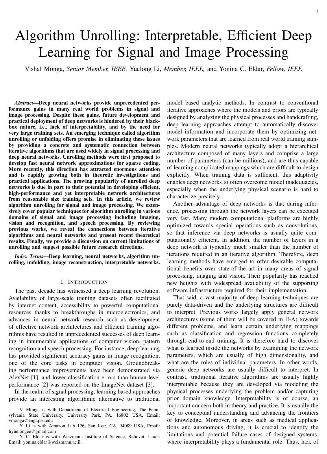
Algorithm Unrolling: Interpretable, Efficient Deep Learning for Signal and Image Processing

Vishal MongaYuelong LiYonina C. Eldar

article2019IEEE Signal Processing Magazine1,438 citationsIEEE Signal Processing Magazine Best Paper Award (2024)

Systematizes algorithm unrolling methods that transform classical iterative signal processing algorithms into interpretable, sample-efficient deep neural networks, detailing theoretical foundations and practical applications across imaging, computer vision, and speech processing.

Listen

Modern deep neural networks deliver state-of-the-art performance across computer vision and signal processing, yet their practical deployment is severely limited by their black-box nature and excessive data hunger. Standard generic networks contain millions of unconstrained parameters, making them difficult to interpret, prone to severe overfitting when data is scarce, and challenging to certify for mission-critical settings such as medical diagnosis or autonomous systems. Conversely, classical model-based iterative algorithms are highly transparent and incorporate explicit physics and domain knowledge, but they are often computationally slow and struggle when physical models are imperfect.

The article evaluates algorithm unrolling—also known as algorithm unfolding—as a principled framework that bridges classical iterative algorithms and deep learning. Its main objective is to demonstrate how unrolling creates deep architectures that are inherently interpretable, computationally efficient, and robust under limited training data across diverse signal and image processing domains.

The authors conducted a comprehensive synthesis of foundational concepts, mathematical methodologies, theoretical convergence analyses, and cross-domain empirical implementations. The approach conceptually maps each iteration of a classical model-based algorithm into a single layer of a neural network and sets the algorithm's operational parameters (such as filter coefficients, dictionary matrices, and regularization weights) as learnable network parameters optimized through end-to-end back-propagation on real-world datasets.

Key findings show that algorithm unrolling consistently outperforms both traditional iterative algorithms and generic deep networks. First, unrolled networks achieve massive computational speedups during inference compared to iterative baselines, running roughly 4 to over 1,000 times faster—such as Learned ISTA operating 20 times faster than standard ISTA and DUBLID executing blind deblurring 1,000 times faster than total-variation baselines. Second, unrolling reduces parameter dimensionality by several orders of magnitude compared to generic networks; for example, DUBLID requires more than 100 times fewer parameters than leading deep restoration networks while achieving superior image quality. Third, unrolled models generalize substantially better in low-data regimes—in magnetic resonance imaging, the unrolled ADMM-CSNet achieved target accuracy using 10% less sampled data while outperforming standard deep networks by approximately 3 dB peak signal-to-noise ratio. Finally, recent theoretical analyses confirm that unrolled sparse coding models can achieve linear convergence rates, proving that their empirical acceleration is backed by rigorous mathematical foundations.

These results provide direct operational benefits for technology deployment and risk management. By explicitly embedding physical models into network layers, unrolled models preserve architectural transparency, reducing the risks and safety concerns of deploying black-box algorithms in sensitive domains like clinical imaging. Furthermore, the extreme reduction in memory footprint and compute latency lowers computational hardware costs and enables high-performance edge deployment on resource-constrained platforms, such as mobile devices, embedded cameras, and real-time power grid monitors.

Organizations developing machine learning for scientific and physical systems should adopt algorithm unrolling as a primary architectural paradigm, especially when training data is constrained or model interpretability is mandatory. When implementing unrolling, teams face a trade-off: tying parameters across layers yields maximum parameter efficiency but risks training instability similar to recurrent networks, whereas using layer-specific parameters expands empirical capacity at the cost of strict mathematical convergence guarantees. Practitioners should utilize greedy layer-wise pre-training to stabilize optimization and carefully select base iterative algorithms whose operators are smooth or can be approximated smoothly.

While empirical results across medical imaging, speech processing, and remote sensing are robust, several limitations and uncertainties remain. Deep theoretical explanations for why unrolling works effectively in complex visual recognition tasks remain incomplete. Furthermore, standardized initialization schemes and architectural techniques (such as batch normalization equivalents) tailored specifically for custom unrolled structures are still evolving. Readers should proceed with measured caution regarding training stability until end-to-end training protocols are validated for specific operational pipelines.

Amazon Pennsylvania State University Weizmann Institute of Science image denoising interpretability network architecture algorithm unrolling deep unfolding interpretable neural networks

arXiv: 1912.10557

Paper: Fundamentals of Recurrent Neural Network (RNN) and Long Short-Term Memory (LSTM) Network, Alex Sherstinsky (2018). It provides the mathematical first-principles derivation and theoretical justification for unrolling iterative recurrence into feedforward networks, which directly underpins algorithm unrolling.
Paper: Deep Image Prior, Dmitry Ulyanov et al. (2017). It illustrates how deep neural architectures encode structural priors for inverse problems in imaging, establishing a foundational perspective for connecting iterative signal processing solvers to neural networks.
Paper: Deep Residual Learning for Image Recognition, Kaiming He et al. (2016). It introduces deep residual learning, providing the fundamental skip-connection architecture that iterative algorithm unfolding emulates when mapping algorithmic step updates to neural layers.
Paper: Training Deep Nets with Sublinear Memory Cost, Tianqi Chen et al. (2016). It establishes computational graph optimization and memory-efficient backpropagation through time for unrolled networks, which is crucial for training unrolled iterative algorithms.
Paper: Methods for interpreting and understanding deep neural networks, Grégoire Montavon et al. (2018). It surveys foundational interpretability and explainability methods for deep neural networks, providing the context for why unrolling is sought as an interpretable architectural alternative.

Paper: Learning nonlinear operators via DeepONet based on the universal approximation theorem of operators, Lu Lu et al. (2021). It extends the paradigm of learning mathematical operators from unrolled iterative signal solvers to general continuous nonlinear operators through operator learning networks.
Paper: Pruning neural networks without any data by iteratively conserving synaptic flow, Hidenori Tanaka et al. (2020). It advances network efficiency and sparsity theory by showing how structured subnetworks can be identified at initialization, offering complementary optimization strategies for structured, unrolled deep models.
Paper: Designing Network Design Spaces, Ilija Radosavovic et al. (2020). It explores systematic design spaces for deep neural network architectures, providing a methodology to scale and structure model design beyond manual algorithmic unrolling.
Paper: KAN: Kolmogorov-Arnold Networks, Ziming Liu et al. (2025). It introduces Kolmogorov-Arnold Networks as an alternative interpretable mathematical architecture for scientific computing, building on the broader goal of interpretable neural modeling discussed in algorithm unrolling.

Cover for Algorithm Unrolling: Interpretable, Efficient Deep Learning for Signal and Image Processing

Abstract

Deep neural networks provide unprecedented performance gains in many real world problems in signal and image processing. Despite these gains, future development and practical deployment of deep networks is hindered by their blackbox nature, i.e., lack of interpretability, and by the need for very large training sets. An emerging technique called algorithm unrolling or unfolding offers promise in eliminating these issues by providing a concrete and systematic connection between iterative algorithms that are used widely in signal processing and deep neural networks. Unrolling methods were first proposed to develop fast neural network approximations for sparse coding. More recently, this direction has attracted enormous attention and is rapidly growing both in theoretic investigations and practical applications. The growing popularity of unrolled deep networks is due in part to their potential in developing efficient, high-performance and yet interpretable network architectures from reasonable size training sets. In this article, we review algorithm unrolling for signal and image processing. We extensively cover popular techniques for algorithm unrolling in various domains of signal and image processing including imaging, vision and recognition, and speech processing. By reviewing previous works, we reveal the connections between iterative algorithms and neural networks and present recent theoretical results. Finally, we provide a discussion on current limitations of unrolling and suggest possible future research directions.

Topics

image denoising interpretability network architecture speech processing theoretical result training sample coding mode convolutional neural networks recurrent neural networks adaptive algorithms

Keywords

algorithm unrolling deep unfolding interpretable neural networks computational imaging sparse representation blind image denoising signal processing

I Introduction
II Generating Interpretable Networks through Algorithm Unrolling
II-A Conventional Neural Networks
II-B Unrolling Sparse Coding Algorithms into Deep Networks
II-C Algorithm Unrolling in General
III Unrolling in Signal and Image Processing Problems
III-A Applications in Computational Imaging
III-B Applications in Medical Imaging
III-C Applications in Vision and Recognition
III-D Other Signal Processing Applications
III-E Enhancing Efficiency Through Unrolling
IV Conceptual Connections and Theoretical Analysis
IV-A Connections to Sparse Coding
IV-B Connections to Kalman Filtering
IV-C Connections to Differential Equations and Variational Methods
IV-D Connections to Statistical Inference and Sampling
IV-E Selected Theoretical Studies
V Perspectives and Recent Trends
V-A Distilling the Power of Algorithm Unrolling
V-B Trends: Expanding Application Landscape and Addressing Implementation Concerns
V-C Alternative Approaches
VI Conclusions
References

Knowls

Knowl 1 — Algorithm Unrolling Framework for Deep Neural Network Construction
model/method
Algorithm unrolling (or unfolding) maps an iterative optimization algorithm into a deep neural network architecture. Consider an iterative algorithm whose state $z \in \mathbb{R}^d$ updates according to an iteration step function $h$ parameterized by a vector $\theta$ :

$z^{l+1} = h(z^l; \theta^l), \quad l = 0, 1, \dots, L-1$

An unrolled deep network is constructed by cascading $L$ such iteration steps as successive network layers. Passing an initial input $z^0$ through the $L$ -layer network corresponds to executing $L$ iterations (finite truncation) of the algorithm.

The algorithm parameters $\theta^l$ (such as step sizes, regularization parameters, transform matrices, or filter coefficients) become trainable network parameters. Rather than setting these parameters analytically or via manual cross-validation, they are optimized end-to-end across a dataset of training pairs $(y_n, x_n^*)_{n=1}^N$ using backpropagation and gradient descent on a loss function $\ell(\hat{z}^L(y_n; \{\theta^l\}), x_n^*)$ .

The resulting network inherits domain-specific structure and interpretability from the underlying physical/algorithmic formulation while achieving higher computational speed (by executing fewer truncated iterations) and improved parameter adaptivity compared to handcrafted algorithms.
Knowl 2 — Learned Iterative Shrinkage and Thresholding Algorithm (LISTA)
model/method
Learned Iterative Shrinkage and Thresholding Algorithm (LISTA) unrolls the Iterative Shrinkage and Thresholding Algorithm (ISTA) used for solving the sparse coding problem:

$\min_{x \in \mathbb{R}^m} \frac{1}{2} \|y - Wx\|_2^2 + \lambda \|x\|_1$

where $y \in \mathbb{R}^n$ is the observed measurement, $W \in \mathbb{R}^{n \times m}$ with $m > n$ is an over-complete dictionary, and $\lambda > 0$ is a sparsity penalty. Standard ISTA updates the sparse code estimate via:

$x^{l+1} = \mathcal{S}_\lambda \left( \left( I - \frac{1}{\mu} W^T W \right) x^l + \frac{1}{\mu} W^T y \right)$

where $\mu > 0$ is a step-size parameter, and $\mathcal{S}_\lambda(\cdot)$ is the elementwise soft-thresholding operator defined as:

$\mathcal{S}_\lambda(u) = \text{sign}(u) \cdot \max\{|u| - \lambda, 0\}$

LISTA unrolls $L$ iterations of ISTA into an $L$ -layer feedforward network with learnable parameter matrices and thresholds at each layer $l$ :

$x^{l+1} = \mathcal{S}_{\lambda^l} \left( W_t^l x^l + W_e^l y \right), \quad l = 0, \dots, L-1$

where $W_t^l \in \mathbb{R}^{m \times m}$ , $W_e^l \in \mathbb{R}^{m \times n}$ , and threshold $\lambda^l > 0$ are learnable weights. Given training pairs of measurements and ground-truth sparse codes $(y_n, x^*_n)_{n=1}^N$ , the network is trained end-to-end by minimizing the mean squared error loss:

$\mathcal{L}(\{W_t^l, W_e^l, \lambda^l\}_{l=0}^{L-1}) = \frac{1}{N} \sum_{n=1}^N \|\hat{x}_n(y_n) - x_n^*\|_2^2$

Trained LISTA networks achieve convergence in an order of magnitude fewer layers than the number of iterations required by conventional ISTA.
Knowl 3 — Asymptotic Weight Coupling and Convergence Guarantees for LISTA
theoretical result
For an unrolled sparse coding network with observation model $y = W x^* + e$ where $x^* \in \mathbb{R}^m$ is an $s$ -sparse vector ( $\|x^*\|_0 \le s$ ), unrolling the Iterative Hard Thresholding (IHT) or ISTA algorithm reveals structural constraints on optimal network weights:
1. In an unrolled IHT network $x^{l+1} = \mathcal{H}_k(W_t^l x^l + W_e^l y)$ , where $\mathcal{H}_k$ retains the $k$ largest elements in magnitude, exact recovery of $x^*$ requires that the weight matrices satisfy: $W_t^l = I - \Gamma^l W$ for some matrix $\Gamma^l \in \mathbb{R}^{m \times n}$ .
2. For layer-specific LISTA networks $x^{l+1} = \mathcal{S}_{\lambda^l}(W_t^l x^l + W_e^l y)$ , under mild regularity conditions, whenever the network successfully recovers $x^*$ , the parameters asymptotically satisfy the weight coupling condition:
$W_t^l - (I - W_e^l W) \to 0 \quad \text{as } l \to \infty$
1. Constraining the network parameterization to the coupled form $W_t^l = I - W_e^l W$ together with a support selection mechanism (LISTA-CPSS) guarantees a linear convergence rate to the true sparse code $x^*$ .
2. In Analytic LISTA (ALISTA), the weights $W_e^l$ can be computed analytically by minimizing mutual column incoherence with dictionary $W$ rather than being learned via backpropagation, reducing parameter dimensionality while preserving linear convergence.
Knowl 4 — Deep Unrolling for Blind Deblurring (DUBLID)
model/method
Deep Unrolling for Blind Deblurring (DUBLID) unrolls the Half-Quadratic Splitting algorithm for blind image deblurring under an unknown blur kernel $k$ and latent sharp image $x$ governed by $y = k * x + n$ .

The formulation optimizes filtered domain gradients across $C$ learnable filters $\{f_i\}_{i=1}^C$ :

$\min_{k, \{g_i, z_i\}_{i=1}^C} \sum_{i=1}^C \left( \frac{1}{2}\|f_i * y - k * g_i\|_2^2 + \lambda_i \|z_i\|_1 + \frac{1}{2\zeta_i}\|g_i - z_i\|_2^2 \right) + \frac{\epsilon}{2}\|k\|_2^2 \quad \text{s.t.} \quad \|k\|_1 = 1, k \ge 0$

where $\{z_i\}_{i=1}^C$ are auxiliary splitting variables, and $\lambda_i, \zeta_i, \epsilon > 0$ are regularization parameters.

DUBLID unrolls $L$ iterations of analytic alternating updates in the Discrete Fourier Transform (DFT) domain $\mathcal{F}(\cdot)$ :

$g_i^{l+1} = \mathcal{F}^{-1} \left( \frac{\zeta_i^l (\hat{k}^l)^* \odot (\hat{f}_i^l \odot \hat{y}) + \hat{z}_i^l}{\zeta_i^l |\hat{k}^l|^2 + 1} \right)$

$z_i^{l+1} = \mathcal{S}_{\lambda_i^l \zeta_i^l}\left(g_i^{l+1}\right)$

$k^{l+1} = \mathcal{N}_1 \left( \left[ \mathcal{F}^{-1} \left( \frac{\sum_{i=1}^C (\hat{z}_i^{l+1})^* \odot (\hat{f}_i^l \odot \hat{y})}{\sum_{i=1}^C |\hat{z}_i^{l+1}|^2 + \epsilon} \right) \right]_+ \right)$

where $\hat{u} = \mathcal{F}(u)$ , $(\cdot)^*$ denotes complex conjugate, $\odot$ is elementwise multiplication, $\mathcal{S}_{\beta}$ is soft-thresholding, $[\cdot]_+$ is ReLU, and $\mathcal{N}_1(\cdot)$ normalizes the sum to 1.

After $L$ layers, the latent sharp image is retrieved in a final layer by linear least-squares:

$\hat{x} = \mathcal{F}^{-1} \left( \frac{(\hat{k}^L)^* \odot \hat{y} + \sum_{i=1}^C \eta_i (\hat{f}_i^L)^* \odot \hat{g}_i^L}{|\hat{k}^L|^2 + \sum_{i=1}^C \eta_i |\hat{f}_i^L|^2} \right)$

Filter weights $\{f_i^l\}$ and parameters $\{\lambda_i^l, \zeta_i^l, \eta_i\}$ are trained end-to-end via backpropagation using a translation-invariant MSE loss.
Knowl 5 — ADMM-CSNet for Compressive Sensing Reconstruction
model/method
ADMM-CSNet unrolls the Alternating Direction Method of Multipliers (ADMM) algorithm to reconstruct a signal $x \in \mathbb{R}^n$ from underdetermined linear compressive sensing measurements $y = \Phi x \in \mathbb{C}^m$ ( $m < n$ ). The generalized CS minimization problem is:

$\min_x \frac{1}{2} \|\Phi x - y\|_2^2 + \sum_{i=1}^C \lambda_i g(D_i x)$

where $\{D_i\}_{i=1}^C$ are transform operators, $g(\cdot)$ is a sparsity-inducing regularizer, and $\lambda_i > 0$ are regularization weights. Variable splitting $z_i = D_i x$ and introduction of multipliers $\alpha_i$ yield the augmented Lagrangian:

$\mathcal{L}_\rho(x, \{z_i\}, \{\alpha_i\}) = \frac{1}{2}\|\Phi x - y\|_2^2 + \sum_{i=1}^C \left[ \lambda_i g(z_i) + \frac{\rho_i}{2}\|D_i x - z_i + \alpha_i\|_2^2 \right]$

Each layer $l$ of ADMM-CSNet implements the three-step alternating minimization:

$x^l = \left( \Phi^H \Phi + \sum_{i=1}^C \rho_i D_i^T D_i \right)^{-1} \left( \Phi^H y + \sum_{i=1}^C \rho_i D_i^T (z_i^{l-1} - \alpha_i^{l-1}) \right)$

$z_i^l = \mathcal{P}_g \left( D_i x^l + \alpha_i^{l-1}; \frac{\lambda_i}{\rho_i} \right), \quad \forall i=1, \dots, C$

$\alpha_i^l = \alpha_i^{l-1} + \eta_i (D_i x^l - z_i^l), \quad \forall i=1, \dots, C$

where $\mathcal{P}_g(u; \gamma)$ is the proximal operator associated with $g$ . The operators $D_i$ (represented as convolution kernels), regularization weights $\lambda_i$ , penalty parameters $\rho_i$ , and multiplier step sizes $\eta_i$ are learned per layer by training end-to-end via normalized Root-Mean-Square Error.
Knowl 6 — Convolutional Robust PCA (CORONA) for Clutter Suppression
model/method
Convolutional Robust Principal Component Analysis (CORONA) unrolls matrix ISTA for low-rank and sparse matrix decomposition to separate tissue clutter from blood flow signals in medical ultrasound imaging.

Given an acquired data matrix $D = H_1 L + H_2 S + N \in \mathbb{C}^{m \times n}$ , where $L$ is low-rank tissue clutter, $S$ is row-sparse blood echoes, $H_1, H_2$ are measurement matrices, and $N$ is noise, the decomposition problem is:

$\min_{L, S} \frac{1}{2} \|D - (H_1 L + H_2 S)\|_F^2 + \lambda_1 \|L\|_* + \lambda_2 \|S\|_{1,2}$

where $\|\cdot\|_*$ is the nuclear norm and $\|\cdot\|_{1,2}$ is the mixed $\ell_{1,2}$ norm. CORONA converts matrix multiplications into 2D convolutions $P_i^l * (\cdot)$ , yielding layer updates:

$L^{l+1} = \mathcal{T}_{\lambda_1^l} \left( P_5^l * L^l + P_3^l * S^l + P_1^l * D \right)$

$S^{l+1} = \mathcal{S}_{\lambda_2^l}^{1,2} \left( P_6^l * S^l + P_4^l * L^l + P_2^l * D \right)$

where $\mathcal{T}_\lambda(X)$ applies soft-thresholding to the singular values of matrix $X$ , and $\mathcal{S}_\lambda^{1,2}(X)$ applies row-wise soft-thresholding. The convolution filter banks $\{P_1^l, \dots, P_6^l\}$ and layer thresholds $\{\lambda_1^l, \lambda_2^l\}$ are learned end-to-end, producing a CNN-like structure that outperforms generic deep architectures while using an order of magnitude fewer parameters.
Knowl 7 — Unrolling Conditional Random Fields into Recurrent Neural Networks (CRF-RNN)
model/method
CRF-RNN reformulates Mean-Field (MF) approximate inference in fully-connected Conditional Random Fields (CRFs) as a recurrent neural network for end-to-end semantic segmentation. Given image pixel nodes $\mathcal{V}$ , edges $\mathcal{E}$ , and label set $\mathcal{L}$ , the CRF energy is:

$E(\{l_p\}_{p \in \mathcal{V}}) = \sum_{p \in \mathcal{V}} \phi_p(l_p) + \sum_{(p,q) \in \mathcal{E}} \psi_{p,q}(l_p, l_q)$

where unary potentials $\phi_p(l_p)$ are computed by a front-end Fully Convolutional Network (FCN), and pairwise potentials are Gaussian mixtures $\psi(l_p, l_q) = \mu(l_p, l_q) \sum_{m=1}^M w^m G^m(f_p, f_q)$ over pixel feature vectors $f_p, f_q$ .

Each iteration of the Mean-Field inference is unrolled into dedicated differentiable neural network layers:
1. Message Passing: $\tilde{Q}_p^m(l) \leftarrow \sum_{q \neq p} G^m(f_p, f_q) Q_q(l)$ (implemented by Gaussian filtering).
2. Compatibility Transform: $\hat{Q}_p(l_p) \leftarrow \sum_{l \in \mathcal{L}} \sum_{m=1}^M \mu^m(l_p, l) w^m \tilde{Q}_p^m(l)$ (implemented by $1 \times 1$ convolutions).
3. Unary Addition: $\breve{Q}_p(l_p) \leftarrow -\phi_p(l_p) - \hat{Q}_p(l_p)$ .
4. Normalization: $Q_p(l_p) \leftarrow \frac{\exp(\breve{Q}_p(l_p))}{\sum_{l' \in \mathcal{L}} \exp(\breve{Q}_p(l'))}$ (implemented as a Softmax layer).
Cascading these operations creates a recurrent structure that allows joint end-to-end training of both the feature extraction FCN and the CRF parameters.
Knowl 8 — Functional Approximation and Bias-Variance Trade-Off in Unrolling
theoretical result
Algorithm unrolling occupies an intermediate functional representation between handcrafted iterative algorithms and generic deep neural networks:
1. Traditional Iterative Algorithms: Constrained to a narrow function subspace defined by explicit physical models and fixed mathematical assumptions. They exhibit high bias and low variance. They require no training data and generalize well within the model validity domain, but perform suboptimally when the true target mapping deviates from the analytic model.
2. Generic Deep Neural Networks (e.g., standard CNNs, MLPs): Characterized by universal approximation capabilities over very large function spaces. They exhibit low bias but high variance. Training requires extensive datasets to avoid severe overfitting, and the resulting high-dimensional black-box parameter space lacks interpretability and robustness.
3. Unrolled Deep Networks: Expand the capacity of iterative algorithms by turning fixed operators and scalars into learnable layer-wise parameters while preserving domain-derived architectural graphs. This constrains the network hypothesis space to a structured subset that captures the target mapping accurately, achieving low bias and low variance simultaneously. Consequently, unrolled networks require fewer parameters, train reliably on smaller datasets, and provide superior generalization compared to generic deep models.
Knowl 9 — Deep Unrolled Non-Negative Matrix Factorization (Deep NMF)
model/method
Deep NMF unrolls the iterative majorization-minimization updates of Non-negative Matrix Factorization (NMF) for single-channel audio source separation. Given a sequence of $T$ mixture spectrogram frames stacked into non-negative matrix $M \in \mathbb{R}_+^{F \times T}$ , NMF approximates $M \approx WH$ where $W \in \mathbb{R}_+^{F \times L}$ contains non-negative basis vectors and $H \in \mathbb{R}_+^{L \times T}$ contains sparse activation coefficients, by solving:

$\min_{W \ge 0, H \ge 0} D_\beta(M | WH) + \mu \|H\|_1$

where $D_\beta$ is the $\beta$ -divergence and $\mu > 0$ enforces sparsity.

Deep NMF unfolds the multiplicative update for $H$ into network layers while treating dictionary matrices $W^l$ as layer-specific trainable network parameters:

$H^l = H^{l-1} \odot \frac{(W^l)^T \left[ M \odot (W^l H^{l-1})^{\beta-2} \right]}{(W^l)^T (W^l H^{l-1})^{\beta-1} + \mu}$

followed by normalizing the columns of $W^l$ to unit $\ell_2$ norm and scaling $H^l$ accordingly. The dictionary matrices $W^l$ are untied across layers and updated via backpropagation using a $\beta$ -divergence training loss with non-negativity preservation, achieving higher source separation fidelity than iterative NMF and standard feedforward networks.

Knowl 10 — Empirical Computational Speed and Parameter Efficiency of Unrolled Networks

data/table

Unrolled networks achieve substantial reductions in execution time compared to traditional iterative solvers, and dramatic reductions in parameter counts compared to generic deep architectures across imaging and signal processing domains.

Method	Unrolled Deep Network	Traditional Iterative Algorithm	Conventional Deep Network
Compressive Sensing	Yang et al. (ADMM-CSNet)	Metzler et al. (BM3D-AMP)	Kulkarni et al. (ReconNet)
Running Time (s)	2.61	12.59	2.83
Parameter Count	$7.8 \times 10^4$	–	$3.2 \times 10^5$
Ultrasound Clutter	Solomon et al. (CORONA)	Beck et al. (Fast-ISTA)	He et al. (ResNet)
Running Time (s)	5.07	15.33	5.36
Parameter Count	$1.8 \times 10^3$	–	$8.3 \times 10^3$
Blind Deblurring	Li et al. (DUBLID)	Perrone et al. (TV Deblur)	Kupyn et al. (DeblurGAN)
Running Time (s)	1.47	1462.90	10.29
Parameter Count	$2.3 \times 10^4$	–	$1.2 \times 10^7$

These results demonstrate that:

Compared to traditional iterative methods, unrolling achieves speedups ranging from $4\times$ (ADMM-CSNet vs. BM3D-AMP) up to nearly $1000\times$ (DUBLID vs. TV deblurring) due to executing only a small, fixed number of layers $L$ .
Compared to generic deep networks, unrolled architectures achieve competitive or superior inference runtimes while reducing parameter counts by $4\times$ to over $500\times$ (e.g., DUBLID using $2.3 \times 10^4$ parameters versus $1.2 \times 10^7$ in DeblurGAN), mitigating overfitting and memory footprint.

Knowl 11 — Limitations and Open Challenges of Algorithm Unrolling
limitation
Despite its empirical success and interpretability, algorithm unrolling exhibits several structural and practical limitations:
1. Training Instabilities and Parameter Sharing: When network parameters are tied across layers to strictly mirror the underlying iterative algorithm, the architecture behaves like a Recurrent Neural Network (RNN) and is susceptible to vanishing and exploding gradients during backpropagation. Untying parameters into layer-specific weights eases training and expands representational capacity, but breaks exact equivalence to the originating algorithm and may invalidate convergence guarantees.
2. Lack of Principled Initialization and Training Schemes: Standard deep learning initialization schemes (e.g., Xavier, He initialization) and normalization layers (e.g., Batch Normalization) cannot be directly applied without disrupting the mathematical semantics of the unrolled algorithm layers. Many unrolled models therefore require greedy layer-wise pre-training.
3. Non-Smooth Iteration Steps: Optimization algorithms that incorporate non-smooth or non-differentiable operations (e.g., exact projection onto non-convex sets or hard thresholding) must be substituted with smooth approximations to permit gradient-based backpropagation.
4. Theoretical-Practical Gap: Theoretical convergence proofs often require idealized conditions (such as specific step size regimes or incoherence bounds) that may not hold when network weights are optimized freely from empirical data.

Coverage note — Omitted brief secondary application mentions (such as power grid prox-linear forecasting, PDE-Net, and multi-spectral fusion) to focus on the core foundational unrolling models, theoretical convergence proofs, detailed case studies, and comparative analysis.

References

1.A. Krizhevsky, I. Sutskever, and G. E Hinton, “ImageNet Classification with Deep Convolutional Neural Networks,” in Adv. Neural Inform. Process. Syst., 2012, pp. 1097–1105.
2.K. He, X. Zhang, S. Ren, and J. Sun, “Delving Deep into Rectifiers: Surpassing Human-Level Performance on ImageNet Classification,” in Proc. IEEE Int. Conf. Computer Vision. Dec. 2015, pp. 1026–1034, IEEE.
3.J. Deng, W. Dong, R. Socher, L. Li, L. Kai, and L. Fei-Fei, “Imagenet: A Large-scale Hierarchical Image Database,” in Proc. IEEE Conf. Computer Vision and Pattern Recognition, June 2009, pp. 248–255.
4.O. Ronneberger, P. Fischer, and T. Brox, “U-net: Convolutional Networks for Biomedical Image Segmentation,” in Int. Conf. Medical Image Computing and Computer Assisted Intervention, 2015, pp. 234–241.
5.N. Ibtehaz and M. S. Rahman, “MultiResUNet: Rethinking the U-Net Architecture for Multimodal Biomedical Image Segmentation,” Neural Networks, 2019.
6.G. Nishida, A. Bousseau, and D. G. Aliaga, “Procedural Modeling of a Building from a Single Image,” Computer Graphics Forum (Eurographics), vol. 37, no. 2, 2018.
7.M. Tofighi, T. Guo, J. K. P. Vanamala, and V. Monga, “Prior Information Guided Regularized Deep Learning for Cell Nucleus Detection,” IEEE Trans. Med. Imag., vol. 38, no. 9, pp. 2047–2058, Sep. 2019.
8.T. Guo, H. Seyed Mousavi, and V. Monga, “Adaptive Transform Domain Image Super-Resolution via Orthogonally Regularized Deep Networks,” IEEE Trans. Image Process., vol. 28, no. 9, pp. 4685–4700, Sep. 2019.
9.Y. Chen, Y. Tai, X. Liu, C. Shen, and J. Yang, “Fsrnet: End-to-end Learning Face Super-Resolution with Facial Priors,” in Proc. IEEE Conf. Computer Vision and Pattern Recognition, 2018, pp. 2492–2501.
10.M. Garnelo, J. Schwarz, D. Rosenbaum, F. Viola, D. J. Rezende, S. M. A. Eslami, and Y. W. Teh, “Neural Processes,” arXiv:1807.01622 [cs, stat], July 2018.
11.S. Sun, G. Zhang, J. Shi, and R. Grosse, “Functional Variational Bayesian Neural Networks,” arXiv preprint arXiv:1903.05779, 2019.
12.A. Lucas, M. Iliadis, R. Molina, and A.K. Katsaggelos, “Using Deep Neural Networks for Inverse Problems in Imaging: Beyond Analytical Methods,” IEEE Signal Process. Mag., vol. 35, no. 1, pp. 20–36, 2018.
13.K. Gregor and Y. LeCun, “Learning Fast Approximations of Sparse Coding,” in Proc. Int. Conf. Machine Learning, 2010.
14.Y. Yang, J. Sun, H. LI, and Z. Xu, “ADMM-CSNet: A Deep Learning Approach for Image Compressive Sensing,” IEEE Trans. Pattern Anal. Mach. Intell., pp. 1–1, to appear, 2019.
15.Y. Li, M. Tofighi, V. Monga, and Y. C. Eldar, “An Algorithm Unrolling Approach to Deep Image Deblurring,” in Proc. IEEE Int. Conf. Acoustics, Speech, and Signal Processing, 2019.
16.Y. Chen and T. Pock, “Trainable Nonlinear Reaction Diffusion: A Flexible Framework for Fast and Effective Image Restoration,” IEEE Trans. Pattern Anal. Mach. Intell., vol. 39, no. 6, pp. 1256–1272, 2017.
17.X. Glorot, A. Bordes, and Y. Bengio, “Deep Sparse Rectifier Neural Networks,” in Proc. Int. Conf. Artificial Intelligence and Statistics, 2011, pp. 315–323.
18.Y. A. LeCun, L. Bottou, G. B. Orr, and k. Mller, “Efficient BackProp,” in Neural Networks: Tricks of the Trade, Lecture Notes in Computer Science, pp. 9–48. Springer, Berlin, Heidelberg, 2012.
19.K. Fukushima, “Neocognitron: A Self-organizing Neural Network Model for A Mechanism of Pattern Recognition Unaffected by Shift in Position,” Biol. Cybernetics, vol. 36, no. 4, pp. 193–202, Apr. 1980.
20.D. H. Hubel and T. N. Wiesel, “Receptive Fields, Binocular Interaction and Functional Architecture in the Cat’s Visual Cortex,” J. Physiol., vol. 160, no. 1, pp. 106–154, 1962.
21.D. E. Rumelhart, G. E. Hinton, and R. J. Williams, “Learning Internal Representations by Error Propagation,” in Parallel Distributed Processing: Explorations in the Microstructure of Cognition, Vol. 1, D. E. Rumelhart, J. L. McClelland, and CORPORATE PDP Research Group, Eds., pp. 318–362. MIT Press, Cambridge, MA, USA, 1986.
22.B. Xin, Y. Wang, W. Gao, D. Wipf, and B. Wang, “Maximal Sparsity with Deep Networks?,” in Adv. Neural Inform. Process. Syst., 2016, pp. 4340–4348.
23.J. Liu, X. Chen, Z. Wang, and W. Yin, “ALISTA: Analytic Weights Are As Good As Learned Weights in LISTA,” in Proc. Int. Conf. Learning Representation, 2019.
24.X. Chen, J. Liu, Z. Wang, and W. Yin, “Theoretical Linear Convergence of Unfolded ISTA and Its Practical Weights and Thresholds,” in Adv. Neural Inform. Process. Syst., 2018.
25.Y. Li and S. Osher, “Coordinate Descent Optimization for L1 Minimization with Application to Compressed Sensing: A Greedy Algorithm,” Inverse Problems & Imaging, vol. 3, pp. 487, 2009.
26.Z. Wang, D. Liu, J. Yang, W. Han, and T. Huang, “Deep Networks for Image Super-Resolution with Sparse Prior,” in Proc. IEEE Int. Conf. Computer Vision, 2015, pp. 370–378.
27.K. H. Jin, M. T McCann, E. Froustey, and M. Unser, “Deep Convolutional Neural Network for Inverse Problems in Imaging,” IEEE Trans. Image Process., vol. 26, no. 9, pp. 4509–4522, 2017.
28.Y. C Eldar and G. Kutyniok, Compressed Sensing: Theory and Applications, Cambridge university press, 2012.
29.A. Beck and M. Teboulle, “A Fast Iterative Shrinkage-thresholding Algorithm for Linear Inverse Problems,” SIAM J. Imaging Sci., vol. 2, no. 1, pp. 183–202, 2009.
30.J. R Hershey, J. Le Roux, and F. Weninger, “Deep Unfolding: Model-based Inspiration of Novel Deep Architectures,” arXiv preprint arXiv:1409.2574, 2014.
31.S. Zheng, S. Jayasumana, B. Romera-Paredes, V. Vineet, Z. Su, D. Du, C. Huang, and P. H. S. Torr, “Conditional Random Fields as Recurrent Neural Networks,” in Proc. Int. Conf. Computer Vision. Dec. 2015, pp. 1529–1537, IEEE.
32.C. J. Schuler, M. Hirsch, S. Harmeling, and B. Scholkopf, “Learning to Deblur,” IEEE Trans. Pattern Anal. Mach. Intell., vol. 38, no. 7, pp. 1439–1451, July 2016.
33.Z. Liu, X. Li, P. Luo, C. C. Loy, and X. Tang, “Deep Learning Markov Random Field for Semantic Segmentation,” IEEE Trans. Pattern Anal. Mach. Intell., vol. 40, no. 8, pp. 1814–1828, Aug. 2018.
34.O. Solomon, R. Cohen, Y. Zhang, Y. Yang, Q. He, J. Luo, R. J. G. van Sloun, and Y. C. Eldar, “Deep Unfolded Robust PCA with Application to Clutter Suppression in Ultrasound,” IEEE Trans. Med. Imag., vol. 39, no. 4, pp. 1051–1063, Apr. 2020.
35.Y. Ding, X. Xue, Z. Wang, Z. Jiang, X. Fan, and Z. Luo, “Domain Knowledge Driven Deep Unrolling for Rain Removal from Single Image,” in Int. Conf. Digital Home. IEEE, 2018, pp. 14–19.
36.Z. Q. Wang, J. L. Roux, D. Wang, and J. R Hershey, “End-to-end Speech Separation with Unfolded Iterative Phase Reconstruction,” in Proc. Interspeech, 2018.
37.J. Adler and O. Oktem, “Learned Primal-dual Reconstruction,” ¨ IEEE Trans. Med. Imag., vol. 37, no. 6, pp. 1322–1332, 2018.
38.D. Wu, K. Kim, B. Dong, G. E. Fakhri, and Q. Li, “End-to-End Lung Nodule Detection in Computed Tomography,” in Machine Learning in Medical Imaging, Cham, 2018, Lecture Notes in Computer Science, pp. 37–45, Springer International Publishing.
39.S. A. H. Hosseini, B. Yaman, S. Moeller, M. Hong, and M. Akakaya, “Dense Recurrent Neural Networks for Inverse Problems: History-Cognizant Unrolling of Optimization Algorithms,” arXiv:1912.07197 [physics], Dec. 2019.
40.Y. Li, M. Tofighi, J. Geng, V. Monga, and Y. C Eldar, “Efficient and Interpretable Deep Blind Image Deblurring via Algorithm Unrolling,” IEEE Trans. Comput. Imaging, vol. 6, pp. 666–681, Jan. 2020.
41.L. Zhang, G. Wang, and G. B. Giannakis, “Real-Time Power System State Estimation and Forecasting via Deep Unrolled Neural Networks,” IEEE Trans. Signal Process., vol. 67, no. 15, pp. 4069–4077, Aug. 2019.
42.X. Zhang, Y. Lu, J. Liu, and B. Dong, “Dynamically Unfolding Recurrent Restorer: A Moving Endpoint Control Method for Image Restoration,” in Proc. Int. Conf. Learning Representations, 2019.
43.S. Lohit, D. Liu, H. Mansour, and P. T. Boufounos, “Unrolled Projected Gradient Descent for Multi-spectral Image Fusion,” in Proc. IEEE Int. Conf. Acoustics, Speech and Signal Processing, May 2019, pp. 7725–7729.
44.G. Dardikman-Yoffe and Y. C. Eldar, “Learned SPARCOM: Unfolded Deep Super-Resolution Microscopy,” arXiv:2004.09270 [eess], Apr. 2020.
45.O. Solomon, M. Mutzafi, M. Segev, and Y. C. Eldar, “Sparsity-based Super-resolution Microscopy from Correlation Information,” Opt. Express, vol. 26, no. 14, July 2018.
46.R. Timofte, V. De Smet, and L. Van Gool, “A+: Adjusted Anchored Neighborhood Regression for Fast Super-Resolution,” in Proc. Asian Conf. Computer Vision. Springer, 2014, pp. 111–126.
47.C. Dong, C. C. Loy, K. He, and X. Tang, “Image Super-Resolution Using Deep Convolutional Networks,” IEEE Trans. Pattern Anal. Mach. Intell., vol. 38, no. 2, pp. 295–307, Feb 2016.
48.J. Yang, J. Wright, T. S. Huang, and Y. Ma, “Image Super-Resolution via Sparse Representation,” IEEE Trans. Image Process., vol. 19, no. 11, pp. 2861–2873, Nov 2010.
49.D. Perrone and P. Favaro, “A Clearer Picture of Total Variation Blind Deconvolution,” IEEE Trans. Pattern Anal. Mach. Intell., vol. 38, no. 6, pp. 1041–1055, June 2016.
50.S. Nah, T. H. Kim, and K. M. Lee, “Deep Multi-scale Convolutional Neural Network for Dynamic Scene Deblurring,” in Proc. IEEE Conf. Computer Vision and Pattern Recognition, 2017, vol. 1, p. 3.
51.X. Tao, H. Gao, X. Shen, J. Wang, and J. Jia, “Scale-Recurrent Network for Deep Image Deblurring,” in Proc. IEEE Conf. Computer Vision and Pattern Recognition, 2018, pp. 8174–8182.
52.Y. Nesterov, “Gradient methods for minimizing composite functions,” Mathematical Programming, vol. 140, no. 1, pp. 125–161, 2013.
53.S. Boyd, N. Parikh, E. Chu, B. Peleato, J. Eckstein, et al., “Distributed Optimization and Statistical Learning via the Alternating Direction Method of Multipliers,” Foundations and TrendsR in Machine learning, vol. 3, no. 1, pp. 1–122, 2011.
54.K. He, X. Zhang, S. Ren, and J. Sun, “Deep Residual Learning for Image Recognition,” in Proc. IEEE Conf. Computer Vision and Pattern Recognition, June 2016, pp. 770–778.
55.J. Eggert and E. Korner, “Sparse Coding and NMF,” in Proc. IEEE Int. Jt. Conf. Neural Networks, July 2004, vol. 4, pp. 2529–2533 vol.4.
56.D. Gunawan and D. Sen, “Iterative Phase Estimation for the Synthesis of Separated Sources from Single-Channel Mixtures,” IEEE Signal Process. Lett., vol. 17, no. 5, pp. 421–424, May 2010.
57.C. A Metzler, A. Maleki, and R. G Baraniuk, “From Denoising to Compressed Sensing,” IEEE Trans. Inf. Theory, vol. 62, no. 9, pp. 5117–5144, 2016.
58.K. Kulkarni, S. Lohit, P. Turaga, R. Kerviche, and A. Ashok, “Reconnet: Non-iterative Reconstruction of Images from Compressively Sensed Measurements,” in Proc. IEEE Conf. Computer Vision and Pattern Recognition, 2016, pp. 449–458.
59.O. Kupyn, V. Budzan, M. Mykhailych, D. Mishkin, and J. Matas, “DeblurGAN: Blind Motion Deblurring Using Conditional Adversarial Networks,” in Proc. IEEE Conf. Computer Vision and Pattern Recognition, June 2018.
60.J. Long, E. Shelhamer, and T. Darrell, “Fully Convolutional Networks for Semantic Segmentation,” in Proc. IEEE Conf. Computer Vision and Pattern Recognition, 2015, pp. 3431–3440.
61.P. Krahenb ùhl and V. Koltun, “Efficient Inference in Fully Connected ¨ CRFs with Gaussian Edge Potentials,” in Adv. Neural Inform. Process. Syst., 2011, pp. 109–117.
62.D. D Lee and H S. Seung, “Learning the Parts of Objects by Nonnegative Matrix Factorization,” Nature, vol. 401, no. 6755, pp. 788, 1999.
63.C. Fvotte, N. Bertin, and J. Durrieu, “Nonnegative Matrix Factorization with the Itakura-Saito Divergence: with Application to Music Analysis,” Neural Computation, vol. 21, no. 3, pp. 793–830, Mar. 2009.
64.C. Metzler, A. Mousavi, and R. Baraniuk, “Learned D-AMP: Principled Neural Network based Compressive Image Recovery,” in Adv. Neural Inform. Process. Syst., 2017, pp. 1772–1783.
65.G. V. Puskorius and L. A. Feldkamp, “Neurocontrol of Nonlinear Dynamical Systems with Kalman Filter Trained Recurrent Networks,” IEEE Trans. Neural Netw., vol. 5, no. 2, pp. 279–297, Mar. 1994.
66.S. S Haykin, Kalman Filtering and Neural Networks, Wiley, New York, 2001.
67.S. Singhal and L. Wu, “Training Multilayer Perceptrons with the Extended Kalman Algorithm,” in Adv. Neural Inform. Process. Syst., D. S. Touretzky, Ed., pp. 133–140. Morgan-Kaufmann, 1989.
68.J. Mairal, F. Bach, and J. Ponce, “Task-Driven Dictionary Learning,” IEEE Trans. Pattern Anal. Mach. Intell., vol. 34, no. 4, pp. 791–804, Apr. 2012.
69.P. Sprechmann, A. M. Bronstein, and G. Sapiro, “Learning Efficient Sparse and Low Rank Models,” IEEE Trans. Pattern Anal. Mach. Intell., vol. 37, no. 9, pp. 1821–1833, Sept. 2015.
70.P. Perona and J. Malik, “Scale-space and Edge Detection Using Anisotropic Diffusion,” IEEE Trans. Pattern Anal. Mach. Intell., vol. 12, no. 7, pp. 629–639, July 1990.
71.T. Q. Chen, Y. Rubanova, J. Bettencourt, and D. K Duvenaud, “Neural Ordinary Differential Equations,” in Adv. Neural Inform. Process. Syst., 2018, pp. 6571–6583.
72.D. Rezende and S. Mohamed, “Variational Inference with Normalizing Flows,” in Int. Conf. Machine Learning, June 2015, pp. 1530–1538.
73.Z. Long, Y. Lu, X. Ma, and B. Dong, “PDE-Net: Learning PDEs from Data,” in Int. Conf. Machine Learning, July 2018, pp. 3208–3216.
74.Z. Long, Y. Lu, and B. Dong, “PDE-Net 2.0: Learning PDEs from Data with A Numeric-symbolic Hybrid Deep Network,” J. Comput. Phys., vol. 399, pp. 108925, Dec. 2019.
75.J. Sun and M. F. Tappen, “Learning Non-local Range Markov Random Field for Image Restoration,” in Proc. IEEE Conf. Computer Vision and Pattern Recognition, June 2011, pp. 2745–2752.
76.V. Stoyanov, A. Ropson, and J. Eisner, “Empirical Risk Minimization of Graphical Model Parameters Given Approximate Inference, Decoding, and Model Structure,” in Proc. Int. Conf. Artificial Intelligence and Statistics, June 2011, pp. 725–733.
77.J. Domke, “Parameter Learning with Truncated Message-passing,” in Proc. IEEE Conf. Computer Vision and Pattern Recognition. June 2011, pp. 2937–2943, IEEE.
78.J. Domke, “Generic Methods for Optimization-Based Modeling,” in Artificial Intelligence and Statistics, Mar. 2012, pp. 318–326.
79.K. Greff, S. van Steenkiste, and J. Schmidhuber, “Neural Expectation Maximization,” in Adv. Neural Inform. Process. Syst., Long Beach, California, USA, Dec. 2017, NIPS’17, pp. 6694–6704, Curran Associates Inc.
80.M. Arjovsky, S. Chintala, and L. Bottou, “Wasserstein Generative Adversarial Networks,” in Proc. Int. Conf. Machine Learning, 2017, vol. 70, pp. 214–223.
81.A. Genevay, G. Peyre, and M. Cuturi, “Learning Generative Models with Sinkhorn Divergences,” in Int. Conf. Artificial Intelligence and Statistics, Mar. 2018, pp. 1608–1617.
82.G. Patrini, R. Berg, P. Forr, M. Carioni, S. Bhargav, M. Welling, T. Genewein, and F. Nielsen, “Sinkhorn AutoEncoders,” in Proc. Conf. Uncertainty in Artificial Intelligence, July 2019.
83.D. P. Kingma and M. Welling, “Auto-Encoding Variational Bayes,” in Proc. Int. Conf. Learning Representations, 2014.
84.I. Tolstikhin, O. Bousquet, S. Gelly, and B. Schoelkopf, “Wasserstein Auto-Encoders,” in Proc. Int. Conf. Learning Representations, 2018.
85.V. Papyan, Y. Romano, and M. Elad, “Convolutional Neural Networks Analyzed via Convolutional Sparse Coding,” J. Mach. Learn. Res., vol. 18, pp. 1–52, July 2017.
86.J. Sulam, A. Aberdam, A. Beck, and M. Elad, “On Multi-Layer Basis Pursuit, Efficient Algorithms and Convolutional Neural Networks,” IEEE Trans. Pattern Anal. Mach. Intell., pp. 1–1, to appear, 2019.
87.L. Metz, B. Poole, D. Pfau, and J. Sohl-Dickstein, “Unrolled Generative Adversarial Networks,” in Proc. Int. Conf. Learning Representations, 2017.
88.D. P. Kingma and J. Ba, “Adam: A Method for Stochastic Optimization,” in Proc. Int. Conf. Learning Representations, 2015.
89.S. Diamond, V. Sitzmann, F. Heide, and G. Wetzstein, “Unrolled Optimization with Deep Priors,” arXiv:1705.08041 [cs], Dec. 2018.
90.N. Samuel, T. Diskin, and A. Wiesel, “Deep MIMO Detection,” in Proc. Int. Workshop on Signal Processing Advances in Wireless Communications, July 2017, pp. 1–5.
91.A. Balatsoukas-Stimming and C. Studer, “Deep Unfolding for Communications Systems: A Survey and Some New Directions,” arXiv preprint arXiv:1906.05774, 2019.
92.N. Farsad, N. Shlezinger, A. J. Goldsmith, and Y. C. Eldar, “Data-Driven Symbol Detection via Model-Based Machine Learning,” arXiv:2002.07806 [cs, eess, math, stat], Feb. 2020.
93.Q. Li, L. Chen, C. Tai, and E. Weinan, “Maximum Principle Based Algorithms for Deep Learning,” J. Mach. Learn. Res., vol. 18, no. 1, pp. 5998–6026, 2017.
94.B. Zhou, D. Bau, A. Oliva, and A. Torralba, “Interpreting Deep Visual Representations via Network Dissection,” IEEE Trans. Pattern Anal. Mach. Intell., vol. 41, no. 9, pp. 2131–2145, Sep. 2019.
95.D. Bau, J. Y. Zhu, H. Strobelt, B. Zhou, J. B. Tenenbaum, W. T. Freeman, and A. Torralba, “GAN Dissection: Visualizing and Understanding Generative Adversarial Networks,” in Proc. Int. Conf. Learning Representations, 2019.
96.G. Cybenko, “Approximation by Superpositions of A Sigmoidal Function,” Math. Control Signal Systems, vol. 2, no. 4, pp. 303–314, Dec. 1989.
97.D. L Donoho, A. Maleki, and A. Montanari, “Message-passing Algorithms for Compressed Sensing,” Proc. Natl. Acad. Sci., vol. 106, no. 45, pp. 18914–18919, 2009.
98.T. Meinhardt, M. Moeller, C. Hazirbas, and D. Cremers, “Learning Proximal Operators: Using Denoising Networks for Regularizing Inverse Imaging Problems,” in Proc. Int. Conf. Computer Vision, Venice, Oct. 2017, pp. 1799–1808, IEEE.
99.H. Gupta, K. H. Jin, H. Q Nguyen, M. T McCann, and M. Unser, “CNN-based Projected Gradient Descent for Consistent CT Image Reconstruction,” IEEE Trans. Med. Imag., vol. 37, no. 6, pp. 1440–1453, 2018.
100.N. Shlezinger, N. Farsad, Y. C. Eldar, and A. J. Goldsmith, “ViterbiNet: Symbol Detection Using A Deep Learning Based Viterbi Algorithm,” in IEEE Trans. Wirel. Commun., May 2020, vol. 19, pp. 3319–3331.
101.E. Ryu, J. Liu, S. Wang, X. Chen, Z. Wang, and W. Yin, “Plug-and-Play Methods Provably Converge with Properly Trained Denoisers,” in Proc. Int. Conf. Machine Learning, May 2019, pp. 5546–5557.
102.R. Pascanu, T. Mikolov, and Y. Bengio, “On the Difficulty of Training Recurrent Neural Networks,” in Proc. Int. Conf. Machine Learning, 2013, pp. 1310–1318.
103.X. Glorot and Y. Bengio, “Understanding the Difficulty of Training Deep Feedforward Neural Networks,” in Proc. Int. Conf. Aquatic Invasive Species, Mar. 2010.
104.S. Ioffe and C. Szegedy, “Batch Normalization: Accelerating Deep Network Training by Reducing Internal Covariate Shift,” in Proc. Int. Conf. Machine Learning, 2015, pp. 448–456.

Citation

MLA

Monga, V., et al. “Algorithm Unrolling: Interpretable, Efficient Deep Learning for Signal and Image Processing”. arXiv, 2019, http://arxiv.org/abs/1912.10557v3.

APA

Monga, V., Li, Y., & Eldar, Y. C. (2019). Algorithm Unrolling: Interpretable, Efficient Deep Learning for Signal and Image Processing. arXiv. http://arxiv.org/abs/1912.10557v3

Chicago

Monga, V., Y. Li, and Y. C. Eldar. 2019. “Algorithm Unrolling: Interpretable, Efficient Deep Learning for Signal and Image Processing”. arXiv. http://arxiv.org/abs/1912.10557v3.

Harvard

Monga, V., Li, Y. and Eldar, Y.C. (2019) “Algorithm Unrolling: Interpretable, Efficient Deep Learning for Signal and Image Processing”, arXiv [Preprint]. Available at: http://arxiv.org/abs/1912.10557v3.

Vancouver

1. Monga V, Li Y, Eldar YC (2019) Algorithm Unrolling: Interpretable, Efficient Deep Learning for Signal and Image Processing. arXiv

BibTeX

@article{monga2019algorithm,
  title = {Algorithm Unrolling: Interpretable, Efficient Deep Learning for Signal and Image Processing},
  author = {Monga, Vishal and Li, Yuelong and Eldar, Yonina C.},
  year = {2019},
  journal = {arXiv},
  url = {http://arxiv.org/abs/1912.10557v3},
  eprint = {1912.10557}
}

Metadata:arXiv

Access the Paper

This paper is available from its original source. Click below to access the PDF.

Open PDF

Algorithm Unrolling: Interpretable, Efficient Deep Learning for Signal and Image Processing

Abstract

Topics

Keywords

Table of Contents

Knowls

Knowl 1 — Algorithm Unrolling Framework for Deep Neural Network Construction

Knowl 2 — Learned Iterative Shrinkage and Thresholding Algorithm (LISTA)

Knowl 3 — Asymptotic Weight Coupling and Convergence Guarantees for LISTA

Knowl 4 — Deep Unrolling for Blind Deblurring (DUBLID)

Knowl 5 — ADMM-CSNet for Compressive Sensing Reconstruction

Knowl 6 — Convolutional Robust PCA (CORONA) for Clutter Suppression

Knowl 7 — Unrolling Conditional Random Fields into Recurrent Neural Networks (CRF-RNN)

Knowl 8 — Functional Approximation and Bias-Variance Trade-Off in Unrolling

Knowl 9 — Deep Unrolled Non-Negative Matrix Factorization (Deep NMF)

Knowl 10 — Empirical Computational Speed and Parameter Efficiency of Unrolled Networks

Knowl 11 — Limitations and Open Challenges of Algorithm Unrolling

References

Citation

BibTeX

Access the Paper