Designing Network Design Spaces

Ilija RadosavovicRaj Prateek KosarajuRoss B. GirshickKaiming HePiotr Dollár

article2020CVPR2,234 citations

Proposes a methodology for designing network design spaces rather than individual architectures, yielding the RegNet model family whose simple quantized linear scaling rules outperform EfficientNet while running up to five times faster on GPUs.

Listen

Visual recognition systems increasingly rely on deep neural networks, but designing high-performing architectures remains a major engineering challenge. Manual design struggles to keep pace with growing architectural choices, while automated neural architecture search typically yields single, opaque models tailored only to specific hardware settings without providing generalizable design principles.

The article set out to introduce a new design paradigm focused on designing populations of models—termed network design spaces—and to demonstrate how statistical population analysis can discover simple, interpretable, and high-performing network architectures across diverse computational regimes.

To achieve this, the authors developed a human-in-the-loop methodology that iteratively refines an initial, unconstrained design space containing roughly 10^18 configurations down to a focused population. They sampled hundreds of models within low-compute, 10-epoch training regimes on ImageNet, evaluating overall space quality using the error empirical distribution function and bootstrap statistics. Through sequential constraints—such as sharing bottleneck ratios and group widths across stages, and enforcing increasing widths and depths—they discovered that optimal network structures follow a simple quantized linear function, leading to the low-dimensional RegNet design space.

The analysis produced several key findings that challenge conventional network design practices. First, the best-performing models exhibit a stable network depth of around 20 blocks (approximately 60 layers) regardless of compute budget, contrary to the standard practice of scaling depth for larger models. Second, top models avoid standard bottleneck or inverted bottleneck designs, achieving peak accuracy with a bottleneck ratio of 1.0. Third, total network activations scale with the square root of computation, serving as a stronger predictor of runtime on hardware accelerators like GPUs than multiply-add operations (flops). Finally, under identical and controlled training setups on ImageNet, top RegNet models match or exceed the accuracy of state-of-the-art architectures such as EfficientNet while running up to 5 times faster on graphics processors.

These findings demonstrate that substantial efficiency and accuracy gains can be achieved solely through regular structural design rather than complex search spaces or heavy training tricks. For machine learning teams and technical leaders, this shifts development strategy toward prioritizing memory activations to reduce GPU latency and hardware costs. The linear parameterization also allows practitioners to reliably construct optimal baseline models for mobile and high-compute deployment using only six parameters.

Organizations developing vision pipelines should adopt the regularized RegNet design principles as strong, fast baselines for image recognition tasks and evaluate deployments based on hardware activation metrics rather than compute counts alone. The authors have released their codebase and pretrained models, providing immediate opportunities to test these architectures across custom production datasets and explore richer operator design spaces in subsequent engineering phases.

The findings carry high confidence across standard image classification benchmarks, supported by validation on ImageNet and the ImageNetV2 test set. However, limitations include the primary focus on image classification with convolutional blocks; stakeholders should exercise caution when extending these structural rules to non-convolutional architectures or entirely distinct tasks such as dense object detection without localized validation.

Meta gpus network architecture parameterization Design Design Space Models

arXiv: 2003.13678 facebookresearch/pycls

Paper: EfficientNet: Rethinking Model Scaling for Convolutional Neural Networks, Mingxing Tan et al. (2019). EfficientNet provides the prominent scaling baseline and architectural family that the source paper directly outperforms.
Paper: MnasNet: Platform-Aware Neural Architecture Search for Mobile, Mingxing Tan et al. (2018). MnasNet establishes the foundational mobile-oriented architecture search paradigm that informs the design space exploration methodology.

Paper: EfficientNetV2: Smaller Models and Faster Training, Mingxing Tan et al. (2021). EfficientNetV2 extends this work by jointly optimizing training speed and architecture search strategies for next-generation efficient models.
Paper: A ConvNet for the 2020s, Zhuang Liu et al. (2022). ConvNeXt directly builds upon the design space insights established here to modernize classic convolutional networks and rival transformers.

Cover for Designing Network Design Spaces

Abstract

In this work, we present a new network design paradigm. Our goal is to help advance the understanding of network design and discover design principles that generalize across settings. Instead of focusing on designing individual network instances, we design network design spaces that parametrize populations of networks. The overall process is analogous to classic manual design of networks, but elevated to the design space level. Using our methodology we explore the structure aspect of network design and arrive at a low-dimensional design space consisting of simple, regular networks that we call RegNet. The core insight of the RegNet parametrization is surprisingly simple: widths and depths of good networks can be explained by a quantized linear function. We analyze the RegNet design space and arrive at interesting findings that do not match the current practice of network design. The RegNet design space provides simple and fast networks that work well across a wide range of flop regimes. Under comparable training settings and flops, the RegNet models outperform the popular EfficientNet models while being up to 5x faster on GPUs.

Topics

gpus network architecture parameterization

Keywords

Design Design Space Models Network Block Network Design Error Figure Design Spaces Best

1 Introduction
2 Related Work
3 Design Space Design
3.1 Tools for Design Space Design
3.2 The AnyNet Design Space
3.3 The RegNet Design Space
3.4 Design Space Generalization
4 Analyzing the RegNetX Design Space
5 Comparison to Existing Networks
5.1 State-of-the-Art Comparison: Mobile Regime
5.2 Standard Baselines Comparison: ResNe(X)t
5.3 State-of-the-Art Comparison: Full Regime
6 Conclusion
References

Knowls

Knowl 1 — RegNet Quantized Linear Width and Depth Parameterization
model/method
The RegNet design space parameterizes network stage widths and stage depths using a quantized linear function determined by continuous structural hyperparameters. For a network with total depth $d$ (total number of blocks), initial width $w_0 > 0$ , and slope parameter $w_a > 0$ , an initial unquantized block width $u_j$ is assigned to each block index $j \in \{0, 1, \dots, d-1\}$ :

$u_j = w_0 + w_a \cdot j$

To determine the stage transitions, a continuous stage index $s_j$ is introduced with a width multiplier base $w_m > 0$ such that:

$u_j = w_0 \cdot w_m^{s_j} \implies s_j = \frac{\ln(u_j / w_0)}{\ln(w_m)}$

The quantized width $w_j$ for block $j$ is obtained by rounding $s_j$ to the nearest integer $\lfloor s_j \rceil$ :

$w_j = w_0 \cdot w_m^{\lfloor s_j \rceil}$

Blocks sharing the same integer index $\lfloor s_j \rceil = i$ form stage $i$ . Thus, each stage $i$ has a constant block width $w_i$ and a block depth $d_i$ given by:

$w_i = w_0 \cdot w_m^i$

$d_i = \sum_{j=0}^{d-1} \mathbf{1}[\lfloor s_j \rceil = i]$

In standard 4-stage networks, configurations that produce fewer or more than 4 stages are discarded. Combined with a shared bottleneck ratio $b$ and group width $g$ , the entire architecture of a RegNet model is specified by 6 parameters: $(d, w_0, w_a, w_m, b, g)$ .
Knowl 2 — Design Space Design via Stepwise AnyNet Subspace Refinement
model/method
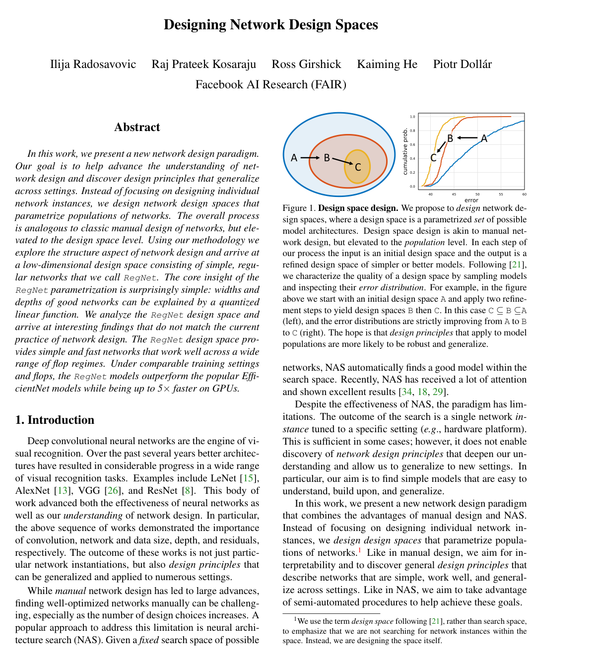
The design space design paradigm iteratively simplifies and improves a population-level architecture space rather than searching for individual model instances. Starting from an initial unconstrained design space (AnyNetX $_\text{A}$ ), successive constraints are applied based on distribution-level empirical evaluation:
1. AnyNetX $_\text{A}$ (16 degrees of freedom, $\sim 1.8 \times 10^{18}$ configurations): Unconstrained baseline where each of the 4 stages has independent block counts $d_i \le 16$ , channel widths $w_i \le 1024$ , bottleneck ratios $b_i \in \{1, 2, 4\}$ , and group widths $g_i \in \{1, 2, \dots, 32\}$ .
2. AnyNetX $_\text{B}$ (13 degrees of freedom, $\sim 6.8 \times 10^{16}$ configurations): Enforces a shared bottleneck ratio $b_i = b$ across all stages $i$ . Error distributions remain virtually identical to AnyNetX $_\text{A}$ .
3. AnyNetX $_\text{C}$ (10 degrees of freedom, $\sim 3.2 \times 10^{14}$ configurations): Enforces a shared group width $g_i = g$ across all stages $i$ , preserving error distribution quality while reducing space complexity by four orders of magnitude.
4. AnyNetX $_\text{D}$ (10 degrees of freedom, $\sim 1.3 \times 10^{13}$ configurations): Enforces monotonically non-decreasing stage widths: $w_{i+1} \ge w_i$ .
5. AnyNetX $_\text{E}$ (10 degrees of freedom, $\sim 5.5 \times 10^{11}$ configurations): Enforces monotonically non-decreasing stage depths: $d_{i+1} \ge d_i$ .
6. RegNetX (6 degrees of freedom, $\sim 3.0 \times 10^{8}$ configurations): Replaces free stage assignments with the 6-parameter quantized linear model $(d, w_0, w_a, w_m, b, g)$ with $d < 64$ , $w_0, w_a < 256$ , $1.5 \le w_m \le 3$ .
Each step simplifies the space, reduces dimensionality, and shifts the model population error distribution toward lower error.
Knowl 3 — Error Empirical Distribution Function for Model Population Quality
definition
The quality of a neural network design space is characterized by sampling $n$ model architectures from the space, training each under identical low-epoch training regimes (e.g., 10 epochs on ImageNet), and evaluating the error empirical distribution function (EDF). For a sample of $n$ models with top-1 classification errors $e_i$ , the error EDF $F(e)$ is defined as:

$F(e) = \frac{1}{n} \sum_{i=1}^n \mathbf{1}[e_i < e]$

where $\mathbf{1}[\cdot]$ is the indicator function. $F(e)$ computes the fraction of sampled models in the design space that achieve a classification error strictly less than $e$ . A design space $S_1$ is considered superior to $S_2$ if its EDF curve is shifted toward lower errors (yielding a lower min error and a lower area under the curve/mean error).
Knowl 4 — RegNet Macro-Architecture and Block Specifications (X and Y Blocks)
model/method
A RegNet model consists of three main components:
1. Stem: A stride-2 $3\times 3$ convolutional layer with fixed output width $w_0 = 32$ channels, followed by Batch Normalization and ReLU, reducing input resolution $r$ to $r/2$ .
2. Body: Composed of 4 sequential stages operating at resolutions $r/4, r/8, r/16, r/32$ . Stage $i$ contains $d_i$ identical blocks of width $w_i$ . The first block of each stage has stride $s = 2$ (halving resolution), while all subsequent blocks in the stage have stride $s = 1$ .
3. Head: Global average pooling layer followed by a fully connected linear layer predicting class logits.
Two primary block structures are used within the body:
- Standard Residual Bottleneck with Group Convolution (X Block): Consists of a $1\times 1$ convolution reducing channels to $w_i / b$ , a $3\times 3$ group convolution with group width $g$ maintaining width $w_i / b$ , and a $1\times 1$ convolution projecting channels back to $w_i$ . Each convolution is followed by Batch Normalization and ReLU. A residual shortcut connection adds the block input to the output (with a stride-2 $1\times 1$ projection on the shortcut when $s=2$ ).
- Squeeze-and-Excitation Residual Block (Y Block): Identical to the X block, but inserts a Squeeze-and-Excitation (SE) module with a channel reduction ratio of $1/4$ directly after the $3\times 3$ group convolution.
Knowl 5 — Empirical Architectural Principles for Optimal Regular Networks
empirical result
Analysis of model populations across complexity regimes (from 200MF to 32GF) yields several structural properties of top-performing regular networks:
- Constant Network Depth: The optimal network depth $d$ remains stable at approximately 20 blocks ( $\,\sim 60$ convolutional layers) across all compute regimes, rather than increasing with FLOPs.
- No Bottleneck ( $b = 1.0$ ): The best models consistently perform best with a bottleneck ratio $b = 1.0$ , rendering the bottleneck compression obsolete.
- Width Factor ( $w_m \approx 2.5$ ): The optimal stage width expansion multiplier is approximately $w_m \approx 2.5$ , outperforming the traditional heuristic of doubling width ( $w_m = 2.0$ ) across stages.
- Late-Stage Capacity Allocation: Top high-compute models concentrate block depth in stage 3 ( $d_3 \gg d_1, d_2$ ) and maintain very few blocks in stage 4 ( $d_4 \in \{1, 2\}$ ).
- Group Width Scaling: Group width $g$ scales upward with compute complexity (e.g., $g=8$ at 200MF up to $g=232$ at 32GF).
- Failure of Inverted Bottlenecks and Resolution Scaling: Inverted bottleneck configurations ( $b < 1$ ) and depthwise convolutions ( $g = 1$ ) degrade accuracy compared to $b=1$ with $g > 1$ . Furthermore, scaling input image resolution beyond $224\times 224$ under fixed FLOP constraints degrades top-1 accuracy.
Knowl 6 — Activation Complexity and Hardware Accelerator Efficiency
empirical result
Network activation count is defined as the total number of elements in output tensors across all convolutional layers in the network. On memory-bandwidth-bound hardware accelerators (such as NVIDIA V100 GPUs), inference latency exhibits a stronger linear correlation with activations ( $r = 0.897$ ) than with multiply-add operations/FLOPs ( $r = 0.643$ ).

In RegNet architectures, network activations scale with the square root of compute ( $\,\text{Activations} \propto \sqrt{\text{FLOPs}}\,)$ , whereas parameter count scales linearly ( $\,\text{Params} \propto \text{FLOPs}\,)$ . In contrast, architectures like EfficientNet scale depth, width, and input resolution concurrently, causing activation count to scale linearly with FLOPs ( $\text{Activations} \propto \text{FLOPs}$ ). Consequently, for comparable or superior ImageNet top-1 error under identical 100-epoch training setups, RegNet models run up to $5\times$ faster than EfficientNet on GPU (e.g., RegNetX-8.0GF executes inference in 94 ms vs 504 ms for EfficientNet-B5).

Knowl 7 — Top-Performing RegNetX and RegNetY Model Specifications and ImageNet Benchmarks

data/table

Top RegNetX and RegNetY models identified via the quantized linear parameterization, evaluated on ImageNet (trained for 100 epochs with standard SGD without training-time regularizations/enhancements, evaluated at resolution $224\times 224$ ):

Model	FLOPs (B)	Params (M)	Acts (M)	Infer (ms)	Top-1 Error (%)
RegNetX-200MF	0.2	2.7	2.2	10	$31.1 \pm 0.09$
RegNetX-400MF	0.4	5.2	3.1	15	$27.3 \pm 0.15$
RegNetX-600MF	0.6	6.2	4.0	17	$25.9 \pm 0.03$
RegNetX-800MF	0.8	7.3	5.1	21	$24.8 \pm 0.09$
RegNetX-1.6GF	1.6	9.2	7.9	33	$23.0 \pm 0.13$
RegNetX-3.2GF	3.2	15.3	11.4	57	$21.7 \pm 0.08$
RegNetX-4.0GF	4.0	22.1	12.2	69	$21.4 \pm 0.19$
RegNetX-6.4GF	6.5	26.2	16.4	92	$20.8 \pm 0.07$
RegNetX-8.0GF	8.0	39.6	14.1	94	$20.7 \pm 0.07$
RegNetX-12GF	12.1	46.1	21.4	137	$20.3 \pm 0.04$
RegNetX-16GF	15.9	54.3	25.5	168	$20.0 \pm 0.11$
RegNetX-32GF	31.7	107.8	36.3	318	$19.5 \pm 0.12$
RegNetY-200MF	0.2	3.2	2.2	11	$29.6 \pm 0.11$
RegNetY-400MF	0.4	4.3	3.9	19	$25.9 \pm 0.16$
RegNetY-600MF	0.6	6.1	4.3	19	$24.5 \pm 0.07$
RegNetY-800MF	0.8	6.3	5.2	22	$23.7 \pm 0.03$
RegNetY-1.6GF	1.6	11.2	8.0	39	$22.0 \pm 0.08$
RegNetY-3.2GF	3.2	19.4	11.3	67	$21.0 \pm 0.05$
RegNetY-4.0GF	4.0	20.6	12.3	68	$20.6 \pm 0.08$
RegNetY-6.4GF	6.4	30.6	16.4	104	$20.1 \pm 0.04$
RegNetY-8.0GF	8.0	39.2	18.0	113	$20.1 \pm 0.09$
RegNetY-12GF	12.1	51.8	21.4	150	$19.7 \pm 0.06$
RegNetY-16GF	15.9	83.6	23.0	189	$19.6 \pm 0.16$
RegNetY-32GF	32.3	145.0	30.3	319	$19.0 \pm 0.12$

Inference latency is measured for batch size 64 on an NVIDIA V100 GPU.

Knowl 8 — Group Width and Channel Width Compatibility Algorithm
algorithm
When sampling arbitrary stage channel widths $w$ and group widths $g$ , the channel count may not be divisible by $g$ . To guarantee valid group convolution configurations without significantly altering the sampled width parameter, widths and group sizes are adjusted using the following procedure:
Input: Proposed channel width $w$ , proposed group width $g$
Output: Compatible channel width $w^*$ , compatible group width $g^*$
if $g > w$ then
     $g^* = w$
     $w^* = w$
else
     $w^* = \text{round}(w / g) \times g$
     $g^* = g$
end if
return $w^*, g^*$
For bottleneck blocks with bottleneck ratio $b$ , this algorithm is applied to the bottleneck channel width $w / b$ . The adjustment ensures that the final width $w^*$ deviates from the initial width $w$ by at most a factor of $1/3$ .
Knowl 9 — Swish and ReLU Interaction with Group Convolutions
empirical result
Evaluating the Swish activation function versus standard ReLU in RegNet architectures reveals an interaction dependent on group convolution structure:
- In standard RegNet models with group width $g > 1$ , Swish performs better than ReLU in low-compute regimes (e.g., $28.7\%$ vs $29.8\%$ error at 400MF), but performs worse than ReLU in higher-compute regimes (e.g., $22.6\%$ vs $22.1\%$ error at 6.4GF).
- When models are restricted to depthwise convolutions ( $g = 1$ ), Swish substantially outperforms ReLU across all compute regimes.
This demonstrates that the effectiveness of Swish over ReLU observed in popular mobile networks is tied to the use of depthwise separable convolutions ( $g = 1$ ) rather than a universal superiority over ReLU.

Coverage note — ImageNetV2 generalization experiments, hyperparameter sweeps verifying standard optimization stability across FLOPs (lr=0.1, wd=5e-5), and intermediate non-residual V/VR block ablations were omitted as they serve solely to corroborate the main architectural findings.

References

1.F. Chollet. Xception: Deep learning with depthwise separable convolutions. In CVPR, 2017. 7
2.E. D. Cubuk, B. Zoph, D. Mane, V. Vasudevan, and Q. V. Le. AutoAugment: Learning augmentation policies from data. arXiv:1805.09501, 2018. 8, 11
3.J. Deng, W. Dong, R. Socher, L.-J. Li, K. Li, and L. Fei-Fei. Imagenet: A large-scale hierarchical image database. In CVPR, 2009. 2, 3, 8, 10
4.T. DeVries and G. W. Taylor. Improved regularization of convolutional neural networks with cutout. arXiv:1708.04552, 2017. 8
5.B. Efron and R. J. Tibshirani. An introduction to the bootstrap. CRC press, 1994. 3
6.P. Goyal, P. Dollár, R. Girshick, P. Noordhuis, L. Wesolowski, A. Kyrola, A. Tulloch, Y. Jia, and K. He. Accurate, large minibatch sgd: Training imagenet in 1 hour. arXiv:1706.02677, 2017. 11
7.K. He, X. Zhang, S. Ren, and J. Sun. Delving deep into rectifiers: Surpassing human-level performance on imagenet classification. In ICCV, 2015. 2
8.K. He, X. Zhang, S. Ren, and J. Sun. Deep residual learning for image recognition. In CVPR, 2016. 1, 2, 3, 9
9.A. G. Howard, M. Zhu, B. Chen, D. Kalenichenko, W. Wang, T. Weyand, M. Andreetto, and H. Adam. Mobilenets: Efficient convolutional neural networks for mobile vision applications. arXiv:1704.04861, 2017. 2, 8
10.J. Hu, L. Shen, and G. Sun. Squeeze-and-excitation networks. In CVPR, 2018. 7
11.G. Huang, Z. Liu, L. Van Der Maaten, and K. Q. Weinberger. Densely connected convolutional networks. In CVPR, 2017. 2
12.S. Ioffe and C. Szegedy. Batch normalization: Accelerating deep network training by reducing internal covariate shift. In ICML, 2015. 4
13.A. Krizhevsky, I. Sutskever, and G. E. Hinton. Imagenet classification with deep convolutional neural networks. In NIPS, 2012. 1, 2
14.G. Larsson, M. Maire, and G. Shakhnarovich. Fractalnet: Ultra-deep neural networks without residuals. In ICLR, 2017. 8, 11
15.Y. LeCun, B. Boser, J. S. Denker, D. Henderson, R. E. Howard, W. Hubbard, and L. D. Jackel. Backpropagation applied to handwritten zip code recognition. Neural computation, 1989. 1
16.C.-Y. Lee, S. Xie, P. Gallagher, Z. Zhang, and Z. Tu. Deeply-supervised nets. In AISTATS, 2015. 8
17.C. Liu, B. Zoph, M. Neumann, J. Shlens, W. Hua, L.-J. Li, L. Fei-Fei, A. Yuille, J. Huang, and K. Murphy. Progressive neural architecture search. In ECCV, 2018. 2, 8
18.H. Liu, K. Simonyan, and Y. Yang. Darts: Differentiable architecture search. In ICLR, 2019. 1, 2, 8
19.N. Ma, X. Zhang, H.-T. Zheng, and J. Sun. Shufflenet v2: Practical guidelines for efficient cnn architecture design. In ECCV, 2018. 8
20.H. Pham, M. Y. Guan, B. Zoph, Q. V. Le, and J. Dean. Efficient neural architecture search via parameter sharing. In ICML, 2018. 2
21.I. Radosavovic, J. Johnson, S. Xie, W.-Y. Lo, and P. Dollár. On network design spaces for visual recognition. In ICCV, 2019. 1, 2, 3, 4, 11
22.P. Ramachandran, B. Zoph, and Q. V. Le. Searching for activation functions. arXiv:1710.05941, 2017. 10
23.E. Real, A. Aggarwal, Y. Huang, and Q. V. Le. Regularized evolution for image classifier architecture search. In AAAI, 2019. 2, 8
24.B. Recht, R. Roelofs, L. Schmidt, and V. Shankar. Do imagenet classifiers generalize to imagenet? arXiv:1902.10811, 2019. 2, 10
25.M. Sandler, A. Howard, M. Zhu, A. Zhmoginov, and L.-C. Chen. Mobilenetv2: Inverted residuals and linear bottlenecks. In CVPR, 2018. 2, 7, 8
26.K. Simonyan and A. Zisserman. Very deep convolutional networks for large-scale image recognition. In ICLR, 2015. 1, 2
27.C. Szegedy, W. Liu, Y. Jia, P. Sermanet, S. Reed, D. Anguelov, D. Erhan, V. Vanhoucke, and A. Rabinovich. Going deeper with convolutions. In CVPR, 2015. 2
28.C. Szegedy, V. Vanhoucke, S. Ioffe, J. Shlens, and Z. Wojna. Rethinking the inception architecture for computer vision. In CVPR, 2016. 2
29.M. Tan and Q. V. Le. Efficientnet: Rethinking model scaling for convolutional neural networks. ICML, 2019. 1, 2, 7, 9, 10, 11
30.T. Tieleman and G. Hinton. Lecture 6.5-rmsprop: Divide the gradient by a running average of its recent magnitude. Coursera: Neural networks for machine learning, 2012. 11
31.S. Xie, R. Girshick, P. Dollár, Z. Tu, and K. He. Aggregated residual transformations for deep neural networks. In CVPR, 2017. 2, 4, 9
32.S. Zagoruyko and N. Komodakis. Wide residual networks. In BMVC, 2016. 2
33.X. Zhang, X. Zhou, M. Lin, and J. Sun. Shufflenet: An extremely efficient convolutional neural network for mobile devices. In CVPR, 2018. 8
34.B. Zoph and Q. V. Le. Neural architecture search with reinforcement learning. In ICLR, 2017. 1
35.B. Zoph, V. Vasudevan, J. Shlens, and Q. V. Le. Learning transferable architectures for scalable image recognition. In CVPR, 2018. 2, 8

Citation

MLA

Radosavovic, I., et al. “Designing Network Design Spaces”. arXiv, 2020, http://arxiv.org/abs/2003.13678v1.

APA

Radosavovic, I., Kosaraju, R. P., Girshick, R., He, K., & Dollár, P. (2020). Designing Network Design Spaces. arXiv. http://arxiv.org/abs/2003.13678v1

Chicago

Radosavovic, I., R. P. Kosaraju, R. Girshick, K. He, and P. Dollár. 2020. “Designing Network Design Spaces”. arXiv. http://arxiv.org/abs/2003.13678v1.

Harvard

Radosavovic, I. et al. (2020) “Designing Network Design Spaces”, arXiv [Preprint]. Available at: http://arxiv.org/abs/2003.13678v1.

Vancouver

1. Radosavovic I, Kosaraju RP, Girshick R, He K, Dollár P (2020) Designing Network Design Spaces. arXiv

BibTeX

@article{radosavovic2020designing,
  title = {Designing Network Design Spaces},
  author = {Radosavovic, Ilija and Kosaraju, Raj Prateek and Girshick, Ross and He, Kaiming and Dollár, Piotr},
  year = {2020},
  journal = {arXiv},
  url = {http://arxiv.org/abs/2003.13678v1},
  eprint = {2003.13678}
}

Metadata:arXiv

Source Code

This paper has an official code repository available. Click below to access the source code.

View Repository

Access the Paper

This paper is available from its original source. Click below to access the PDF.

Open PDF

License: IEEE

Designing Network Design Spaces

Abstract

Topics

Keywords

Table of Contents

Knowls

Knowl 1 — RegNet Quantized Linear Width and Depth Parameterization

Knowl 2 — Design Space Design via Stepwise AnyNet Subspace Refinement

Knowl 3 — Error Empirical Distribution Function for Model Population Quality

Knowl 4 — RegNet Macro-Architecture and Block Specifications (X and Y Blocks)

Knowl 5 — Empirical Architectural Principles for Optimal Regular Networks

Knowl 6 — Activation Complexity and Hardware Accelerator Efficiency