SplatAD: Real-Time Lidar and Camera Rendering with 3D Gaussian Splatting for Autonomous Driving

Georg HessCarl LindstrmMaryam FatemiChristoffer PeterssonLennart Svensson

article2025CVPR88 citations

Introduces the first 3D Gaussian Splatting framework for simultaneous real-time rendering of both camera and lidar data in dynamic autonomous driving scenes, accurately modeling sensor-specific effects like rolling shutter and ray dropouts while rendering an order of magnitude faster than NeRF-based alternatives.

Listen

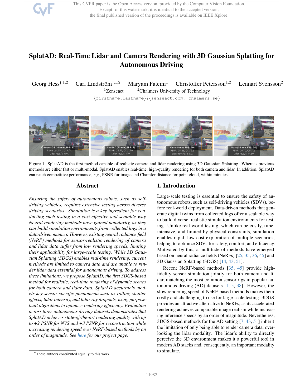
Autonomous driving systems rely heavily on simulation to safely and affordably test complex traffic scenarios before deploying vehicles in the real world. While data-driven neural rendering methods can generate realistic simulation environments from logged sensor data, existing approaches face a major trade-off. Prior neural radiance field methods accurately model both camera images and lidar point clouds but suffer from slow rendering speeds, making large-scale simulation expensive. Conversely, newer real-time methods based on 3D Gaussian Splatting achieve rapid rendering for camera views but lack native support for lidar, an essential sensor modality for 3D spatial perception.

The article demonstrates SplatAD, a unified framework using 3D Gaussian Splatting that delivers real-time, sensor-realistic rendering of both camera images and lidar point clouds in dynamic traffic environments. The method models both static surroundings and moving actors within a single scene representation, employing tailored acceleration algorithms and sensor-specific compensation to handle hardware characteristics such as rolling shutter distortions, lidar beam dropouts, and intensity variations.

To evaluate this approach, the authors conducted experiments across three standard autonomous driving benchmarks: PandaSet, Argoverse 2, and nuScenes. The evaluations assessed novel view synthesis and full scene reconstruction against established baselines, measuring image realism, 3D point cloud accuracy, extrapolation to new vehicle paths, and rendering throughput using full-resolution data on a single graphics processing unit.

The findings show that SplatAD outperforms existing methods in both speed and fidelity. SplatAD renders camera images at over 100 megapixels per second—roughly 10 times faster than prior multi-modal neural radiance fields—while delivering superior image quality, achieving improvements of up to 2 to 3 peak signal-to-noise ratio points. For lidar simulation, SplatAD achieves up to 18 times faster rendering than leading ray-tracing methods while accurately capturing point cloud structure and ray dropouts. Furthermore, ablation analyses confirm that modeling rolling shutter distortions directly prevents structural errors, while a lightweight neural decoding network enhances high-frequency texture details such as road surfaces.

These results demonstrate that high-throughput simulation no longer requires sacrificing multi-modal realism or geometric accuracy. By reducing rendering time by an order of magnitude without compromising sensor fidelity, the approach allows engineering teams to drastically scale up closed-loop simulation and safety validation pipelines at a lower computational cost. Organizations developing automated driving systems should consider integrating spherical coordinate splatting and rolling shutter compensation into their simulation stacks to enhance testing capacity.

Decision-makers should note that the current implementation treats all dynamic objects as rigid bounding boxes, meaning it cannot yet model the non-rigid motion of pedestrians or cyclists. Additionally, while the results provide high confidence across the tested benchmarks, generalizing to extreme sensor path shifts beyond the original vehicle trajectory remains a challenge. Future development should focus on incorporating non-rigid actor models and generative image priors to further improve scenario modification capabilities.

arXiv: 2411.16816

No sufficiently relevant recommendations were found.
Cover for SplatAD: Real-Time Lidar and Camera Rendering with 3D Gaussian Splatting for Autonomous Driving

Abstract

Ensuring the safety of autonomous robots, such as self-driving vehicles, requires extensive testing across diverse driving scenarios. Simulation is a key ingredient for conducting such testing in a cost-effective and scalable way. Neural rendering methods have gained popularity, as they can build simulation environments from collected logs in a data-driven manner. However, existing neural radiance field (NeRF) methods for sensor-realistic rendering of camera and lidar data suffer from low rendering speeds, limiting their applicability for large-scale testing. While 3D Gaussian Splatting (3DGS) enables real-time rendering, current methods are limited to camera data and are unable to render lidar data essential for autonomous driving. To address these limitations, we propose SplatAD, the first 3DGS-based method for realistic, real-time rendering of dynamic scenes for both camera and lidar data. SplatAD accurately models key sensor-specific phenomena such as rolling shutter effects, lidar intensity, and lidar ray dropouts, using purpose-built algorithms to optimize rendering efficiency. Evaluation across three autonomous driving datasets demonstrates that SplatAD achieves state-of-the-art rendering quality with up to +2 PSNR for NVS and +3 PSNR for reconstruction while increasing rendering speed over NeRF-based methods by an order of magnitude. See here for our project page.

Table of Contents

  • 1. Introduction
  • 2. Related work
  • 3. Method
  • 3.1. Scene representation
  • 3.2. Camera rendering
  • 3.3. Lidar rendering
  • 3.4. Optimization and implementation
  • 4. Experiments
  • 4.1. Image rendering
  • 4.2. Lidar rendering
  • 4.3. Ablations
  • 5. Conclusion
  • Acknowledgements
  • References

Knowls

  1. Knowl 1 — Unified multimodal Gaussian representation

    model/method

    SplatAD represents an autonomous-driving scene with a single explicit set of translucent 3D Gaussians that can be rendered into both camera images and lidar point clouds. Each Gaussian has a learnable opacity o∈(0,1)o\in(0,1), mean μ∈R3\boldsymbol{\mu}\in\mathbb{R}^3, covariance Σ∈R3×3\boldsymbol{\Sigma}\in\mathbb{R}^{3\times3} parameterized by a scale vector and quaternion, a learnable base RGB color frgb∈R3\mathbf{f}^{\mathrm{rgb}}\in\mathbb{R}^3, and a learnable feature vector f∈RDf\mathbf{f}\in\mathbb{R}^{D_f}. Unlike standard 3D Gaussian Splatting, SplatAD replaces spherical harmonics with these features and adds a learned embedding for each sensor, allowing one representation to model view-dependent camera appearance, lidar intensity, ray dropouts, and sensor-specific exposure or appearance.

    The rendering pipeline composes static and dynamic Gaussians at a requested capture time, projects them into either camera or lidar coordinates, assigns them to modality-specific tiles, compensates their positions for rolling shutter, alpha-blends their features, and decodes the blended features into an image or lidar range, intensity, and ray-drop probability. This unified rasterization design is the central mechanism that provides multimodal rendering at 3DGS-like inference speeds.

  2. Knowl 2 — Dynamic scene-graph composition with learnable motion corrections

    model/method

    SplatAD decomposes a driving scene into a static background and dynamic actors. Each actor is represented by a 3D axis-aligned bounding box, a sequence of SE(3)\mathrm{SE}(3) poses, an actor identifier assigned to its Gaussians, and a velocity initialized from pose differences. Gaussian means and covariances belonging to an actor are stored in that actor's local coordinate system; at capture time tt, they are transformed into world coordinates using the actor pose. Static-background Gaussians remain in world coordinates.

    Because detector and tracker poses can be inaccurate, SplatAD jointly learns pose offsets for each actor and a velocity offset for each actor. The resulting composed Gaussian set permits changing both the ego-vehicle pose and actor poses during rendering. The method treats every dynamic actor as rigid, so within-actor non-rigid motion is not represented.

  3. Knowl 3 — Camera rasterization with dynamic rolling-shutter compensation

    model/method

    For a camera capture, SplatAD transforms each Gaussian into camera coordinates, applies perspective projection to obtain an image-space mean μiI∈R2\boldsymbol{\mu}_i^I\in\mathbb{R}^2, and transforms its covariance with the projection Jacobian JI\mathbf{J}^I as ΣiI=JIΣiC(JI)⊤\boldsymbol{\Sigma}_i^I=\mathbf{J}^I\boldsymbol{\Sigma}_i^C(\mathbf{J}^I)^\top. Gaussians are culled using a 99%-confidence axis-aligned bounding box, assigned to overlapping 16×1616\times16-pixel tiles, and sorted by the depth of their camera-space means.

    For a Gaussian, camera motion and actor motion induce the image-space velocity

    viI=JI(−ωC×μiC−vC+vi,dyn)∈R2,\mathbf{v}_i^I=\mathbf{J}^I\left(-\boldsymbol{\omega}_C\times\boldsymbol{\mu}_i^C-\mathbf{v}_C+\mathbf{v}_{i,\mathrm{dyn}}\right)\in\mathbb{R}^2,

    where ωC,vC∈R3\boldsymbol{\omega}_C,\mathbf{v}_C\in\mathbb{R}^3 are the camera angular and linear velocities in camera coordinates, μiC\boldsymbol{\mu}_i^C is the Gaussian mean in camera coordinates, and vi,dyn\mathbf{v}_{i,\mathrm{dyn}} is the actor-induced Gaussian velocity transformed into camera coordinates; it is zero for static-background Gaussians. If pvp_v is the vertical pixel coordinate, HH is image height, and trst_{\mathrm{rs}} is the time between the first and last image rows, the pixel's capture-time offset from the image midpoint is

    tpix=(pvH−0.5)trs.t_{\mathrm{pix}}=\left(\frac{p_v}{H}-0.5\right)t_{\mathrm{rs}}.

    For a pixel p\mathbf{p}, the rolling-shutter-corrected Gaussian displacement is Δi=p−(μiI+viItpix)\boldsymbol{\Delta}_i=\mathbf{p}-(\boldsymbol{\mu}_i^I+\mathbf{v}_i^I t_{\mathrm{pix}}). Its alpha contribution uses the 3DGS+EWA form with smoothing constant s=0.3s=0.3:

    αi=∣ΣiI∣∣ΣiI+sI∣ oiexp⁡[−12Δi⊤(ΣiI+sI)−1Δi],\alpha_i=\sqrt{\frac{|\boldsymbol{\Sigma}_i^I|}{|\boldsymbol{\Sigma}_i^I+s\mathbf{I}|}}\,o_i\exp\left[-\frac{1}{2}\boldsymbol{\Delta}_i^\top(\boldsymbol{\Sigma}_i^I+s\mathbf{I})^{-1}\boldsymbol{\Delta}_i\right],

    where I\mathbf{I} is the 2×22\times2 identity matrix. RGB colors and features are composited in depth order using

    [Fprgb,Fp]=∑i[firgb,fi]αi∏j<i(1−αj).[\mathbf{F}^{\mathrm{rgb}}_{\mathbf{p}},\mathbf{F}_{\mathbf{p}}]=\sum_i[\mathbf{f}^{\mathrm{rgb}}_i,\mathbf{f}_i]\alpha_i\prod_{j<i}(1-\alpha_j).

    The image-space bounding box is enlarged by ∥viI∥trs/2\|\mathbf{v}_i^I\|t_{\mathrm{rs}}/2 and by a learned sensor-time offset, so culling and tile intersections include motion during exposure. A small CNN then receives the rasterized feature map F\mathbf{F}, ray directions d\mathbf{d}, and a camera-specific embedding e\mathbf{e}, and predicts per-pixel affine parameters M\mathbf{M} and b\mathbf{b}:

    (M,b)=CNN(concat(F,d,e)),I=(1+M)⊙Frgb+b.(\mathbf{M},\mathbf{b})=\mathrm{CNN}(\mathrm{concat}(\mathbf{F},\mathbf{d},\mathbf{e})),\qquad \mathbf{I}=(1+\mathbf{M})\odot\mathbf{F}^{\mathrm{rgb}}+\mathbf{b}.

    The CNN is used instead of an MLP because it models high-frequency textures more efficiently and improves image sharpness and color fidelity.

  4. Knowl 4 — Spherical lidar Gaussian rasterization

    model/method

    SplatAD renders spinning lidar directly in spherical coordinates rather than approximating a 360-degree lidar with several depth cameras. For a Gaussian with lidar-coordinate mean (x,y,z)⊤(x,y,z)^\top and covariance ΣL\boldsymbol{\Sigma}^L, the spherical mean is

    μS=[ϕωr]=[atan2⁡(y,x)arcsin⁡(z/r)x2+y2+z2],\boldsymbol{\mu}^S= \begin{bmatrix}\phi\\\omega\\r\end{bmatrix} = \begin{bmatrix} \operatorname{atan2}(y,x)\\ \arcsin(z/r)\\ \sqrt{x^2+y^2+z^2} \end{bmatrix},

    where ϕ\phi is azimuth, ω\omega is elevation, and rr is range. The spherical covariance is ΣS=JSΣL(JS)⊤\boldsymbol{\Sigma}^S=\mathbf{J}^S\boldsymbol{\Sigma}^L(\mathbf{J}^S)^\top, with ρ=x2+y2\rho=\sqrt{x^2+y^2} and

    JS=[−y/(x2+y2)x/(x2+y2)0−xz/(r2ρ)−yz/(r2ρ)ρ/r2x/ry/rz/r].\mathbf{J}^S= \begin{bmatrix} -y/(x^2+y^2) & x/(x^2+y^2) & 0\\ -xz/(r^2\rho) & -yz/(r^2\rho) & \rho/r^2\\ x/r & y/r & z/r \end{bmatrix}.

    Lidar rolling shutter is handled with the spherical velocity vS=JS(−ωL×μL−vL+vdyn)\mathbf{v}^S=\mathbf{J}^S(-\boldsymbol{\omega}_L\times\boldsymbol{\mu}^L-\mathbf{v}_L+\mathbf{v}_{\mathrm{dyn}}), where ωL\boldsymbol{\omega}_L and vL\mathbf{v}_L are lidar angular and linear velocities and vdyn\mathbf{v}_{\mathrm{dyn}} is the actor-induced velocity in lidar coordinates. The azimuth and elevation extents are enlarged using the first two components of vStrs/2\mathbf{v}^S t_{\mathrm{rs}}/2.

    The lidar rasterizer uses tiles containing a fixed number of vertical laser diodes and a fixed azimuth resolution. Horizontal tile intersections wrap around 360 degrees; vertical intersections are computed from the lidar's sorted, potentially non-equidistant elevation boundaries. Gaussians are sorted by their spherical range. This avoids the excessive computation caused by representing sparse, non-equidistant lidar measurements as a dense depth image.

    Each lidar ray supplies azimuth, elevation, and capture time to a CUDA thread. The Gaussian features are alpha-blended using the same transmittance compositing principle as camera rendering, with the EWA smoothing scale set to the geometric mean of the lidar's vertical and horizontal beam divergences. The blended features and ray direction are decoded by a small MLP into lidar intensity and ray-drop probability. The range decoder uses the rolling-shutter-corrected Gaussian range ri,rs=ri+vr,iStlr_{i,\mathrm{rs}}=r_i+v^S_{r,i}t_l, where vr,iSv^S_{r,i} is the range component of the relative velocity and tlt_l is the ray's time offset from the scan midpoint. Expected range is used for training; at inference, SplatAD outputs the rolling-shutter-corrected range of the first Gaussian for which cumulative opacity exceeds 0.50.5, yielding a median depth that avoids depths falling between surfaces.

  5. Knowl 5 — Joint training objective and efficient implementation

    algorithm

    SplatAD jointly optimizes Gaussian parameters, actor corrections, sensor embeddings, decoders, and sensor-motion quantities with

    L=λrL1+(1−λr)LSSIM+λdepthLdepth+λlosLlos+λintensLinten+λraydropLBCE+λMCMCLMCMC.\mathcal{L}=\lambda_r\mathcal{L}_1+(1-\lambda_r)\mathcal{L}_{\mathrm{SSIM}}+\lambda_{\mathrm{depth}}\mathcal{L}_{\mathrm{depth}}+\lambda_{\mathrm{los}}\mathcal{L}_{\mathrm{los}}+\lambda_{\mathrm{intens}}\mathcal{L}_{\mathrm{inten}}+\lambda_{\mathrm{raydrop}}\mathcal{L}_{\mathrm{BCE}}+\lambda_{\mathrm{MCMC}}\mathcal{L}_{\mathrm{MCMC}}.

    Here L1\mathcal{L}_1 and LSSIM\mathcal{L}_{\mathrm{SSIM}} compare rendered and target images; Ldepth\mathcal{L}_{\mathrm{depth}} and Linten\mathcal{L}_{\mathrm{inten}} are squared errors on expected lidar range and intensity; Llos\mathcal{L}_{\mathrm{los}} penalizes opacity accumulated before the ground-truth lidar range; LBCE\mathcal{L}_{\mathrm{BCE}} trains ray-drop probabilities using binary cross-entropy; and LMCMC\mathcal{L}_{\mathrm{MCMC}} is the opacity and scale regularizer associated with the adopted Gaussian MCMC densification strategy. The λ\lambda values are loss weights.

    Gaussians are initialized from lidar points and random points. Lidar points inside actor boxes are assigned to those actors, and all lidar points are projected into their nearest camera image to initialize color. Additional random points are sampled uniformly within the lidar range and linearly in disparity beyond the lidar range. SplatAD uses MCMC-based Gaussian growth instead of standard 3DGS splitting and densification, allowing a predictable maximum Gaussian count and improving far-field quality.

    Forward and backward passes for lidar projection, lidar rasterization, and rolling-shutter compensation use custom CUDA kernels. The model is trained for 30,000 Adam iterations, requiring approximately one hour on a single NVIDIA A100.

  6. Knowl 6 — Cross-dataset evaluation protocol

    experimental setup

    SplatAD is evaluated on PandaSet, Argoverse2, and nuScenes using the same hyperparameters across datasets. The experiments use six cameras for PandaSet and nuScenes and seven ring cameras for Argoverse2; black-and-white stereo cameras are excluded, and some views are slightly cropped to remove the ego-vehicle. Ten challenging sequences per dataset are used, covering varied illumination, dynamic actors, and vehicle velocities. For novel-view synthesis, every other frame is used for training and the remaining frames are held out at full resolution.

    The comparison methods are UniSim and NeuRAD (NeRF-based) and PVG, Street Gaussians, and OmniRE (3DGS-based). Camera quality is evaluated with PSNR, SSIM, and LPIPS, and camera speed with megapixels per second. Lidar quality is evaluated with median squared depth error, RMSE intensity error, ray-drop accuracy, and Chamfer distance, and lidar speed with millions of rays per second. Unlike the depth-image baselines, SplatAD predicts ranges for missing rays and filters them using its predicted ray-drop probability.

    For reconstruction, all data from a PandaSet sequence are used for training and evaluation is performed on the same views, with sensor-pose optimization enabled for all methods. Extrapolation is tested by shifting the ego vehicle horizontally or vertically and by shifting and rotating dynamic actors; the resulting images are compared with DINOv2 feature Fréchet distance, where lower is better.

  7. Knowl 7 — Image novel-view synthesis results

    data/table

    The image NVS comparison measures visual quality on held-out frames and rendering efficiency. SplatAD is the best method on every reported image metric for all three datasets, while also rendering faster than both NeRF and other 3DGS methods. PSNR and SSIM are higher-is-better, LPIPS is lower-is-better, MP/s is megapixels per second, and Train is training time in hours.

    Dataset Method PSNR↑\uparrow SSIM↑\uparrow LPIPS↓\downarrow MP/s↑\uparrow Train (H)↓\downarrow
    PandaSet UniSim 23.12 0.682 0.360 11.5 0.9
    NeuRAD 25.80 0.753 0.250 9.7 1.3
    PVG 24.01 0.712 0.452 22.6 1.6
    Street-GS 24.73 0.745 0.314 63.1 2.3
    OmniRE 24.71 0.745 0.315 53.6 2.6
    SplatAD 26.70 0.814 0.193 104.1 1.0
    Argo2 UniSim 22.35 0.655 0.458 10.0 1.1
    NeuRAD 26.18 0.721 0.310 9.7 1.3
    PVG 24.47 0.712 0.502 19.7 2.5
    Street-GS 25.52 0.754 0.374 92.8 2.6
    OmniRE 25.61 0.753 0.375 75.6 3.0
    SplatAD 28.40 0.826 0.271 133.8 1.2
    nuScenes UniSim 22.66 0.743 0.414 13.3 0.7
    NeuRAD 26.17 0.790 0.312 11.8 1.1
    PVG 24.94 0.768 0.497 18.8 1.4
    Street-GS 25.54 0.799 0.375 57.9 1.6
    OmniRE 25.50 0.798 0.386 46.9 1.9
    SplatAD 27.53 0.849 0.302 104.3 1.2

    Relative to NeuRAD, SplatAD improves PSNR by 0.90, 2.22, and 1.36 on PandaSet, Argo2, and nuScenes, respectively, while increasing image rendering speed by approximately one order of magnitude.

  8. Knowl 8 — Lidar rendering and PandaSet reconstruction results

    data/table

    SplatAD produces lidar point clouds with quality comparable to the accurate ray-tracing-based NeuRAD renderer while being substantially faster, and it improves on the depth-image-based 3DGS baselines. A superscript §\S denotes results evaluated without missing points because the corresponding baseline cannot infer ray dropouts. Depth is median squared error, intensity is RMSE, CD is Chamfer distance, and MR/s is millions of rays per second.

    Dataset Method Depth↓\downarrow Intensity↓\downarrow Drop acc.↑\uparrow CD↓\downarrow MR/s↑\uparrow
    PandaSet UniSim 0.08 0.086 – 10.3§^{\S} 0.9
    NeuRAD 0.01 0.063 96.2 1.9 1.1
    PVG 38.74 – – 125.2§^{\S} 0.3
    Street-GS 6.18 – – 37.3§^{\S} 0.8
    OmniRE 2.88 – – 29.8§^{\S} 0.6
    SplatAD 0.01 0.059 96.7 1.6 19.5
    Argo2 UniSim 0.18 0.081 – 29.2§^{\S} 0.7
    NeuRAD 0.02 0.058 92.2 2.6 0.9
    SplatAD 0.02 0.052 92.6 2.8 9.5
    nuScenes UniSim 0.06 0.063 – 52.2§^{\S} 1.0
    NeuRAD 0.01 0.042 93.1 6.3 1.1
    PVG 10.34 – – 77.9§^{\S} 0.05
    Street-GS 1.56 – – 4.5§^{\S} 0.2
    OmniRE 1.71 – – 4.6§^{\S} 0.1
    SplatAD 0.02 0.036 93.8 1.7 5.7

    On the PandaSet reconstruction task, where training and evaluation use the same views, SplatAD also achieves the strongest image and lidar quality while remaining fast:

    Method PSNR SSIM LPIPS Depth Intensity Drop acc. CD Camera MP/s Lidar MR/s Train (H)
    UniSim 23.18 0.684 0.362 0.06 0.087 – 10.2§^{\S} 11.1 0.8 0.8
    NeuRAD 26.76 0.778 0.233 0.03 0.074 96.1 1.7 9.8 1.1 1.3
    PVG 25.35 0.752 0.423 53.18 – – 150.8§^{\S} 23.6 0.3 1.6
    Street-GS 26.68 0.808 0.293 3.27 – – 27.9§^{\S} 65.7 0.8 2.2
    OmniRE 26.68 0.808 0.295 3.80 – – 33.5§^{\S} 56.7 0.6 2.4
    SplatAD 29.74 0.893 0.175 0.02 0.053 97.4 1.6 104.1 17.4 1.0

    The paper reports lidar speedups of up to 18×18\times over NeuRAD and finds that direct spherical rasterization is both faster and more accurate than synthesizing lidar through virtual depth cameras.

  9. Knowl 9 — Component ablations and pose extrapolation

    empirical result

    Ablations averaged over ten sequences from each of the three datasets show that the principal sensor-modeling components improve quality without materially reducing speed. The full model obtains PSNR 27.5427.54, SSIM 0.8300.830, LPIPS 0.2550.255, depth error 0.020.02, Chamfer distance 2.02.0, camera speed 114.1114.1 MP/s, and lidar speed 11.411.4 MR/s.

    Variant PSNR↑\uparrow SSIM↑\uparrow LPIPS↓\downarrow Depth↓\downarrow CD↓\downarrow Camera MP/s↑\uparrow Lidar MR/s↑\uparrow
    Full model 27.54 0.830 0.255 0.02 2.0 114.1 11.4
    Without camera rolling shutter 27.48 0.828 0.258 0.02 2.1 116.3 11.5
    Without CNN decoder 27.23 0.824 0.264 0.02 2.2 178.0 11.6
    Without EWA antialiasing 27.60 0.828 0.268 0.02 1.5 114.5 11.0
    Without appearance embeddings 27.28 0.824 0.264 0.02 2.1 121.0 11.5
    Without velocity optimization 27.55 0.830 0.257 0.02 114.1 11.4
    Without lidar rolling shutter 27.42 0.827 0.260 0.03 2.1 114.2 12.2
    Without MCMC 27.35 0.826 0.259 0.01 2.1 130.6 14.1
    Median depth replaced by expected depth 27.54 0.830 0.255 0.02 4.9 114.1 11.4

    Removing camera or lidar rolling-shutter compensation lowers NVS quality and causes geometric artifacts such as thin structures being cut by line-of-sight errors, although the speed change is small. Removing velocity optimization mainly harms depth predictions. The CNN decoder improves image realism but is slower than an MLP, and median depth is important for lidar Chamfer distance because expected depth can fall between surfaces. MCMC and antialiasing improve quality, with antialiasing having the clearest LPIPS effect.

    For extrapolation, lower DINOv2 Fréchet distance indicates better generalization. SplatAD outperforms the other 3DGS methods in every tested shift and is best overall in four of six settings, although NeuRAD is better for the 3 m ego-lane shift and the 1 m ego-vertical shift:

    Method Ego lane 0m Ego lane 2m Ego lane 3m Ego vertical 1m Actor rotation Actor translation
    NeuRAD 377.4 540.8 629.2 571.0 424.8 420.2
    PVG 618.8 782.7 885.6 913.9 618.8 618.8
    Street-GS 497.1 718.6 824.2 868.7 554.7 558.0
    OmniRE 504.5 723.2 833.5 872.8 569.6 573.2
    SplatAD 276.3 520.7 647.2 613.2 355.1 345.1
  10. Knowl 10 — Modeling limitations

    limitation

    SplatAD currently models every dynamic actor as rigid, so it cannot explicitly represent non-rigid motion such as articulated human-body deformation. The authors identify non-rigid human reconstruction as a direction for overcoming this limitation. They also state that data-driven priors such as diffusion models may improve extrapolation to substantially changed viewpoints and enable changes in appearance attributes, but these extensions are not part of the demonstrated method.

Coverage note — No substantial contributed material was omitted; detailed related work, appendix-level implementation derivations, acknowledgements, and reference material were excluded because they do not constitute standalone contributions.

References

  1. 1.Mina Alibeigi, William Ljungbergh, Adam Tonderski, Georg Hess, Adam Lilja, Carl Lindstrom, Daria Motorniuk, Jun-sheng Fu, Jenny Widahl, and Christoffer Petersson. Zenseact open dataset: A large-scale and diverse multimodal dataset for autonomous driving. In ICCV, pages 20178–20188, 2023. 1
  2. 2.Jonathan T Barron, Ben Mildenhall, Matthew Tancik, Peter Hedman, Ricardo Martin-Brualla, and Pratul P Srinivasan. Mip-nerf: A multiscale representation for anti-aliasing neural radiance fields. In ICCV, pages 5855–5864, 2021. 2
  3. 3.Jonathan T Barron, Ben Mildenhall, Dor Verbin, Pratul P Srinivasan, and Peter Hedman. Mip-nerf 360: Unbounded anti-aliased neural radiance fields. In CVPR, pages 5470–5479, 2022.
  4. 4.Jonathan T. Barron, Ben Mildenhall, Dor Verbin, Pratul P. Srinivasan, and Peter Hedman. Zip-nerf: Anti-aliased grid-based neural radiance fields. In ICCV, pages 19697–19705, 2023. 2
  5. 5.Holger Caesar, Varun Bankiti, Alex H Lang, Sourabh Vora, Venice Erin Liong, Qiang Xu, Anush Krishnan, Yu Pan, Giancarlo Baldan, and Oscar Beijbom. nuscenes: A multimodal dataset for autonomous driving. In CVPR, pages 11621–11631, 2020. 1, 6
  6. 6.Yurui Chen, Chun Gu, Junzhe Jiang, Xiatian Zhu, and Li Zhang. Periodic vibration gaussian: Dynamic urban scene reconstruction and real-time rendering. arXiv preprint arXiv:2311.18561, 2023. 2, 7
  7. 7.Ziyu Chen, Jiawei Yang, Jiahui Huang, Riccardo de Lutio, Janick Martinez Esturo, Boris Ivanovic, Or Litany, Zan Gojcic, Sanja Fidler, Marco Pavone, et al. Omnire: Omni urban scene reconstruction. arXiv preprint arXiv:2408.16760, 2024. 1, 2, 5, 7
  8. 8.Ziyu Chen, Jiawei Yang, Jiahui Huang, Riccardo de Lutio, Janick Martinez Esturo, Boris Ivanovic, Or Litany, Zan Gojcic, Sanja Fidler, Marco Pavone, Li Song, and Yue Wang. drivestudio. https://github.com/ziyc/drivestudio, 2024. 7, 2
  9. 9.Patrick Esser, Sumith Kulal, Andreas Blattmann, Rahim Entezari, Jonas Muller, Harry Saini, Yam Levi, Dominik Lorenz, Axel Sauer, Frederic Boesel, et al. Scaling rectified flow transformers for high-resolution image synthesis. In ICML, 2024. 8
  10. 10.Xiao Fu, Shangzhan Zhang, Tianrun Chen, Yichong Lu, Lanyun Zhu, Xiaowei Zhou, Andreas Geiger, and Yiyi Liao. Panoptic nerf: 3d-to-2d label transfer for panoptic urban scene segmentation. In 3DV, pages 1–11. IEEE, 2022. 2
  11. 11.Ruiqi Gao, Aleksander Holynski, Philipp Henzler, Arthur Brussee, Ricardo Martin Brualla, Pratul P. Srinivasan, Jonathan T. Barron, and Ben Poole. CAT3d: Create anything in 3d with multi-view diffusion models. In NeurIPS, 2024. 8
  12. 12.Shubham Goel, Georgios Pavlakos, Jathushan Rajasegaran, Angjoo Kanazawa, and Jitendra Malik. Humans in 4d: Reconstructing and tracking humans with transformers. In ICCV, pages 14783–14794, 2023. 2
  13. 13.Shengyu Huang, Zan Gojcic, Zian Wang, Francis Williams, Yoni Kasten, Sanja Fidler, Konrad Schindler, and Or Litany. Neural lidar fields for novel view synthesis. In ICCV, pages 18236–18246, 2023. 2
  14. 14.Bernhard Kerbl, Georgios Kopanas, Thomas Leimkuhler, and George Drettakis. 3d gaussian splatting for real-time radiance field rendering. TOG, 42(4):139–1, 2023. 1, 2, 3, 4, 6
  15. 15.Mustafa Khan, Hamidreza Fazlali, Dhruv Sharma, Tongtong Cao, Dongfeng Bai, Yuan Ren, and Bingbing Liu. Autosplat: Constrained gaussian splatting for autonomous driving scene reconstruction, 2024. 2
  16. 16.Shakiba Kheradmand, Daniel Rebain, Gopal Sharma, Weiwei Sun, Yang-Che Tseng, Hossam Isack, Abhishek Kar, Andrea Tagliasacchi, and Kwang Moo Yi. 3d gaussian splatting as markov chain monte carlo. In NeurIPS, 2024. 5, 6, 8, 2
  17. 17.Diederik P. Kingma and Jimmy Ba. Adam: A method for stochastic optimization. In ICLR, 2015. 2
  18. 18.Muhammed Kocabas, Jen-Hao Rick Chang, James Gabriel, Oncel Tuzel, and Anurag Ranjan. Hugs: Human gaussian splats. In CVPR, pages 505–515, 2024. 8
  19. 19.Abhijit Kundu, Kyle Genova, Xiaoqi Yin, Alireza Fathi, Caroline Pantofaru, Leonidas J Guibas, Andrea Tagliasacchi, Frank Dellaert, and Thomas Funkhouser. Panoptic neural fields: A semantic object-aware neural scene representation. In CVPR, pages 12871–12881, 2022. 2
  20. 20.Youngjoong Kwon, Baole Fang, Yixing Lu, Haoye Dong, Cheng Zhang, Francisco Vicente Carrasco, Albert Mosella-Montoro, Jianjin Xu, Shingo Takagi, Daeil Kim, Aayush Prakash, and Fernando De la Torre. Generalizable human gaussians for sparse view synthesis. In ECCV, pages 451–468, Cham, 2025. Springer Nature Switzerland. 8
  21. 21.Nanxi Li, Chong Pei Ho, Jin Xue, Leh Woon Lim, Guanyu Chen, Yuan Hsing Fu, and Lennon Yao Ting Lee. A progress review on solid-state lidar and nanophotonics-based lidar sensors. Laser & Photonics Reviews, 16(11):2100511, 2022. 4
  22. 22.Carl Lindstrom, Georg Hess, Adam Lilja, Maryam Fatemi, Lars Hammarstrand, Christoffer Petersson, and Lennart Svensson. Are nerfs ready for autonomous driving? towards closing the real-to-simulation gap. In CVPRW, pages 4461–4471, 2024. 2
  23. 23.William Ljungbergh, Adam Tonderski, Joakim Johnander, Holger Caesar, Kalle Aström, Michael Felsberg, and Christoffer Petersson. Neuroncap: Photorealistic closed-loop safety testing for autonomous driving. In ECCV, pages 161–177. Springer, 2025. 2
  24. 24.Matthew Loper, Naureen Mahmood, Javier Romero, Gerard Pons-Moll, and Michael J. Black. SMPL: A skinned multi-person linear model. TOG, 34(6):248:1–248:16, 2015. 2
  25. 25.Ben Mildenhall, Pratul P. Srinivasan, Matthew Tancik, Jonathan T. Barron, Ravi Ramamoorthi, and Ren Ng. Nerf: Representing scenes as neural radiance fields for view synthesis. In ECCV, pages 405–421, Cham, 2020. Springer International Publishing. 1, 2
  26. 26.Arthur Moreau, Jifei Song, Helisa Dhamo, Richard Shaw, Yiren Zhou, and Eduardo Perez-Pellitero. Human gaussian splatting: Real-time rendering of animatable avatars. In CVPR, pages 788–798, 2024. 8
  27. 27.Thomas Muller, Alex Evans, Christoph Schied, and Alexander Keller. Instant neural graphics primitives with a multiresolution hash encoding. TOG, 41(4):1–15, 2022. 2
  28. 28.Maxime Oquab, Timothee Darcet, Théo Moutakanni, Huy V. Vo, Marc Szafraniec, Vasil Khalidov, Pierre Fernandez, Daniel HAZIZA, Francisco Massa, Alaaeldin El-Nouby, Mido Assran, Nicolas Ballas, Wojciech Galuba, Russell Howes, Po-Yao Huang, Shang-Wen Li, Ishan Misra, Michael Rabbat, Vasu Sharma, Gabriel Synnaeve, Hu Xu, Herve Jegou, Julien Mairal, Patrick Labatut, Armand Joulin, and Piotr Bojanowski. DINOv2: Learning robust visual features without supervision. TMLR, 2024. 7
  29. 29.Julian Ost, Fahim Mannan, Nils Thuerey, Julian Knodt, and Felix Heide. Neural scene graphs for dynamic scenes. In CVPR, pages 2856–2865, 2021. 2, 3
  30. 30.Konstantinos Rematas, Andrew Liu, Pratul P Srinivasan, Jonathan T Barron, Andrea Tagliasacchi, Thomas Funkhouser, and Vittorio Ferrari. Urban radiance fields. In CVPR, pages 12932–12942, 2022. 4
  31. 31.Otto Seiskari, Jerry Ylilammi, Valtteri Kaatrasalo, Pekka Rantalankila, Matias Turkulainen, Juho Kannala, Esa Rahtu, and Arno Solin. Gaussian splatting on the move: Blur and rolling shutter compensation for natural camera motion. In ECCV, pages 160–177, Cham, 2025. Springer Nature Switzerland. 4, 3
  32. 32.George Stein, Jesse Cresswell, Rasa Hosseinzadeh, Yi Sui, Brendan Ross, Valentin Villecroze, Zhaoyan Liu, Anthony L Caterini, Eric Taylor, and Gabriel Loaiza-Ganem. Exposing flaws of generative model evaluation metrics and their unfair treatment of diffusion models. NeurIPS, 36, 2024. 7
  33. 33.Christian Szegedy, Vincent Vanhoucke, Sergey Ioffe, Jon Shlens, and Zbigniew Wojna. Rethinking the inception architecture for computer vision. In CVPR, pages 2818–2826, 2016. 7
  34. 34.Adam Tonderski, Carl Lindstrom, Georg Hess, and William Ljungbergh. neurad-studio. https://github.com/georghess/neurad-studio, 2024. 6, 7
  35. 35.Adam Tonderski, Carl Lindstrom, Georg Hess, William Ljungbergh, Lennart Svensson, and Christoffer Petersson. Neurad: Neural rendering for autonomous driving. In CVPR, pages 14895–14904, 2024. 1, 2, 3, 4, 6, 7
  36. 36.Haithem Turki, Jason Y Zhang, Francesco Ferroni, and Deva Ramanan. Suds: Scalable urban dynamic scenes. In CVPR, pages 12375–12385, 2023. 1, 2
  37. 37.Zhou Wang, Alan C Bovik, Hamid R Sheikh, and Eero P Simoncelli. Image quality assessment: from error visibility to structural similarity. IEEE TIP, 13(4):600–612, 2004. 7
  38. 38.Benjamin Wilson, William Qi, Tanmay Agarwal, John Lambert, Jagjeet Singh, Siddhesh Khandelwal, Bowen Pan, Ratnesh Kumar, Andrew Hartnett, Jhony Kaesemodel Pontes, Deva Ramanan, Peter Carr, and James Hays. Argoverse 2: Next generation datasets for self-driving perception and forecasting. In Proceedings of the Neural Information Processing Systems Track on Datasets and Benchmarks (NeurIPS Datasets and Benchmarks 2021), 2021. 1, 6
  39. 39.Hanfeng Wu, Xingxing Zuo, Stefan Leutenegger, Or Litany, Konrad Schindler, and Shengyu Huang. Dynamic lidar resimulation using compositional neural fields. In CVPR, pages 19988–19998, 2024. 2
  40. 40.Rundi Wu, Ben Mildenhall, Philipp Henzler, Keunhong Park, Ruiqi Gao, Daniel Watson, Pratul P Srinivasan, Dor Verbin, Jonathan T Barron, Ben Poole, et al. Reconfusion: 3d reconstruction with diffusion priors. In CVPR, pages 21551–21561, 2024. 8
  41. 41.Pengchuan Xiao, Zhenlei Shao, Steven Hao, Zishuo Zhang, Xiaolin Chai, Judy Jiao, Zesong Li, Jian Wu, Kai Sun, Kun Jiang, Yunlong Wang, and Diange Yang. Pandaset: Advanced sensor suite dataset for autonomous driving. In 2021 IEEE International Intelligent Transportation Systems Conference (ITSC), pages 3095–3101, 2021. 2, 6
  42. 42.Ziyang Xie, Junge Zhang, Wenye Li, Feihu Zhang, and Li Zhang. S-neRF: Neural radiance fields for street views. In ICLR, 2023. 2
  43. 43.Yunzhi Yan, Haotong Lin, Chenxu Zhou, Weijie Wang, Haiyang Sun, Kun Zhan, Xianpeng Lang, Xiaowei Zhou, and Sida Peng. Street gaussians for modeling dynamic urban scenes. In ECCV, 2024. 1, 2, 3, 7
  44. 44.Jiawei Yang, Boris Ivanovic, Or Litany, Xinshuo Weng, Seung Wook Kim, Boyi Li, Tong Che, Danfei Xu, Sanja Fidler, Marco Pavone, and Yue Wang. EmerneRF: Emergent spatial-temporal scene decomposition via self-supervision. In ICLR, 2024. 2
  45. 45.Ze Yang, Yun Chen, Jingkang Wang, Sivabalan Manivasagam, Wei-Chiu Ma, Anqi Joyce Yang, and Raquel Urtasun. Unisim: A neural closed-loop sensor simulator. In CVPR, pages 1389–1399, 2023. 1, 2, 7, 3
  46. 46.Vickie Ye, Ruilong Li, Justin Kerr, Matias Turkulainen, Brent Yi, Zhuoyang Pan, Otto Seiskari, Jianbo Ye, Jeffrey Hu, Matthew Tancik, et al. gsplat: An open-source library for gaussian splatting. arXiv preprint arXiv:2409.06765, 2024. 6
  47. 47.Zehao Yu, Anpei Chen, Binbin Huang, Torsten Sattler, and Andreas Geiger. Mip-splatting: Alias-free 3d gaussian splatting. In CVPR, pages 19447–19456, 2024. 4, 5, 8
  48. 48.Richard Zhang, Phillip Isola, Alexei A Efros, Eli Shechtman, and Oliver Wang. The unreasonable effectiveness of deep features as a perceptual metric. In CVPR, pages 586–595, 2018. 7
  49. 49.Zehan Zheng, Fan Lu, Weiyi Xue, Guang Chen, and Changjun Jiang. Lidar4d: Dynamic neural fields for novel space-time view lidar synthesis. In CVPR, pages 5145–5154, 2024. 2
  50. 50.Hongyu Zhou, Jiahao Shao, Lu Xu, Dongfeng Bai, Weichao Qiu, Bingbing Liu, Yue Wang, Andreas Geiger, and Yiyi Liao. Hugs: Holistic urban 3d scene understanding via gaussian splatting. In CVPR, pages 21336–21345, 2024. 2
  51. 51.Xiaoyu Zhou, Zhiwei Lin, Xiaojun Shan, Yongtao Wang, Deqing Sun, and Ming-Hsuan Yang. Drivinggaussian: Composite gaussian splatting for surrounding dynamic autonomous driving scenes. In CVPR, pages 21634–21643, 2024. 1, 2, 3
  52. 52.Matthias Zwicker, Hanspeter Pfister, Jeroen Van Baar, and Markus Gross. Ewa volume splatting. In Proceedings Visualization, 2001. VIS’01., pages 29–538. IEEE, 2001. 4, 8

Citation

MLA
Hess, G., et al. “SplatAD: Real-Time Lidar and Camera Rendering with 3D Gaussian Splatting for Autonomous Driving”. arXiv, 2024, http://arxiv.org/abs/2411.16816v3.
APA
Hess, G., Lindström, C., Fatemi, M., Petersson, C., & Svensson, L. (2024). SplatAD: Real-Time Lidar and Camera Rendering with 3D Gaussian Splatting for Autonomous Driving. arXiv. http://arxiv.org/abs/2411.16816v3
Chicago
Hess, G., C. Lindström, M. Fatemi, C. Petersson, and L. Svensson. 2024. “SplatAD: Real-Time Lidar and Camera Rendering with 3D Gaussian Splatting for Autonomous Driving”. arXiv. http://arxiv.org/abs/2411.16816v3.
Harvard
Hess, G. et al. (2024) “SplatAD: Real-Time Lidar and Camera Rendering with 3D Gaussian Splatting for Autonomous Driving”, arXiv [Preprint]. Available at: http://arxiv.org/abs/2411.16816v3.
Vancouver
1. Hess G, Lindström C, Fatemi M, Petersson C, Svensson L (2024) SplatAD: Real-Time Lidar and Camera Rendering with 3D Gaussian Splatting for Autonomous Driving. arXiv

BibTeX

@article{hess2024splatad,
  title = {SplatAD: Real-Time Lidar and Camera Rendering with 3D Gaussian Splatting for Autonomous Driving},
  author = {Hess, Georg and Lindström, Carl and Fatemi, Maryam and Petersson, Christoffer and Svensson, Lennart},
  year = {2024},
  journal = {arXiv},
  url = {http://arxiv.org/abs/2411.16816v3},
  eprint = {2411.16816}
}
Metadata:arXiv

Access the Paper

This paper is available from its original source. Click below to access the PDF.

Open PDF
License: https://creativecommons.org/licenses/by-sa/4.0/