Fully Spiking Variational Autoencoder

Hiromichi KamataYusuke MukutaTatsuya Harada

article2022AAAI57 citations

Proposes the first fully spiking variational autoencoder by modeling the latent space with autoregressive Bernoulli processes, enabling energy-efficient neuromorphic image generation that matches or exceeds the quality of conventional artificial neural networks.

Listen

Deploying advanced generative artificial intelligence models to edge devices presents significant challenges due to heavy computational and energy demands. Spiking neural networks, which mimic the human brain by processing information through binary event-driven signals, offer an energy-efficient and ultra-fast computing alternative for specialized neuromorphic hardware. However, previous attempts to perform generative image modeling with these brain-inspired networks have produced low-quality visuals or relied on hybrid designs requiring conventional artificial neural networks, which prevents end-to-end execution on neuromorphic chips.

The article demonstrates the Fully Spiking Variational Autoencoder, the first generative image model constructed entirely out of spiking neural network layers. The primary objective is to prove that a fully spiking architecture can generate and reconstruct complex images at quality levels that match or exceed conventional deep learning models while preserving compatibility with neuromorphic hardware.

To overcome the restriction that spiking networks can only transmit binary signals, the authors developed an autoregressive Bernoulli spike sampling technique. This method replaces the continuous, floating-point calculations of traditional variational autoencoders with discrete, random sampling suitable for hardware-based random number generators. The authors evaluated the system across four standard visual benchmark datasets: MNIST, Fashion-MNIST, CIFAR-10, and CelebA. The model was trained using an optimized discrepancy loss designed specifically for spike trains and benchmarked directly against equivalent conventional neural network architectures.

The experimental findings show that the proposed fully spiking model matches or surpasses traditional networks across key generation metrics. First, the spiking model achieved superior Inception Scores across all evaluated datasets, generating sharper and less hazy images. Second, it delivered lower image reconstruction errors and improved Fréchet Inception Distance on datasets such as MNIST and Fashion-MNIST. Third, the model showed a major reduction in expensive computations, requiring roughly 14.8 times fewer multiplications per inference than standard architectures, despite a 6.8-fold increase in simpler addition operations. Finally, an optimal balance between expressive capability and sample fidelity was established at a spike train length of 16 timesteps.

These results establish that discrete, spike-based architectures can effectively handle complex generative tasks without suffering from common generative model failures like latent space collapse. Because neuromorphic hardware can execute these event-driven models with significant speedups and energy reductions, this architecture provides a practical pathway for deploying real-time, low-power image synthesis and anomaly detection directly to battery-constrained edge devices.

Future work should focus on physically deploying and validating the architecture on production neuromorphic chips, such as Loihi or TrueNorth, to confirm real-world power and latency advantages. Additionally, researchers should incorporate recent advances in deep hierarchical architectures to scale the model toward high-resolution image generation. While current empirical tests demonstrate strong performance on standard low-resolution benchmarks up to 64x64 pixels, stakeholder confidence in wider commercial adoption will depend on confirming these computational efficiencies on actual hardware at larger image scales.

RIKEN University of Tokyo variational auto encoders variational autoencoders variational methods variational autoencoder autoregressive SNNs spike encoding

arXiv: 2110.00375

Paper: Tutorial on Variational Autoencoders, Carl Doersch (2016). It provides the foundational variational inference principles, reparameterization mechanics, and latent variable formulations that the source directly adapts into a discrete, spike-based framework.
Paper: Surrogate Gradient Learning in Spiking Neural Networks: Bringing the Power of Gradient-based optimization to spiking neural networks, Emre O. Neftci et al. (2019). It introduces the core surrogate gradient learning techniques required to overcome the non-differentiability bottleneck when training deep spiking neural networks.
Paper: Spatio-Temporal Backpropagation for Training High-Performance Spiking Neural Networks, Yujie Wu et al. (2017). It establishes spatio-temporal backpropagation for iterative leaky integrate-and-fire models, providing the essential gradient backpropagation formulation used across timesteps in spiking architectures.
Paper: Estimating or Propagating Gradients Through Stochastic Neurons for Conditional Computation, Yoshua Bengio et al. (2013). It details gradient estimation and propagation strategies through stochastic binary units, laying the mathematical groundwork for discrete Bernoulli spike sampling in generative models.
Paper: Deep Learning in Spiking Neural Networks, Amirhossein Tavanaei et al. (2018). It offers a comprehensive survey of deep spiking network architectures and credit assignment mechanisms, establishing the foundational paradigm for neuromorphic visual computing.
Paper: NVAE: A Deep Hierarchical Variational Autoencoder, Arash Vahdat et al. (2020). It demonstrates deep architectural designs and training techniques for variational autoencoders, which the source builds upon and suggests scaling toward in future work.

Paper: SpikingResformer: Bridging ResNet and Vision Transformer in Spiking Neural Networks, Xinyu Shi et al. (2024). It advances deep visual spiking architectures by integrating dual spike self-attention mechanisms, addressing the scalability bottlenecks in spike-driven vision modeling highlighted by the source.
Paper: Parallel Spiking Neurons with High Efficiency and Ability to Learn Long-term Dependencies, Wei Fang et al. (2023). It develops parallel spiking neuron dynamics that eliminate serial temporal bottlenecks, providing an algorithmic acceleration method directly relevant to scaling deep spiking generative models.
Paper: ESL-SNNs: An Evolutionary Structure Learning Strategy for Spiking Neural Networks, Jiangrong Shen et al. (2023). It introduces evolutionary dynamic sparse training from scratch for spiking neural networks, offering structural efficiency optimizations applicable to neuromorphic hardware deployments.
Paper: SpikingBERT: Distilling BERT to Train Spiking Language Models Using Implicit Differentiation, Malyaban Bal et al. (2024). It extends fully spiking deep learning paradigms to complex language modeling using implicit differentiation, building on the broader movement toward fully neuromorphic deep learning architectures.

Cover for Fully Spiking Variational Autoencoder

Abstract

Spiking neural networks (SNNs) can be run on neuromorphic devices with ultra-high speed and ultra-low energy consumption because of their binary and event-driven nature. Therefore, SNNs are expected to have various applications, including as generative models being running on edge devices to create high-quality images. In this study, we build a variational autoencoder (VAE) with SNN to enable image generation. VAE is known for its stability among generative models; recently, its quality advanced. In vanilla VAE, the latent space is represented as a normal distribution, and floating-point calculations are required in sampling. However, this is not possible in SNNs because all features must be binary time series data. Therefore, we constructed the latent space with an autoregressive SNN model, and randomly selected samples from its output to sample the latent variables. This allows the latent variables to follow the Bernoulli process and allows variational learning. Thus, we build the Fully Spiking Variational Autoencoder where all modules are constructed with SNN. To the best of our knowledge, we are the first to build a VAE only with SNN layers. We experimented with several datasets, and confirmed that it can generate images with the same or better quality compared to conventional ANNs. The code is available at https://github.com/kamata1729/FullySpikingVAE.

Topics

variational auto encoders variational autoencoders variational methods

Keywords

variational autoencoder autoregressive SNNs spike encoding spike sampling reparameterization trick neuromorphic devices LIF neuron KL divergence image generation unsupervised learning

Introduction
Related Work
Development of SNNs
Spike Neuron Model
Variational Autoencoder
Variational Reccurent Neural Network
Generative Models in SNN
Applying VAE on SNN
Autoregressive Model for Spike Train Modeling
Proposed Method
Overview of FSVAE
Autoregressive Bernoulli Spike Sampling
Spike to Image Decoding Using Membrane Potential
Loss Function
Experiments
Datasets
Network Architecture
Training Settings
Evaluation Metrics
Qualitative Evaluation
Conclusion
Acknowledgments
References

Knowls

Knowl 1 — Fully Spiking Variational Autoencoder Architecture
model/method
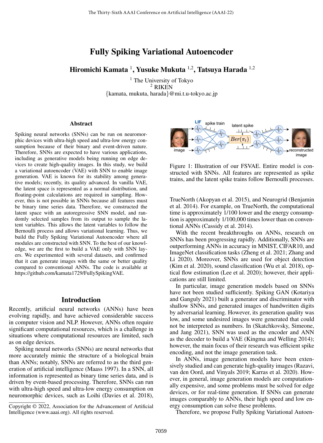
The Fully Spiking Variational Autoencoder (FSVAE) is an end-to-end spiking neural network (SNN) generative model designed to operate entirely with binary spike trains across all components. An input image $x$ is converted into binary spike trains $x_{1:T} \in \{0, 1\}^{C_{in} \times H \times W \times T}$ over $T$ discrete timesteps via direct input encoding.

The FSVAE architecture consists of:
1. SNN Encoder: A sequence of convolutional layers with kernel size $3$ and stride $2$ , threshold-dependent batch normalization (tdBN), and leaky integrate-and-fire (LIF) neurons that map $x_{1:T}$ into encoder spike features $x^E_{1:T} \in \{0, 1\}^{C \times T}$ , with latent channel dimensionality $C = 128$ .
2. Autoregressive Posterior SNN ( $f_q$ ): Formed by three fully connected layers that take the concatenated vector $(z_{q,t-1}, x^E_t) \in \{0, 1\}^{2C}$ (with $z_{q,0} = 0$ ) and output latent spikes $z_{q,t} \in \{0, 1\}^C$ sequentially for $t = 1, \dots, T$ .
3. Autoregressive Prior SNN ( $f_p$ ): Formed by three fully connected layers that take previous latent sample $z_{p,t-1} \in \{0, 1\}^C$ (with $z_{p,0} = 0$ ) and sequentially output prior latent spikes $z_{p,t} \in \{0, 1\}^C$ .
4. SNN Decoder: Deconvolutional layers with tdBN and LIF neurons that convert sampled latent spikes $z_{1:T} \in \{0, 1\}^{C \times T}$ into output spike trains $\hat{x}_{1:T} \in \{0, 1\}^{C_{out} \times H \times W \times T}$ .
5. Spike-to-Image Decoding Layer: A non-firing LIF neuron layer that converts the spike trains $\hat{x}_{1:T}$ into a continuous reconstructed image $\hat{x}$ using the final membrane potential.
Knowl 2 — Autoregressive Bernoulli Spike Sampling
model/method
In the Fully Spiking Variational Autoencoder (FSVAE), the latent space is modeled as a discrete Bernoulli process rather than a continuous Gaussian distribution to maintain full binary compatibility with neuromorphic hardware:

$q(z_{1:T} \mid x_{1:T}) = \prod_{t=1}^T q(z_t \mid x_{\le t}, z_{<t}) = \prod_{t=1}^T \text{Ber}(\pi_{q,t})$

$p(z_{1:T}) = \prod_{t=1}^T p(z_t \mid z_{<t}) = \prod_{t=1}^T \text{Ber}(\pi_{p,t})$

At each timestep $t \in \{1, \dots, T\}$ , autoregressive spiking networks $f_q$ and $f_p$ produce binary spike output vectors:

$\zeta_{q,t} := f_q(z_{q,t-1}, x^E_t; \Theta_{q,t}) \in \{0, 1\}^{kC}$

$\zeta_{p,t} := f_p(z_{p,t-1}; \Theta_{p,t}) \in \{0, 1\}^{kC}$

where $C$ is the latent dimension, $k \ge 2$ is an expansion integer factor (set to $k=20$ ), $x^E_t \in \{0, 1\}^C$ is the encoder spike output, and $\Theta_{q,t}, \Theta_{p,t}$ denote the membrane potentials of neurons in $f_q$ and $f_p$ .

Binary latent spikes $z_{\cdot, t, c} \in \{0, 1\}$ for each dimension $c \in \{1, \dots, C\}$ are generated by uniformly selecting one spike at random from the corresponding $k$ -element segment:

$z_{q,t,c} = \text{random\_select}(\zeta_{q,t}[k(c-1) : kc])$

$z_{p,t,c} = \text{random\_select}(\zeta_{p,t}[k(c-1) : kc])$

This sampling operation corresponds to drawing from Bernoulli distributions with parameters:

$\pi_{q,t,c} = \frac{1}{k} \sum_{j=k(c-1)}^{kc-1} \zeta_{q,t}[j]$

$\pi_{p,t,c} = \frac{1}{k} \sum_{j=k(c-1)}^{kc-1} \zeta_{p,t}[j]$
Knowl 3 — Spike-to-Image Decoding via Non-Firing Output Membrane Potential
equation
In the Fully Spiking Variational Autoencoder (FSVAE), the output layer converts reconstructed spike trains $\hat{x}_{1:T} \in \{0, 1\}^{C_{out} \times H \times W \times T}$ into a continuous reconstructed image $\hat{x} \in \mathbb{R}^{C_{out} \times H \times W}$ using non-firing leaky integrate-and-fire (LIF) neurons. The terminal membrane potential $u^{out}_T$ accumulates the output spikes over all $T$ timesteps according to:

$u^{out}_T = \sum_{t=1}^T \tau_{out}^{T-t} \hat{x}_t$

where $\tau_{out} = 0.8$ is the membrane potential decay factor. The continuous reconstructed image $\hat{x}$ is calculated by:

$\hat{x} = \tanh(u^{out}_T)$
Knowl 4 — Maximum Mean Discrepancy Loss with Postsynaptic Potential Kernel
equation
In the Fully Spiking Variational Autoencoder (FSVAE), the prior and posterior latent distributions are aligned using the Maximum Mean Discrepancy (MMD) with a postsynaptic potential (PSP) kernel function $k(z_{1:T}, z'_{1:T}) = \sum_{t=1}^T \text{PSP}(z_{\le t}) \text{PSP}(z'_{\le t})$ . The training objective function $\mathcal{L}$ is:

$\mathcal{L} = \text{MSE}(x, \hat{x}) + \sum_{t=1}^T \|\text{PSP}(\pi_{q, \le t}) - \text{PSP}(\pi_{p, \le t})\|^2$

where $\text{MSE}(x, \hat{x})$ is the mean squared error reconstruction loss between the input image $x$ and the decoded image $\hat{x}$ , and $\pi_{q,t}, \pi_{p,t} \in [0, 1]^C$ are the Bernoulli probability vectors of the posterior and prior at time $t$ . The first-order synaptic filter $\text{PSP}(v_{\le t})$ is computed iteratively for any time series $v_{1:T}$ via:

$\text{PSP}(v_{\le t}) = \left(1 - \frac{1}{\tau_{syn}}\right) \text{PSP}(v_{\le t-1}) + \frac{1}{\tau_{syn}} v_t$

with initial condition $\text{PSP}(v_{\le 0}) = 0$ , where $\tau_{syn}$ is the synaptic time constant.
Knowl 5 — FSVAE Training Protocol with Teacher Forcing and Scheduled Sampling
algorithm
The training routine for the Fully Spiking Variational Autoencoder uses teacher forcing and linear scheduled sampling to stabilize autoregressive latent recurrence and avoid posterior collapse.
Input: Dataset $D$ , total epochs $E = 150$ , batch size $B = 250$ , learning rate $\eta = 0.001$ , weight decay $\lambda = 0.001$ , timesteps $T = 16$ , channel expansion factor $k = 20$ .
Output: Trained FSVAE parameters.
Initialize encoder, prior $f_p$ , posterior $f_q$ , and decoder SNN parameters.
for epoch = 1 to $E$ do
     $\epsilon_{sched} \leftarrow 0.3 \times (\text{epoch} / E)$
    for each mini-batch $x \in D$ do
        Encode $x$ to spike train $x_{1:T}$ via direct input encoding.
        Pass $x_{1:T}$ through SNN encoder to obtain $x^E_{1:T}$ .
        Initialize $z_{q,0} \leftarrow 0$ , $z_{p,0} \leftarrow 0$ , $\text{PSP}_q \leftarrow 0$ , $\text{PSP}_p \leftarrow 0$ , $\mathcal{L}_{MMD} \leftarrow 0$ .
        for $t = 1$ to $T$ do
            Compute posterior output $\zeta_{q,t} = f_q(z_{q,t-1}, x^E_t) \in \{0, 1\}^{kC}$ .
            Compute $\pi_{q,t,c} = \text{mean}(\zeta_{q,t}[k(c-1):kc])$ for $c \in \{1, \dots, C\}$ .
            Sample $z_{q,t,c} = \text{random\_select}(\zeta_{q,t}[k(c-1):kc])$ .
            Sample $r \sim \text{Uniform}(0, 1)$ .
            if $r < \epsilon_{sched}$ then
                 $z_{in, t-1} \leftarrow z_{p,t-1}$
            else
                 $z_{in, t-1} \leftarrow z_{q,t-1}$
            Compute prior output $\zeta_{p,t} = f_p(z_{in, t-1}) \in \{0, 1\}^{kC}$ .
            Compute $\pi_{p,t,c} = \text{mean}(\zeta_{p,t}[k(c-1):kc])$ for $c \in \{1, \dots, C\}$ .
            Sample $z_{p,t,c} = \text{random\_select}(\zeta_{p,t}[k(c-1):kc])$ .
            Update $\text{PSP}_q \leftarrow (1 - 1/\tau_{syn})\text{PSP}_q + (1/\tau_{syn})\pi_{q,t}$ .
            Update $\text{PSP}_p \leftarrow (1 - 1/\tau_{syn})\text{PSP}_p + (1/\tau_{syn})\pi_{p,t}$ .
             $\mathcal{L}_{MMD} \leftarrow \mathcal{L}_{MMD} + \|\text{PSP}_q - \text{PSP}_p\|^2$ .
        Pass $z_{q,1:T}$ through SNN decoder to obtain $\hat{x}_{1:T}$ .
        Compute reconstructed image $\hat{x} = \tanh(\sum_{t=1}^T \tau_{out}^{T-t} \hat{x}_t)$ .
         $\mathcal{L} \leftarrow \text{MSE}(x, \hat{x}) + \mathcal{L}_{MMD}$ .
        Backpropagate $\mathcal{L}$ using surrogate gradient $\frac{\partial o}{\partial u} = \frac{1}{a} \text{sign}(|u - V_{th}| < a/2)$ .
        Update parameters using AdamW.

Knowl 6 — Image Generation Performance Benchmark across Datasets

data/table

Performance comparison between a standard continuous ANN VAE and the proposed Fully Spiking Variational Autoencoder (FSVAE) on MNIST ( $32\times 32$ ), FashionMNIST ( $32\times 32$ ), CIFAR10 ( $32\times 32$ ), and CelebA ( $64\times 64$ ). Evaluated metrics include Mean Squared Error Reconstruction Loss, Inception Score (IS), Fréchet Inception Distance (Inception FID), and Fréchet Distance measured on the latent space of a pretrained dataset-specific Autoencoder (Autoencoder FID) over 5,000 generated samples.

Dataset	Model	Reconstruction Loss $\downarrow$	Inception Score $\uparrow$	Inception FID $\downarrow$	Autoencoder FID $\downarrow$
MNIST	ANN	0.048	5.947	112.5	17.09
MNIST	FSVAE (Ours)	0.031	6.209	97.06	35.54
FashionMNIST	ANN	0.050	4.252	123.7	18.08
FashionMNIST	FSVAE (Ours)	0.031	4.551	90.12	15.75
CIFAR10	ANN	0.105	2.591	229.6	196.9
CIFAR10	FSVAE (Ours)	0.066	2.945	175.5	133.9
CelebA	ANN	0.059	3.231	92.53	156.9
CelebA	FSVAE (Ours)	0.051	3.697	101.6	112.9

FSVAE achieves lower reconstruction errors and higher Inception Scores across all four datasets compared to the ANN VAE baseline. For FashionMNIST and CIFAR10, FSVAE outperforms the ANN VAE across all four evaluation metrics.

Knowl 7 — Inference Computational Complexity Comparison

data/table

Computational complexity measured in floating-point addition and multiplication operations required to perform inference on a single MNIST image ( $32\times 32$ ) with $T=16$ timesteps:

FSVAE requires 6.8 times more additions than the ANN VAE due to temporal unrolling across 16 timesteps, but reduces the number of multiplications by a factor of 13.2 (a $14.8\times$ reduction in the spiking layers). Because multiplication requires significantly more power and circuit area than addition in neuromorphic hardware, this shift reduces overall energy consumption.

Knowl 8 — Ablation on Latent Distance Metric and PSP Filtering
empirical result
In an ablation study on the CelebA dataset ( $64\times 64$ ), the effect of different latent distribution alignment objectives in the ELBO loss function was evaluated using Fréchet Inception Distance (FID):
- Kullback-Leibler Divergence (KLD) (with $\epsilon = 0.01$ added to $\pi_{q,t}$ and $\pi_{p,t}$ to prevent numerical divergence): FID $= 114.3$ .
- Maximum Mean Discrepancy (MMD) without postsynaptic potential filtering: FID $= 106.0$ .
- Maximum Mean Discrepancy (MMD) with PSP Kernel: FID $= 101.6$ .
The combination of MMD and postsynaptic potential (PSP) filtering yielded the lowest FID score, confirming that temporal synaptic filtering effectively captures spike train dynamics while avoiding the divergence and runaway self-excitation issues of KL divergence.
Knowl 9 — Sensitivity of FSVAE Generation to Timestep Count and Channel Multiplier
empirical result
On the MNIST dataset, the sample generation quality (measured by FID) of the Fully Spiking Variational Autoencoder varies with the number of timesteps $T$ and channel multiplier $k$ :
- Timestep count $T$ : Evaluated across $T \in [4, 24]$ , FID reaches an optimal minimum at $T = 16$ (FID $\approx 97.06$ , compared to the ANN VAE baseline of $112.5$ ). Fewer timesteps ( $T < 16$ ) lack expressive capacity, whereas larger values ( $T > 16$ ) enlarge the latent space excessively, causing generation quality to degrade.
- Channel expansion factor $k$ : Evaluated across $k \in [5, 30]$ , FID consistently outperforms the ANN VAE baseline across all tested values of $k$ , with the best generation FID achieved at $k = 20$ .

Coverage note — None omitted; all core contributions, including the FSVAE architecture, autoregressive Bernoulli spike sampling, membrane-potential decoding, PSP-MMD loss formulation, training algorithms, and benchmark experiments have been fully covered.

Citation

MLA

Kamata, H., et al. “Fully Spiking Variational Autoencoder”. arXiv, 2021, http://arxiv.org/abs/2110.00375v3.

APA

Kamata, H., Mukuta, Y., & Harada, T. (2021). Fully Spiking Variational Autoencoder. arXiv. http://arxiv.org/abs/2110.00375v3

Chicago

Kamata, H., Y. Mukuta, and T. Harada. 2021. “Fully Spiking Variational Autoencoder”. arXiv. http://arxiv.org/abs/2110.00375v3.

Harvard

Kamata, H., Mukuta, Y. and Harada, T. (2021) “Fully Spiking Variational Autoencoder”, arXiv [Preprint]. Available at: http://arxiv.org/abs/2110.00375v3.

Vancouver

1. Kamata H, Mukuta Y, Harada T (2021) Fully Spiking Variational Autoencoder. arXiv

BibTeX

@article{kamata2021fully,
  title = {Fully Spiking Variational Autoencoder},
  author = {Kamata, Hiromichi and Mukuta, Yusuke and Harada, Tatsuya},
  year = {2021},
  journal = {arXiv},
  url = {http://arxiv.org/abs/2110.00375v3},
  eprint = {2110.00375}
}

Metadata:arXiv

Access the Paper

This paper is available from its original source. Click below to access the PDF.

Open PDF

Model	Addition	Multiplication
ANN	$7.4 \times 10^9$	$7.4 \times 10^9$
FSVAE (Ours)	$5.0 \times 10^{10}$	$5.6 \times 10^8$

Fully Spiking Variational Autoencoder

Abstract

Topics

Keywords

Table of Contents

Knowls

Knowl 1 — Fully Spiking Variational Autoencoder Architecture

Knowl 2 — Autoregressive Bernoulli Spike Sampling

Knowl 3 — Spike-to-Image Decoding via Non-Firing Output Membrane Potential

Knowl 4 — Maximum Mean Discrepancy Loss with Postsynaptic Potential Kernel

Knowl 5 — FSVAE Training Protocol with Teacher Forcing and Scheduled Sampling

Knowl 6 — Image Generation Performance Benchmark across Datasets

Knowl 7 — Inference Computational Complexity Comparison

Knowl 8 — Ablation on Latent Distance Metric and PSP Filtering

Knowl 9 — Sensitivity of FSVAE Generation to Timestep Count and Channel Multiplier

Citation

BibTeX

Access the Paper