Decompose, Adjust, Compose: Effective Normalization by Playing with Frequency for Domain Generalization

Sangrok LeeJongseong BaeHa Young Kim

article2023CVPR68 citations

Proposes a frequency-domain normalization framework that separates and regulates amplitude and phase variations to eliminate domain-specific styles while preserving essential semantic content for domain generalization.

Listen

Deep learning models frequently suffer significant performance degradation when deployed on unseen data distributions, a major operational risk for computer vision applications. To build models that remain robust across different environments, researchers rely on domain generalization. Standard approaches often use feature normalization to strip away domain-specific style information, treating statistical measures as style and normalized features as content. However, this process unintentionally distorts the core content information, undermining the model's reliability.

The article aims to explain and resolve this content distortion by analyzing normalization through frequency analysis and introducing feature-level normalization techniques that systematically regulate content and style variations for robust computer vision models.

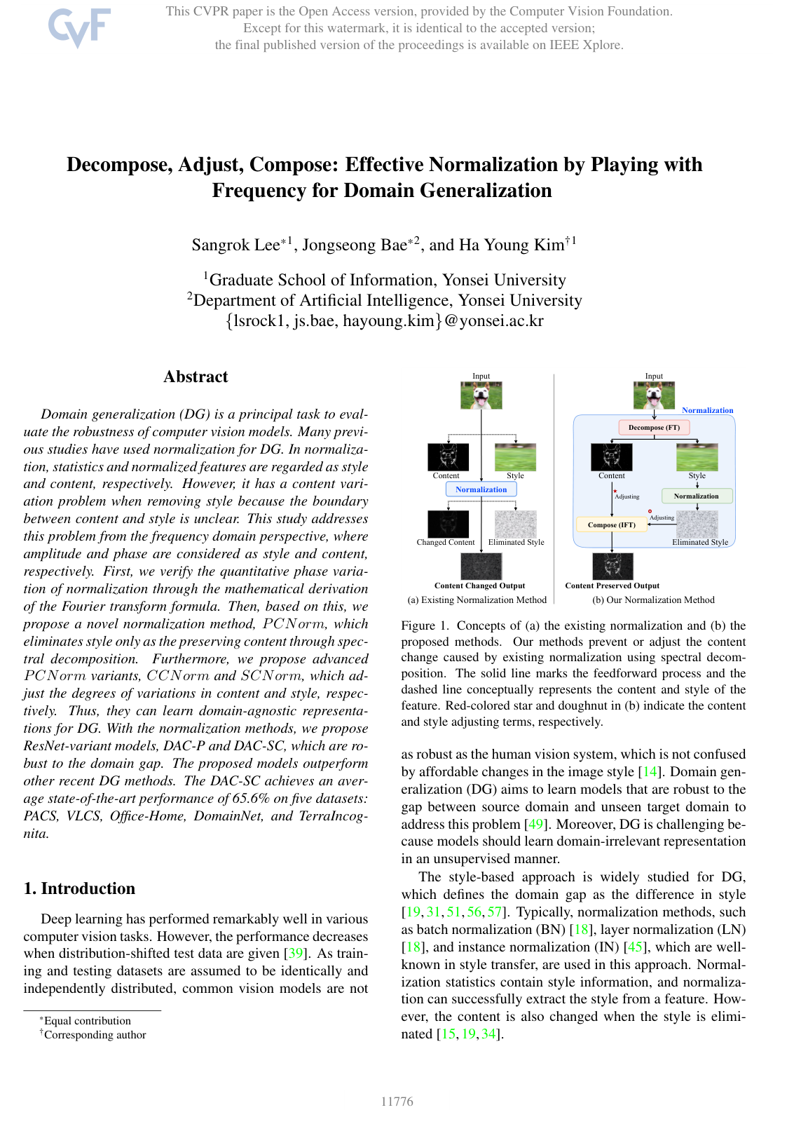
The researchers mathematically demonstrated using the Fourier transform that the statistical mean shift in traditional normalization directly causes phase distortion, which alters the underlying image content. Based on this finding, they developed Phase-Consistent Normalization (PCNorm), which preserves original content by recombining the phase of pre-normalized features with the amplitude (style) of post-normalized features. They further expanded this concept into Content-Controlling Normalization (CCNorm) and Style-Controlling Normalization (SCNorm), which use learnable parameters to adjust the exact balance between original and normalized content and style. These modules were integrated into standard ResNet architectures to create two specialized models, DAC-P and DAC-SC, and evaluated across five major domain generalization benchmark datasets spanning thousands of multi-domain images: VLCS, PACS, Office-Home, DomainNet, and TerraIncognita.

The evaluation produced several key findings: First, the primary model, DAC-SC, established a new benchmark by achieving an average accuracy of 65.6% across all five datasets, outperforming established baseline methods. Second, DAC-SC achieved top performances on individual benchmarks, including 87.5% on PACS, 70.3% on Office-Home, and 44.9% on DomainNet (a 3.7 percentage point increase over the standard baseline). Third, controlling content and style through learnable parameters (CCNorm and SCNorm) generally provided superior generalization over strict content preservation (PCNorm). Fourth, in datasets with minimal domain shift like TerraIncognita, preserving pure content via PCNorm proved more effective (49.8% accuracy) than active adjustment.

These findings indicate that completely eliminating style or rigidly freezing content is suboptimal for real-world robustness. Instead, allowing vision models to learn the appropriate degree of content preservation and style filtering at intermediate network stages significantly improves out-of-distribution accuracy. For organizations deploying vision systems in uncontrolled environments, adopting these normalization techniques reduces operational failure risks and improves model reliability without needing target domain retraining.

Organizations developing computer vision pipelines should consider replacing standard normalization in downsampling and transition layers with content- and style-controlling modules. For tasks with severe domain gaps, DAC-SC is recommended, whereas applications with minor domain variations should favor the simpler PCNorm approach. Future work should evaluate these frequency-based normalization layers across different neural architectures beyond ResNet and in broader vision tasks.

The results carry high confidence based on consistent multi-trial evaluations across standard industry benchmarks. However, stakeholders should note that the empirical validations were primarily conducted using ResNet backbones in image classification settings, and adjustments may be needed when transferring the approach to other model families or complex multimodal tasks.

arXiv: 2303.02328

No sufficiently relevant recommendations were found.
Cover for Decompose, Adjust, Compose: Effective Normalization by Playing with Frequency for Domain Generalization

Table of Contents

  • 1. Introduction
  • 2. Related Work
  • 3. Analysis
  • 3.1. Spectral Decomposition
  • 3.2. Content Variation by Normalization
  • 4. Proposed Method
  • 4.1. Phase Consistent Normalization (PCNorm)
  • 4.2. Content Controlling Normalization (CCNorm)
  • 4.3. Style Controlling Normalization (SCNorm)
  • 4.4. DAC-P and DAC-SC
  • 5. Experiment
  • 5.1. Dataset
  • 5.2. Experimental Details
  • 5.3. Comparison with SOTA Methods
  • 5.4. Ablation Study
  • 6. Conclusion
  • 7. Acknowledgement
  • References

Knowls

  1. Knowl 1 — Mathematical Formulation of Content Distortion via Normalization Phase Shift

    theoretical result

    Spatial feature normalization alters the underlying content information of a feature map by introducing a phase shift in the frequency domain, where content is represented by phase and style is represented by amplitude.

    Let a 2D spatial feature map be f∈Rh×wf \in \mathbb{R}^{h \times w}, whose Discrete Fourier Transform (DFT) is given by:

    F(u,v)=1wh∑x=0w−1∑y=0h−1f(x,y)exp⁡(i2π(uxw+vyh))=Freal(u,v)+i Fimg(u,v)\mathcal{F}(u,v) = \frac{1}{wh}\sum_{x=0}^{w-1}\sum_{y=0}^{h-1} f(x,y)\exp\left(i 2\pi \left(\frac{ux}{w}+\frac{vy}{h}\right)\right) = \mathcal{F}_{\text{real}}(u,v) + i \,\mathcal{F}_{\text{img}}(u,v)

    with amplitude α=Freal2+Fimg2\alpha = \sqrt{\mathcal{F}_{\text{real}}^2 + \mathcal{F}_{\text{img}}^2} and phase ρ=arctan⁡(FimgFreal)\rho = \arctan\left(\frac{\mathcal{F}_{\text{img}}}{\mathcal{F}_{\text{real}}}\right).

    When ff is normalized to fnorm=f−μσf^{\text{norm}} = \frac{f - \mu}{\sigma} with statistical mean μ\mu and standard deviation σ\sigma, the frequency components of fnormf^{\text{norm}} relate to the original Fourier components by:

    Frealnorm=Freal−Frealμσ,Fimgnorm=Fimg−Fimgμσ\mathcal{F}_{\text{real}}^{\text{norm}} = \frac{\mathcal{F}_{\text{real}} - \mathcal{F}_{\text{real}}^{\mu}}{\sigma}, \quad \mathcal{F}_{\text{img}}^{\text{norm}} = \frac{\mathcal{F}_{\text{img}} - \mathcal{F}_{\text{img}}^{\mu}}{\sigma}

    where Frealμ\mathcal{F}_{\text{real}}^{\mu} and Fimgμ\mathcal{F}_{\text{img}}^{\mu} are the Fourier components of a constant feature map fμ∈Rh×wf^{\mu} \in \mathbb{R}^{h \times w} whose entries all equal μ\mu.

    The amplitude αnorm\alpha^{\text{norm}} and phase ρnorm\rho^{\text{norm}} of the normalized feature fnormf^{\text{norm}} are:

    αnorm=(Freal−Frealμ)2+(Fimg−Fimgμ)2σ\alpha^{\text{norm}} = \frac{\sqrt{(\mathcal{F}_{\text{real}} - \mathcal{F}_{\text{real}}^{\mu})^2 + (\mathcal{F}_{\text{img}} - \mathcal{F}_{\text{img}}^{\mu})^2}}{\sigma}

    ρnorm=arctan⁡(Fimg−FimgμFreal−Frealμ)\rho^{\text{norm}} = \arctan\left(\frac{\mathcal{F}_{\text{img}} - \mathcal{F}_{\text{img}}^{\mu}}{\mathcal{F}_{\text{real}} - \mathcal{F}_{\text{real}}^{\mu}}\right)

    Because σ\sigma cancels out in ρnorm\rho^{\text{norm}}, the shift between original phase ρ\rho and normalized phase ρnorm\rho^{\text{norm}} is entirely governed by the spatial mean shift μ\mu. The degree of content distortion increases monotonically with the magnitude of μ\mu.

  2. Knowl 2 — Phase-Consistent Normalization (PCNorm)

    model/method

    Phase-Consistent Normalization (PCNorm) is a feature normalization module that removes domain-specific style while preserving the original content of the input feature map by recombining the phase of the pre-normalized feature with the amplitude of the post-normalized feature.

    Given an input spatial feature f∈Rh×wf \in \mathbb{R}^{h \times w}, Batch Normalization (BN) is applied to compute fnorm=BatchNorm(f)f^{\text{norm}} = \text{BatchNorm}(f). Both ff and fnormf^{\text{norm}} are mapped to the frequency domain via Discrete Fourier Transform (DFT), decomposed into (α,ρ)(\alpha, \rho) and (αnorm,ρnorm)(\alpha^{\text{norm}}, \rho^{\text{norm}}), respectively, where α\alpha denotes amplitude and ρ\rho denotes phase.

    PCNorm synthesizes a content-invariant normalized feature map using the Inverse Discrete Fourier Transform (IFT):

    PCNorm(f)=IFT(compose(αnorm,ρ))\text{PCNorm}(f) = \text{IFT}(\text{compose}(\alpha^{\text{norm}}, \rho))

    where compose(α,ρ)=αcos⁡(ρ)+i αsin⁡(ρ)\text{compose}(\alpha, \rho) = \alpha \cos(\rho) + i\,\alpha \sin(\rho). By discarding ρnorm\rho^{\text{norm}} and retaining ρ\rho, PCNorm eliminates the content degradation caused by the mean shift μ\mu during normalization.

  3. Knowl 3 — Content-Controlling Normalization (CCNorm)

    model/method

    Content-Controlling Normalization (CCNorm) is an adaptive normalization module that regulates the degree of content variation during normalization instead of completely preserving the pre-normalized phase.

    Given an input feature f∈Rh×wf \in \mathbb{R}^{h \times w}, its mean μ\mu, a learnable parameter vector λc∈R2\lambda^c \in \mathbb{R}^2, and a temperature hyperparameter TcT_c, the content-adjusting weights are computed via softmax:

    (λnormc,λorgc)=softmax(λcTc)(\lambda^c_{\text{norm}}, \lambda^c_{\text{org}}) = \text{softmax}\left(\frac{\lambda^c}{T_c}\right)

    A content-adjusted spatial feature fcf^c is defined as:

    fc=f−μλnormcf^c = f - \mu \lambda^c_{\text{norm}}

    Applying the Discrete Fourier Transform (DFT) to fcf^c yields the modulated phase ρc\rho^c. The post-normalized amplitude αnorm\alpha^{\text{norm}} is extracted via DFT from fnorm=BatchNorm(f)f^{\text{norm}} = \text{BatchNorm}(f). CCNorm composes the normalized amplitude with the adjusted phase:

    CCNorm(f)=IFT(compose(αnorm,ρc))\text{CCNorm}(f) = \text{IFT}(\text{compose}(\alpha^{\text{norm}}, \rho^c))

    When λnormc=0\lambda^c_{\text{norm}} = 0, ρc=ρ\rho^c = \rho (full content preservation); when λnormc=1\lambda^c_{\text{norm}} = 1, ρc=ρnorm\rho^c = \rho^{\text{norm}} (standard normalization).

  4. Knowl 4 — Style-Controlling Normalization (SCNorm)

    model/method

    Style-Controlling Normalization (SCNorm) is an adaptive normalization module that controls the degree of style elimination by blending the original feature amplitude with the normalized feature amplitude while preserving content phase.

    Given an input feature f∈Rh×wf \in \mathbb{R}^{h \times w}, standard Instance Normalization (IN) produces fnorm=InstanceNorm(f)f^{\text{norm}} = \text{InstanceNorm}(f). The input ff is decomposed via Discrete Fourier Transform (DFT) into amplitude α\alpha and phase ρ\rho, and fnormf^{\text{norm}} is decomposed into amplitude αnorm\alpha^{\text{norm}} and phase ρnorm\rho^{\text{norm}}.

    With a learnable parameter vector λs∈R2\lambda^s \in \mathbb{R}^2 and temperature hyperparameter TsT_s, the style-adjusting weights are computed as:

    (λnorms,λorgs)=softmax(λsTs)(\lambda^s_{\text{norm}}, \lambda^s_{\text{org}}) = \text{softmax}\left(\frac{\lambda^s}{T_s}\right)

    SCNorm combines the scaled amplitudes with the original phase ρ\rho via Inverse Discrete Fourier Transform (IFT):

    SCNorm(f)=IFT(compose(λnormsαnorm+λorgsα,ρ))\text{SCNorm}(f) = \text{IFT}(\text{compose}(\lambda^s_{\text{norm}} \alpha^{\text{norm}} + \lambda^s_{\text{org}} \alpha, \rho))

    When λnorms=0\lambda^s_{\text{norm}} = 0, SCNorm acts as an identity function on amplitude, preserving the original style α\alpha. When λnorms=1\lambda^s_{\text{norm}} = 1, SCNorm completely removes the style via IN.

  5. Knowl 5 — Algorithms for PCNorm, CCNorm, and SCNorm

    algorithm

    The frequency-domain normalization methods PCNorm, CCNorm, and SCNorm operate on spatial feature maps ff using standard Fourier decomposition and composition routines.

    def pcnorm(f):
        f_norm = batch_norm(f)
        F = FT(f)
        F_norm = FT(f_norm)
        a, p = decompose(F)
        a_norm, p_norm = decompose(F_norm)
        f_out = IFT(compose(a_norm, p))
        return f_out
    
    def ccnorm(f, weight, T_c, mean):
        weight_c = softmax(weight / T_c, dim=0)
        fc = f - mean * weight_c[0]
        f_norm = batch_norm(f)
        FC = FT(fc)
        F_norm = FT(f_norm)
        ac, pc = decompose(FC)
        a_norm, p_norm = decompose(F_norm)
        f_out = IFT(compose(a_norm, pc))
        return f_out
    
    def scnorm(f, weight, T_s):
        weight_s = softmax(weight / T_s, dim=0)
        f_norm = instance_norm(f)
        F = FT(f)
        F_norm = FT(f_norm)
        a, p = decompose(F)
        a_norm, p_norm = decompose(F_norm)
        f_out = IFT(compose(a_norm * weight_s[0] + a * weight_s[1], p))
        return f_out
    

    Here, FT and IFT denote 2D discrete Fourier transform and its inverse. decompose converts complex frequency features to amplitude and phase, and compose converts amplitude and phase back into complex frequency features. In ccnorm, mean is the batch mean during training and the running cumulative mean during testing. In DAC-SC, the learnable parameters weight are initialized to 0, and temperatures are set to Tc=10−6T_c = 10^{-6} and Ts=10−1T_s = 10^{-1}.

  6. Knowl 6 — DAC-P and DAC-SC ResNet Architectures

    model/method

    DAC-P and DAC-SC are domain generalization architectures built upon the ResNet-50 backbone by strategically integrating frequency-domain normalizations into downsampling layers and residual block stages.

    In standard ResNet residual blocks (H(x)+xH(x) + x), the downsampling skip path uses a 1×11 \times 1 convolution with stride 2 followed by Batch Normalization (BN):

    downsample(x)=BatchNorm(Conv(x))\text{downsample}(x) = \text{BatchNorm}(\text{Conv}(x))

    Because spatial resizing alters the phase and BN introduces content shift via its mean shift μ\mu, downsampling layers suffer from aggravated content distortion.

    1. DAC-P: Replaces the BN in all four downsampling layers of ResNet-50 with PCNorm:

    downsamplep(x)=PCNorm(Conv(x))\text{downsample}_p(x) = \text{PCNorm}(\text{Conv}(x))

    1. DAC-SC: Uses CCNorm in place of BN in all four downsampling layers:

    downsamplec(x)=CCNorm(Conv(x))\text{downsample}_c(x) = \text{CCNorm}(\text{Conv}(x))

    Additionally, DAC-SC inserts SCNorm modules as style regularizers at the ends of Stage 1, Stage 2, and Stage 3 of ResNet-50. Learnable parameters λc\lambda^c and λs\lambda^s are initialized to 00, with temperatures Tc=10−6T_c = 10^{-6} and Ts=10−1T_s = 10^{-1}. The affine transform parameters of base normalizations are applied at the output of the respective normalization layers.

  7. Knowl 7 — Domain Generalization Performance Comparison on Standard Benchmarks

    data/table

    The performance of DAC-P and DAC-SC was evaluated against standard DG baselines and recent state-of-the-art methods across five benchmark datasets using a ResNet-50 backbone following the DomainBed protocol (evaluating out-of-domain test accuracy with training-domain validation selection).

    Model VLCS PACS Office-Home DomainNet TerraIncognita Avg
    ERM 77.4 0.3 85.7 0.5 67.5 0.5 41.2 0.2 47.2 0.4 63.8
    IRM 78.5 0.5 83.5 0.8 64.3 2.2 33.9 2.8 47.6 0.8 61.6
    GroupDRO 76.7 0.6 84.4 0.8 66.0 0.7 33.3 0.2 43.2 1.1 60.7
    Mixup 77.4 0.6 84.6 0.6 68.1 0.3 39.2 0.1 47.9 0.8 63.4
    MLDG 77.2 0.4 84.9 1.0 66.8 0.6 41.2 0.1 47.7 0.9 63.6
    CORAL 78.8 0.6 86.2 0.3 68.7 0.3 41.5 0.1 47.6 1.0 64.5
    MMD 77.5 0.9 84.6 0.5 66.3 0.1 23.4 9.5 42.2 1.6 58.8
    DANN 78.6 0.4 83.6 0.4 65.9 0.6 38.3 0.1 46.7 0.5 62.6
    CDANN 77.5 0.1 82.6 0.9 65.8 1.3 38.3 0.3 45.8 1.6 62.0
    MTL 77.2 0.4 84.6 0.5 66.4 0.5 40.6 0.1 45.6 1.2 62.9
    ARM 77.6 0.3 85.1 0.4 64.8 0.3 35.5 0.2 45.5 0.3 61.7
    VREx 78.3 0.2 84.9 0.6 66.4 0.6 33.6 2.9 46.4 0.6 61.9
    RSC 77.1 0.5 85.2 0.9 65.5 0.9 38.9 0.5 46.6 1.0 62.7
    IIB 77.2 1.6 83.9 0.2 68.6 0.1 41.5 2.3 45.8 1.4 63.4
    SelfReg 77.8 0.9 85.6 0.4 67.9 0.7 42.8 0.0 47.0 0.3 64.2
    SagNet 77.8 0.5 86.3 0.2 68.1 0.1 40.3 0.1 48.6 1.0 64.2
    DAC-P 77.0 0.6 85.6 0.5 69.5 0.1 43.8 0.3 49.8 0.2 65.1
    DAC-SC 78.7 0.3 87.5 0.1 70.3 0.2 44.9 0.1 46.5 0.3 65.6

    DAC-SC achieves the highest average accuracy across all five datasets (65.6%), establishing new state-of-the-art results on PACS (87.5%), Office-Home (70.3%), and DomainNet (44.9%). On TerraIncognita, where domain distribution shifts are smaller due to fixed camera trap locations, DAC-P achieves the top accuracy of 49.8%.

  8. Knowl 8 — Ablation on Component Positions and Combinations in DAC Architectures

    data/table

    An ablation study evaluated the placement and combinations of PCNorm, CCNorm, and SCNorm within a ResNet-50 architecture. Module positions are designated as Downsample layer (D) or End of stage (E).

    Row Method Position VLCS PACS Office-Home DomainNet TerraIncognita Avg
    1 ResNet (Baseline) - 77.4 85.7 67.5 41.2 47.2 63.8
    2 + CCNorm D 77.1 86.0 69.9 44.7 48.1 65.1 (+1.3)
    3 + SCNorm E 78.7 87.4 70.3 44.9 46.5 65.6 (+0.5)
    4 + PCNorm D 77.0 85.6 69.5 43.8 49.8 65.1 (+1.3)
    5 + SCNorm E 77.1 86.0 68.8 44.6 48.0 64.9 (-0.2)
    6 + SCNorm D 77.3 86.4 69.2 44.5 45.3 64.5 (+0.7)
    7 + SCNorm E 77.3 86.8 69.2 44.9 43.0 64.3 (-0.2)

    Key observations:

    1. Adding CCNorm to the downsample layers (Row 2) improves average accuracy by +1.3% over the ResNet baseline. Adding SCNorm at stage ends (Row 3, DAC-SC) provides an additional +0.5% gain, reaching 65.6%.
    2. Although PCNorm and CCNorm achieve the same 65.1% average when used alone in downsample layers, CCNorm outperforms PCNorm on 4 out of 5 datasets (all except TerraIncognita).
    3. Combining SCNorm with PCNorm (Row 5) leads to a -0.2% degradation, showing that SCNorm is synergistic specifically with CCNorm.
    4. Placing SCNorm in downsample layers (Row 6) achieves only +0.7% improvement, confirming that regulating content change (CCNorm/PCNorm) is the appropriate mechanism for downsampling layers.
  9. Knowl 9 — Ablation on Base Normalization Type for SCNorm

    data/table

    An ablation study evaluated the choice of base normalization used to compute fnormf^{\text{norm}} in SCNorm, comparing standard Instance Normalization (InNorm) against SCNorm implemented with Instance Normalization (SCNormin\text{SCNorm}_{\text{in}}), Layer Normalization (SCNormln\text{SCNorm}_{\text{ln}}), and Batch Normalization (SCNormbn\text{SCNorm}_{\text{bn}}).

    Method VLCS PACS Office-Home DomainNet TerraIncognita Avg
    InNorm 76.0 87.2 65.6 44.0 42.7 63.1
    SCNormin\text{SCNorm}_{\text{in}} 78.7 87.4 70.3 44.9 46.5 65.6
    SCNormln\text{SCNorm}_{\text{ln}} 75.0 87.3 67.9 44.3 44.3 63.8
    SCNormbn\text{SCNorm}_{\text{bn}} 77.0 86.6 70.3 44.8 46.9 65.1

    SCNormin\text{SCNorm}_{\text{in}} outperforms raw InNorm across all five datasets (improving average accuracy from 63.1% to 65.6%). Instance Normalization achieves the highest overall average performance among the normalization candidates for SCNorm, while Layer Normalization consistently performs worst (63.8% average).

  10. Knowl 10 — Stage-Wise Style Control Dynamics in SCNorm

    empirical result

    Analysis of the learned style-mixing parameters (λnorms,λorgs)(\lambda^s_{\text{norm}}, \lambda^s_{\text{org}}) across network depth reveals distinct functional roles for SCNorm at different stages:

    1. In early stages (SCNorm1 at the end of Stage 1 and SCNorm2 at the end of Stage 2), the learned original style weight λorgs\lambda^s_{\text{org}} varies across datasets but generally remains above 0.5.
    2. In deep features (SCNorm3 at the end of Stage 3), λorgs\lambda^s_{\text{org}} converges to an average of 0.98980.9898 across all five datasets, indicating that the original style amplitude α\alpha is almost completely preserved near the network output.
    3. Clamping λorgs=1.0\lambda^s_{\text{org}} = 1.0 permanently at SCNorm3 (eliminating style normalization entirely at Stage 3) causes average accuracy across all five datasets to drop from 65.6% to 64.5%, with individual drops exceeding 1.0% on VLCS (78.7% to 76.6%), Office-Home (70.3% to 69.3%), and TerraIncognita (46.5% to 44.9%). Even marginal adjustments to style elimination in deep layers are critical for generalization performance.

Coverage note — None was omitted; all novel theoretical derivations, proposed normalization methods, algorithms, network architectures, benchmark comparisons, and ablation analyses are covered.

References

  1. 1.Martin Arjovsky, Leon Bottou, Ishaan Gulrajani, and David Lopez-Paz. Invariant risk minimization. arXiv preprint arXiv:1907.02893, 2019. 7
  2. 2.Sara Beery, Grant Van Horn, and Pietro Perona. Recognition in terra incognita. ArXiv, abs/1807.04975, 2018. 6
  3. 3.Gilles Blanchard, Aniket Anand Deshmukh, Urun Dogan, Gyemin Lee, and Clayton D. Scott. Domain generalization by marginal transfer learning. J. Mach. Learn. Res., 22:2:1– 2:55, 2021. 3, 7
  4. 4.Ronald Newbold Bracewell and Ronald N Bracewell. The Fourier transform and its applications, volume 31999. McGraw-Hill New York, 1986. 2
  5. 5.John P Castagna and Shengjie Sun. Comparison of spectral decomposition methods. First break, 24(3), 2006. 3
  6. 6.Chaoqi Chen, Jiongcheng Li, Xiaoguang Han, Xiaoqing Liu, and Yizhou Yu. Compound domain generalization via meta- knowledge encoding. 2022 IEEE/CVF Conference on Com- puter Vision and Pattern Recognition (CVPR), pages 7109– 7119, 2022. 3
  7. 7.Guangyao Chen, Peixi Peng, Li Ma, Jia Li, Lin Du, and Yonghong Tian. Amplitude-phase recombination: Rethink- ing robustness of convolutional neural networks in frequency domain. 2021 IEEE/CVF International Conference on Com- puter Vision (ICCV), pages 448–457, 2021. 2
  8. 8.Jia Deng, Wei Dong, Richard Socher, Li-Jia Li, Kai Li, and Li Fei-Fei. Imagenet: A large-scale hierarchical image database. In 2009 IEEE conference on computer vision and pattern recognition, pages 248–255. Ieee, 2009. 6
  9. 9.Xinjie Fan, Qifei Wang, Junjie Ke, Feng Yang, Boqing Gong, and Mingyuan Zhou. Adversarially adaptive normal- ization for single domain generalization. In Proceedings of the IEEE/CVF Conference on Computer Vision and Pattern Recognition, pages 8208–8217, 2021. 2, 3
  10. 10.Yaroslav Ganin, E. Ustinova, Hana Ajakan, Pascal Germain, H. Larochelle, Francois Laviolette, Mario Marchand, and Victor S. Lempitsky. Domain-adversarial training of neural networks. In J. Mach. Learn. Res., 2016. 2, 7
  11. 11.Ishaan Gulrajani and David Lopez-Paz. In search of lost do- main generalization. ArXiv, abs/2007.01434, 2021. 7
  12. 12.Bruce C Hansen and Robert F Hess. Structural sparseness and spatial phase alignment in natural scenes. JOSA A, 24(7):1873–1885, 2007. 3
  13. 13.Kaiming He, X. Zhang, Shaoqing Ren, and Jian Sun. Deep residual learning for image recognition. 2016 IEEE Confer- ence on Computer Vision and Pattern Recognition (CVPR), pages 770–778, 2016. 2, 4, 6
  14. 14.Dan Hendrycks and Thomas G. Dietterich. Benchmarking neural network robustness to common corruptions and per- turbations. ArXiv, abs/1903.12261, 2019. 1
  15. 15.Xun Huang and Serge J. Belongie. Arbitrary style transfer in real-time with adaptive instance normalization. 2017 IEEE International Conference on Computer Vision (ICCV), pages 1510–1519, 2017. 1, 2, 3
  16. 16.Zeyi Huang, Haohan Wang, Eric P. Xing, and Dong Huang. Self-challenging improves cross-domain generalization. In ECCV, 2020. 2, 7
  17. 17.Eleftherios Ioannou and Steve Maddock. Depth-aware neu- ral style transfer using instance normalization. arXiv preprint arXiv:2203.09242, 2022. 3
  18. 18.Sergey Ioffe and Christian Szegedy. Batch normalization: Accelerating deep network training by reducing internal co- variate shift. ArXiv, abs/1502.03167, 2015. 1
  19. 19.Xin Jin, Cuiling Lan, Wenjun Zeng, Zhibo Chen, and Li Zhang. Style normalization and restitution for generaliz- able person re-identification. 2020 IEEE/CVF Conference on Computer Vision and Pattern Recognition (CVPR), pages 3140–3149, 2020. 1, 3, 5, 6
  20. 20.Daehee Kim, Youngjun Yoo, Seunghyun Park, Jinkyu Kim, and Jaekoo Lee. Selfreg: Self-supervised contrastive regu- larization for domain generalization. In Proceedings of the IEEE/CVF International Conference on Computer Vision, pages 9619–9628, 2021. 2, 7
  21. 21.David Krueger, Ethan Caballero, Jorn-Henrik Jacobsen, Amy Zhang, Jonathan Binas, Remi Le Priol, and Aaron C. Courville. Out-of-distribution generalization via risk extrap- olation (rex). In ICML, 2021. 3, 7
  22. 22.Bo Li, Yifei Shen, Yezhen Wang, Wenzhen Zhu, Colorado Reed, Jun Zhang, Dongsheng Li, Kurt Keutzer, and Han Zhao. Invariant information bottleneck for domain gener- alization. ArXiv, abs/2106.06333, 2022. 2, 7
  23. 23.Da Li, Yongxin Yang, Yi-Zhe Song, and Timothy M. Hospedales. Deeper, broader and artier domain generaliza- tion. 2017 IEEE International Conference on Computer Vi- sion (ICCV), pages 5543–5551, 2017. 6
  24. 24.Da Li, Yongxin Yang, Yi-Zhe Song, and Timothy M. Hospedales. Learning to generalize: Meta-learning for do- main generalization. In AAAI, 2018. 3, 7
  25. 25.Haoliang Li, Sinno Jialin Pan, Shiqi Wang, and Alex Chichung Kot. Domain generalization with adversarial feature learning. 2018 IEEE/CVF Conference on Computer Vision and Pattern Recognition, pages 5400–5409, 2018. 2, 7
  26. 26.Ya Li, Xinmei Tian, Mingming Gong, Yajing Liu, Tongliang Liu, Kun Zhang, and Dacheng Tao. Deep domain generaliza- tion via conditional invariant adversarial networks. In ECCV, 2018. 2, 7
  27. 27.Toshihiko Matsuura and Tatsuya Harada. Domain general- ization using a mixture of multiple latent domains. In AAAI, 2020. 2
  28. 28.Rang Meng, Xianfeng Li, Weijie Chen, Shicai Yang, Jie Song, Xinchao Wang, Mingli Song Lei Zhang, Di Xie, and Shiliang Pu. Attention diversification for domain generaliza- tion. In European Conference on Computer Vision (ECCV), 2022. 2
  29. 29.Krikamol Muandet, David Balduzzi, and Bernhard Scholkopf. Domain generalization via invariant feature representation. In ICML, 2013. 3
  30. 30.Hyeonseob Nam and Hyo-Eun Kim. Batch-instance nor- malization for adaptively style-invariant neural networks. In NeurIPS, 2018. 3
  31. 31.Hyeonseob Nam, Hyunjae Lee, Jongchan Park, Wonjun Yoon, and Donggeun Yoo. Reducing domain gap by reduc- ing style bias. 2021 IEEE/CVF Conference on Computer Vision and Pattern Recognition (CVPR), pages 8686–8695, 2021. 1, 3, 7
  32. 32.A Oppenheim, Jae Lim, Gary Kopec, and SC Pohlig. Phase in speech and pictures. In ICASSP’79. IEEE International Conference on Acoustics, Speech, and Signal Processing, volume 4, pages 632–637. IEEE, 1979. 3
  33. 33.Alan V Oppenheim and Jae S Lim. The importance of phase in signals. Proceedings of the IEEE, 69(5):529–541, 1981. 2, 3
  34. 34.Xingang Pan, Ping Luo, Jianping Shi, and Xiaoou Tang. Two at once: Enhancing learning and generalization capacities via ibn-net. In ECCV, 2018. 1, 5
  35. 35.Xingang Pan, Ping Luo, Jianping Shi, and Xiaoou Tang. Two at once: Enhancing learning and generalization capacities via ibn-net. In Proceedings of the European Conference on Computer Vision (ECCV), pages 464–479, 2018. 3
  36. 36.Xingchao Peng, Qinxun Bai, Xide Xia, Zijun Huang, Kate Saenko, and Bo Wang. Moment matching for multi-source domain adaptation. In Proceedings of the IEEE International Conference on Computer Vision, pages 1406–1415, 2019. 6
  37. 37.Leon N Piotrowski and Fergus William Campbell. A demon- stration of the visual importance and flexibility of spatial- frequency amplitude and phase. Perception, 11:337 – 346, 1982. 2, 3
  38. 38.Leon N Piotrowski and Fergus W Campbell. A demon- stration of the visual importance and flexibility of spatial- frequency amplitude and phase. Perception, 11(3):337–346, 1982. 3
  39. 39.Joaquin Quionero-Candela, Masashi Sugiyama, Anton Schwaighofer, and Neil D. Lawrence. Dataset shift in ma- chine learning. 2009. 1
  40. 40.Alexandre Rame, Corentin Dancette, and Matthieu Cord. Fishr: Invariant gradient variances for out-of-distribution generalization. In ICML, 2022. 2
  41. 41.Shiori Sagawa, Pang Wei Koh, Tatsunori B. Hashimoto, and Percy Liang. Distributionally robust neural networks. In ICLR, 2020. 7
  42. 42.Mattia Segu, Alessio Tonioni, and Federico Tombari. Batch normalization embeddings for deep domain generalization. arXiv preprint arXiv:2011.12672, 2020. 3
  43. 43.Baochen Sun and Kate Saenko. Deep coral: Correlation alignment for deep domain adaptation. In European con- ference on computer vision, pages 443–450. Springer, 2016. 2, 7
  44. 44.Duraisamy Sundararajan. The discrete Fourier transform: theory, algorithms and applications. World Scientific, 2001. 3
  45. 45.Dmitry Ulyanov, Andrea Vedaldi, and Victor S. Lempitsky. Instance normalization: The missing ingredient for fast styl- ization. ArXiv, abs/1607.08022, 2016. 1
  46. 46.Vladimir Naumovich Vapnik. Statistical learning theory. 1998. 6, 7
  47. 47.Hemanth Venkateswara, Jose Eusebio, Shayok Chakraborty, and Sethuraman Panchanathan. Deep hashing network for unsupervised domain adaptation. 2017 IEEE Conference on Computer Vision and Pattern Recognition (CVPR), pages 5385–5394, 2017. 6
  48. 48.Haohan Wang, Xindi Wu, Pengcheng Yin, and Eric P. Xing. High-frequency component helps explain the generalization of convolutional neural networks. 2020 IEEE/CVF Confer- ence on Computer Vision and Pattern Recognition (CVPR), pages 8681–8691, 2020. 2
  49. 49.Jindong Wang, Cuiling Lan, Chang Liu, Yidong Ouyang, and Tao Qin. Generalizing to unseen domains: A survey on domain generalization. In IJCAI, 2021. 1
  50. 50.Jing-Yi Wang, Ruoyi Du, Dongliang Chang, Kongming Liang, and Zhanyu Ma. Domain generalization via frequency-domain-based feature disentanglement and inter- action. Proceedings of the 30th ACM International Confer- ence on Multimedia, 2022. 2, 3
  51. 51.Qinwei Xu, Ruipeng Zhang, Ya Zhang, Yanfeng Wang, and Qi Tian. A fourier-based framework for domain generaliza- tion. 2021 IEEE/CVF Conference on Computer Vision and Pattern Recognition (CVPR), pages 14378–14387, 2021. 1, 2, 3
  52. 52.Shen Yan, Huan Song, Nanxiang Li, Lincan Zou, and Liu Ren. Improve unsupervised domain adaptation with mixup training. ArXiv, abs/2001.00677, 2020. 7
  53. 53.Yanchao Yang and Stefano Soatto. Fda: Fourier domain adaptation for semantic segmentation. In Proceedings of the IEEE/CVF Conference on Computer Vision and Pattern Recognition, pages 4085–4095, 2020. 2, 3
  54. 54.Marvin Zhang, Henrik Marklund, Nikita Dhawan, Abhishek Gupta, Sergey Levine, and Chelsea Finn. Adaptive risk min- imization: Learning to adapt to domain shift. In NeurIPS, 2021. 3, 7
  55. 55.Shanshan Zhao, Mingming Gong, Tongliang Liu, Huan Fu, and Dacheng Tao. Domain generalization via entropy regu- larization. In NeurIPS, 2020. 2
  56. 56.Xingchen Zhao, Chang Liu, Anthony Sicilia, Seong Jae Hwang, and Yun Fu. Test-time fourier style calibration for domain generalization. arXiv preprint arXiv:2205.06427, 2022. 1, 2
  57. 57.Kaiyang Zhou, Yongxin Yang, Yu Qiao, and Tao Xiang. Do- main generalization with mixstyle. ArXiv, abs/2104.02008, 2021. 1, 3, 6

Citation

MLA
Lee, S., et al. “Decompose, Adjust, Compose: Effective Normalization by Playing with Frequency for Domain Generalization”. arXiv, 2023, http://arxiv.org/abs/2303.02328v3.
APA
Lee, S., Bae, J., & Kim, H. Y. (2023). Decompose, Adjust, Compose: Effective Normalization by Playing with Frequency for Domain Generalization. arXiv. http://arxiv.org/abs/2303.02328v3
Chicago
Lee, S., J. Bae, and H. Y. Kim. 2023. “Decompose, Adjust, Compose: Effective Normalization by Playing with Frequency for Domain Generalization”. arXiv. http://arxiv.org/abs/2303.02328v3.
Harvard
Lee, S., Bae, J. and Kim, H.Y. (2023) “Decompose, Adjust, Compose: Effective Normalization by Playing with Frequency for Domain Generalization”, arXiv [Preprint]. Available at: http://arxiv.org/abs/2303.02328v3.
Vancouver
1. Lee S, Bae J, Kim HY (2023) Decompose, Adjust, Compose: Effective Normalization by Playing with Frequency for Domain Generalization. arXiv

BibTeX

@article{lee2023decompose,
  title = {Decompose, Adjust, Compose: Effective Normalization by Playing with Frequency for Domain Generalization},
  author = {Lee, Sangrok and Bae, Jongseong and Kim, Ha Young},
  year = {2023},
  journal = {arXiv},
  url = {http://arxiv.org/abs/2303.02328v3},
  eprint = {2303.02328}
}
Metadata:arXiv

Access the Paper

This paper is available from its original source. Click below to access the PDF.

Open PDF
License: IEEE