Analysis of a Random Forests Model

Gérard Biau
LSTA & LPMA$^{1}$
Université Pierre et Marie Curie – Paris VI
Boîte 158, Tour 15-25, 2ème étage
4 place Jussieu, 75252 Paris Cedex 05, France
—
DMA$^{2}$
Ecole Normale Supérieure
45 rue d'Ulm
75230 Paris Cedex 05, France
[email protected]

Abstract

Random forests are a scheme proposed by Leo Breiman in the 2000's for building a predictor ensemble with a set of decision trees that grow in randomly selected subspaces of data. Despite growing interest and practical use, there has been little exploration of the statistical properties of random forests, and little is known about the mathematical forces driving the algorithm. In this paper, we offer an in-depth analysis of a random forests model suggested by Breiman in [12], which is very close to the original algorithm. We show in particular that the procedure is consistent and adapts to sparsity, in the sense that its rate of convergence depends only on the number of strong features and not on how many noise variables are present.

Index Terms — Random forests, randomization, sparsity, dimension reduction, consistency, rate of convergence.

2010 Mathematics Subject Classification: 62G05, 62G20.

$^{1}$ Research partially supported by the French National Research Agency under grant ANR-09-BLAN-0051-02 “CLARA”.
$^{2}$ Research carried out within the INRIA project “CLASSIC” hosted by Ecole Normale Supérieure and CNRS.

Executive Summary: Random forests are widely recognized in data science as powerful, highly accurate ensemble tools capable of handling complex predictive tasks without overfitting. However, despite their widespread practical adoption across high-dimensional fields like bioinformatics and image processing, the mathematical theory explaining why they perform so well has lagged behind. Most theoretical evaluations have examined simplified, stylized variants rather than models capturing the core randomized mechanisms of standard implementations.

The main objective of the article is to rigorously analyze a mathematically tractable random forests regression model closely aligned with Leo Breiman’s foundational design. Specifically, the article demonstrates the estimator's consistency and proves its ability to adapt to sparsity in high-dimensional settings.

To conduct this evaluation, the analysis investigates a model where regression trees are recursively partitioned at the midpoints of randomly selected coordinates. The selection mechanism ensures that informative variables are preferentially chosen over uninformative noise features. The analytical approach relies on rigorous statistical bounding, variance-bias decomposition, and asymptotic analysis under smooth regression settings. It supplements these theoretical proofs with synthetic numerical simulations comparing the stylized model against standard software packages across varying sample sizes and dimensions.

The analysis reveals several key findings. First, random forests achieve strong statistical consistency, meaning prediction errors systematically vanish as the sample size grows. Second, the algorithm adapts directly to sparsity: the convergence rate depends solely on the number of truly strong features rather than the total number of ambient dimensions. Third, as soon as the active features constitute roughly half or fewer of the total variables, random forests converge substantially faster than standard non-randomized partitioning methods. Fourth, tree aggregation effectively suppresses variance even when individual trees are grown fully without pruning. Finally, numerical simulations show empirical splitting probabilities rapidly concentrate on informative variables, yielding performance nearly identical to standard random forest algorithms.

These findings provide clear mathematical justification for deploying random forests in high-dimensional environments where signal-to-noise ratios are low and uninformative features abound. Organizations can confidently apply the method to complex problems, such as genomic screening, without facing the severe performance degradations typically associated with the curse of dimensionality. Moreover, the results clarify that the success of unpruned trees stems directly from the variance reduction achieved through ensemble averaging.

Practitioners should select the number of candidate variables evaluated at each split in a manner that scales slowly with sample size rather than keeping it strictly fixed, as this ensures optimal convergence. When deploying models in high dimensions, automated tuning via cross-validation or data-splitting is recommended to optimize tree depth and partition sizes based on underlying data smoothness.

These conclusions are established under specific boundary conditions, primarily assuming uniformly distributed input features and an independent auxiliary sample mechanism for selecting splits. While caution is warranted when extrapolating directly to complex, non-uniform input distributions or dependent split criteria, the core mathematical proofs and simulation results provide a high level of confidence in the underlying dimension-reduction capabilities of random forests.

1. Introduction

Section Summary: Random forests combine many individual decision trees, each grown with injected randomness in feature selection and data sampling, to produce aggregated predictions that are often more accurate than those from single trees or other methods like boosting. Despite their practical success in handling large numbers of variables without overfitting, the underlying statistical mechanisms have remained only partly understood. This paper analyzes a simplified mathematical model of the procedure to establish its consistency for regression estimation and its ability to adapt automatically to sparse settings where only a few input features are relevant.

1.1 Random forests

In a series of papers and technical reports, Breiman [2, 3, 4, 1] demonstrated that substantial gains in classification and regression accuracy can be achieved by using ensembles of trees, where each tree in the ensemble is grown in accordance with a random parameter. Final predictions are obtained by aggregating over the ensemble. As the base constituents of the ensemble are tree-structured predictors, and since each of these trees is constructed using an injection of randomness, these procedures are called "random forests".

Breiman's ideas were decisively influenced by the early work of Amit and Geman [5] on geometric feature selection, the random subspace method of Ho [6] and the random split selection approach of Dietterich [7]. As highlighted by various empirical studies (see [4, 8, 9, 10, 11] for instance), random forests have emerged as serious competitors to state-of-the-art methods such as boosting (Freund [12]) and support vector machines (Shawe-Taylor and Cristianini [13]). They are fast and easy to implement, produce highly accurate predictions and can handle a very large number of input variables without overfitting. In fact, they are considered to be one of the most accurate general-purpose learning techniques available. The survey by Genuer et al. [10] may provide the reader with practical guidelines and a good starting point for understanding the method.

In Breiman's approach, each tree in the collection is formed by first selecting at random, at each node, a small group of input coordinates (also called features or variables hereafter) to split on and, secondly, by calculating the best split based on these features in the training set. The tree is grown using CART methodology (Breiman et al. [14]) to maximum size, without pruning. This subspace randomization scheme is blended with bagging ([2, 15, 16, 17]) to resample, with replacement, the training data set each time a new individual tree is grown.

Although the mechanism appears simple, it involves many different driving forces which make it difficult to analyse. In fact, its mathematical properties remain to date largely unknown and, up to now, most theoretical studies have concentrated on isolated parts or stylized versions of the algorithm. Interesting attempts in this direction are by Lin and Jeon [18], who establish a connection between random forests and adaptive nearest neighbor methods (see also [19] for further results); Meinshausen [20], who studies the consistency of random forests in the context of conditional quantile prediction; and Devroye et al. [21], who offer consistency theorems for various simplified versions of random forests and other randomized ensemble predictors. Nevertheless, the statistical mechanism of "true" random forests is not yet fully understood and is still under active investigation.

In the present paper, we go one step further into random forests by working out and solidifying the properties of a model suggested by Breiman in [1]. Though this model is still simple compared to the "true" algorithm, it is nevertheless closer to reality than any other scheme we are aware of. The short draft [1] is essentially based on intuition and mathematical heuristics, some of them are questionable and make the document difficult to read and understand. However, the ideas presented by Breiman are worth clarifying and developing, and they will serve as a starting point for our study.

Before we formalize the model, some definitions are in order. Throughout the document, we suppose that we are given a training sample $\mathcal D_n={(\mathbf{X}_1,Y_1), \cdots, (\mathbf{X}_n,Y_n)}$ of i.i.d. $[0,1]^d\times \mathbb{R}$-valued random variables ($d \geq 2$) with the same distribution as an independent generic pair $(\mathbf{X}, Y)$ satisfying $\mathbb{E} Y^2 < \infty$. The space $\mathbb [0,1]^d$ is equipped with the standard Euclidean metric. For fixed $\mathbf{x} \in [0,1]^d$, our goal is to estimate the regression function $r(\mathbf{x})=\mathbb{E}[Y| \mathbf{X}= \mathbf{x}]$ using the data $\mathcal D_n$. In this respect, we say that a regression function estimate $r_n$ is consistent if $\mathbb{E} [r_n(\mathbf{X})-r(\mathbf{X})]^2 \to 0$ as $n \to \infty$. The main message of this paper is that Breiman's procedure is consistent and adapts to sparsity, in the sense that its rate of convergence depends only on the number of strong features and not on how many noise variables are present.

1.2 The model

Formally, a random forest is a predictor consisting of a collection of randomized base regression trees ${r_n(\mathbf{x}, \Theta_m,\mathcal D_n), m\geq 1}$, where $\Theta_1, \Theta_2,\cdots$ are i.i.d. outputs of a randomizing variable $\Theta$. These random trees are combined to form the aggregated regression estimate

$ \bar{r}n(\mathbf{X}, \mathcal D_n)=\mathbb{E}{\Theta}\left[r_n(\mathbf{X},\Theta, \mathcal D_n)\right], $

where $\mathbb{E}_{\Theta}$ denotes expectation with respect to the random parameter, conditionally on $\mathbf{X}$ and the data set $\mathcal D_n$. In the following, to lighten notation a little, we will omit the dependency of the estimates in the sample, and write for example $\bar{r}_n(\mathbf{X})$ instead of $\bar{r}_n(\mathbf{X},\mathcal D_n)$. Note that, in practice, the above expectation is evaluated by Monte Carlo, i.e., by generating $M$ (usually large) random trees, and taking the average of the individual outcomes (this procedure is justified by the law of large numbers, see the appendix in Breiman [4]). The randomizing variable $\Theta$ is used to determine how the successive cuts are performed when building the individual trees, such as selection of the coordinate to split and position of the split.

In the model we have in mind, the variable $\Theta$ is assumed to be independent of $\mathbf{X}$ and the training sample $\mathcal D_n$. This excludes in particular any bootstrapping or resampling step in the training set. This also rules out any data-dependent strategy to build the trees, such as searching for optimal splits by optimizing some criterion on the actual observations. However, we allow $\Theta$ to be based on a second sample, independent of, but distributed as, $\mathcal D_n$. This important issue will be thoroughly discussed in Section 3.

With these warnings in mind, we will assume that each individual random tree is constructed in the following way. All nodes of the tree are associated with rectangular cells such that at each step of the construction of the tree, the collection of cells associated with the leaves of the tree (i.e., external nodes) forms a partition of $[0,1]^d$. The root of the tree is $[0,1]^d$ itself. The following procedure is then repeated $\lceil{\log_2 k_n}\rceil$ times, where $\log_2$ is the base-2 logarithm, $\lceil . \rceil$ the ceiling function and $k_n\ge 2$ a deterministic parameter, fixed beforehand by the user, and possibly depending on $n$.

1. At each node, a coordinate of $\mathbf{X}=(X^{(1)}, \cdots, X^{(d)})$ is selected, with the $j$-th feature having a probability $p_{nj} \in (0,1)$ of being selected.
2. At each node, once the coordinate is selected, the split is at the midpoint of the chosen side.

Each randomized tree $r_n(\mathbf{X},\Theta)$ outputs the average over all $Y_i$ for which the corresponding vectors $\mathbf{X}_i$ fall in the same cell of the random partition as $\mathbf{X}$. In other words, letting $A_n(\mathbf{X},\Theta)$ be the rectangular cell of the random partition containing $\mathbf{X}$,

$ r_n(\mathbf{X},\Theta)=\frac{\sum_{i=1}^n Y_i \mathbf 1_{[\mathbf{X}i \in A_n(\mathbf{X},\Theta)]}}{\sum{i=1}^n \mathbf 1_{[\mathbf{X}i \in A_n(\mathbf{X},\Theta)]}},\mathbf 1{\mathcal E_n(\mathbf{X},\Theta)}, $

where the event $\mathcal E_n(\mathbf{X},\Theta)$ is defined by

$ \mathcal E_n(\mathbf{X},\Theta)=\left [\sum_{i=1}^n \mathbf 1_{[\mathbf{X}_i \in A_n(\mathbf{X},\Theta)]} \neq 0 \right ]. $

(Thus, by convention, the estimate is set to $0$ on empty cells.) Taking finally expectation with respect to the parameter $\Theta$, the random forests regression estimate takes the form

$ \bar{r}n(\mathbf{X})=\mathbb{E}{\Theta} \left [r_n(\mathbf{X},\Theta)\right]= \mathbb{E}{\Theta} \left [\frac{\sum{i=1}^n Y_i \mathbf 1_{[\mathbf{X}i \in A_n(\mathbf{X},\Theta)]}}{\sum{i=1}^n \mathbf 1_{[\mathbf{X}i \in A_n(\mathbf{X},\Theta)]}},\mathbf 1{\mathcal E_n(\mathbf{X},\Theta)} \right]. $

Let us now make some general remarks about this random forests model. First of all, we note that, by construction, each individual tree has exactly $2^{\lceil{\log_2 k_n}\rceil}$ ($\approx k_n$) terminal nodes, and each leaf has Lebesgue measure $2^{-\lceil{\log_2 k_n}\rceil}$ ($\approx 1/k_n$). Thus, if $\mathbf{X}$ has uniform distribution on $[0,1]^d$, there will be on average about $n/k_n$ observations per terminal node. In particular, the choice $k_n=n$ induces a very small number of cases in the final leaves, in accordance with the idea that the single trees should not be pruned.

Next, we see that, during the construction of the tree, at each node, each candidate coordinate $X^{(j)}$ may be chosen with probability $p_{nj} \in (0,1)$. This implies in particular $\sum_{j=1}^d p_{nj}=1$. Although we do not precise for the moment the way these probabilities are generated, we stress that they may be induced by a second sample. This includes the situation where, at each node, randomness is introduced by selecting at random (with or without replacement) a small group of input features to split on, and choosing to cut the cell along the coordinate—inside this group—which most decreases some empirical criterion evaluated on the extra sample. This scheme is close to what the original random forests algorithm does, the essential difference being that the latter algorithm uses the actual data set to calculate the best splits. This point will be properly discussed in Section 3.

Finally, the requirement that the splits are always achieved at the middle of the cell sides is mainly technical, and it could eventually be replaced by a more involved random mechanism—based on the second sample—, at the price of a much more complicated analysis.

The document is organized as follows. In Section 2, we prove that the random forests regression estimate $\bar{r}_n$ is consistent and discuss its rate of convergence. As a striking result, we show under a sparsity framework that the rate of convergence depends only on the number of active (or strong) variables and not on the dimension of the ambient space. This feature is particularly desirable in high-dimensional regression, when the number of variables can be much larger than the sample size, and may explain why random forests are able to handle a very large number of input variables without overfitting. Section 3 is devoted to a discussion, and a small simulation study is presented in Section 4. For the sake of clarity, proofs are postponed to Section 5.

2. Asymptotic analysis

Section Summary: The section introduces asymptotic analysis of random forest regression estimates by first proving consistency of the predictor whenever the trees grow sufficiently deep relative to sample size while keeping cells from becoming too small. It then incorporates a sparsity framework in which the unknown regression function depends on only a small subset of the input coordinates, and shows how coordinate-sampling probabilities must approach uniform selection over those relevant coordinates. The analysis proceeds by expressing the estimator via tree-based weights and decomposing its mean-squared error into separate variance and bias terms that are examined in subsequent propositions.

Throughout the document, we denote by $N_n(\mathbf{X},\Theta)$ the number of data points falling in the same cell as $\mathbf{X}$, i.e.,

$ N_n(\mathbf{X},\Theta)= \sum_{i=1}^n \mathbf 1_{[\mathbf{X}_i\in A_n(\mathbf{X},\Theta)]}. $

We start the analysis with the following simple theorem, which shows that the random forests estimate $\bar{r}_n$ is consistent.

########## {caption="Theorem 1"}

Assume that the distribution of $\mathbf{X}$ has support on $[0,1]^d$. Then the random forests estimate $\bar{r}n$ is consistent whenever $p{nj}\log k_n\to \infty$ for all $j=1, \cdots,d$ and $k_n/n \to 0$ as $n\to \infty$.

Theorem 1 mainly serves as an illustration of how the consistency problem of random forests predictors may be attacked. It encompasses, in particular, the situation where, at each node, the coordinate to split is chosen uniformly at random over the $d$ candidates. In this "purely random" model, $p_{nj}=1/d$, independently of $n$ and $j$, and consistency is ensured as long as $k_n\to \infty$ and $k_n/n \to 0$. This is however a radically simplified version of the random forests used in practice, which does not explain the good performance of the algorithm. To achieve this goal, a more in-depth analysis is needed.

There is empirical evidence that many signals in high-dimensional spaces admit a sparse representation. As an example, wavelet coefficients of images often exhibit exponential decay, and a relatively small subset of all wavelet coefficients allows for a good approximation of the original image. Such signals have few non-zero coefficients and can therefore be described as sparse in the signal domain (see for instance [22]). Similarly, recent advances in high-throughput technologies—such as array comparative genomic hybridization—indicate that, despite the huge dimensionality of problems, only a small number of genes may play a role in determining the outcome and be required to create good predictors ([23] for instance). Sparse estimation is playing an increasingly important role in the statistics and machine learning communities, and several methods have recently been developed in both fields, which rely upon the notion of sparsity (e.g. penalty methods like the Lasso and Dantzig selector, see [24, 25, 26, 27] and the references therein).

Following this idea, we will assume in our setting that the target regression function $r(\mathbf{X})=\mathbb{E}[Y| \mathbf{X}]$, which is initially a function of $\mathbf{X}=(X^{(1)}, \cdots, X^{(d)})$, depends in fact only on a nonempty subset $\mathcal S$ (for $\mathcal S$trong) of the $d$ features. In other words, letting $\mathbf{X}_{\mathcal S}=(X_j,:,j \in \mathcal S)$ and $S=\text{Card } \mathcal S$, we have

$ r(\mathbf{X})=\mathbb{E}[Y| \mathbf{X}_{\mathcal S}] $

or equivalently, for any $\mathbf{x} \in \mathbb [0,1]^d$,

$ r(\mathbf{x})=r^{\star}(\mathbf{x}_{\mathcal S}) \quad \mu\text{-a.s.}, $

where $\mu$ is the distribution of $\mathbf{X}$ and $r^{\star}:[0,1]^S\to \mathbb{R}$ is the section of $r$ corresponding to $\mathcal S$. To avoid trivialities, we will assume throughout that $\mathcal S$ is nonempty, with $S\geq 2$. The variables in the set $\mathcal W={1, \cdots, d}-\mathcal S$ (for $\mathcal W$eak) have thus no influence on the response and could be safely removed. In the dimension reduction scenario we have in mind, the ambient dimension $d$ can be very large, much larger than the sample size $n$, but we believe that the representation is sparse, i.e., that very few coordinates of $r$ are non-zero, with indices corresponding to the set $\mathcal S$. Note however that representation Equation (1) does not forbid the somehow undesirable case where $S=d$. As such, the value $S$ characterizes the sparsity of the model: The smaller $S$, the sparser $r$.

Within this sparsity framework, it is intuitively clear that the coordinate-sampling probabilities should ideally satisfy the constraints $p_{nj}=1/S$ for $j \in \mathcal S$ (and, consequently, $p_{nj}=0$ otherwise). However, this is a too strong requirement, which has no chance to be satisfied in practice, except maybe in some special situations where we know beforehand which variables are important and which are not. Thus, to stick to reality, we will rather require in the following that $p_{nj}=(1/S)(1+{\xi}{nj})$ for $j \in \mathcal S$ (and $p{nj}={\xi}{nj}$ otherwise), where $p{nj} \in (0,1)$ and each ${\xi}_{nj}$ tends to $0$ as $n$ tends to infinity. We will see in Section 3 how to design a randomization mechanism to obtain such probabilities, on the basis of a second sample independent of the training set $\mathcal D_n$. At this point, it is important to note that the dimensions $d$ and $S$ are held constant throughout the document. In particular, these dimensions are not functions of the sample size $n$, as it may be the case in other asymptotic studies.

We have now enough material for a deeper understanding of the random forests algorithm. To lighten notation a little, we will write

$ W_{ni}(\mathbf{X},\Theta)=\frac{\mathbf 1_{[\mathbf{X}i \in A_n(\mathbf{X},\Theta)]}}{N_n(\mathbf{X},\Theta)},\mathbf 1{\mathcal E_n(\mathbf{X},\Theta)}, $

so that the estimate takes the form

$ \bar{r}n(\mathbf{X})=\sum{i=1}^n \mathbb{E}{\Theta} \left[W{ni}(\mathbf{X},\Theta)\right]Y_i. $

Let us start with the variance/bias decomposition

$ \mathbb{E} \left[\bar{r}_n(\mathbf{X})- r(\mathbf{X}) \right]^2=\mathbb{E} \left[{\bar{r}_n}(\mathbf{X})-\tilde {r}_n(\mathbf{X}) \right]^2+\mathbb{E} \left[\tilde{r}_n(\mathbf{X})-r(\mathbf{X}) \right]^2, $

where we set

$ \tilde{r}n(\mathbf{X})= \sum{i=1}^n \mathbb{E}{\Theta}\left[W{ni}(\mathbf{X},\Theta)\right]r(\mathbf{X}_i). $

The two terms of Equation (2) will be examined separately, in Proposition 1 and Proposition 2, respectively. Throughout, the symbol $\mathbb{V}$ denotes variance.

########## {caption="Proposition 1"}

Assume that $\mathbf{X}$ is uniformly distributed on $[0,1]^d$ and, for all $\mathbf{x} \in \mathbb{R}^d$,

$ \sigma^2(\mathbf{x})=\mathbb{V}[Y,|, \mathbf{X}= \mathbf{x}]\leq \sigma^2 $

for some positive constant $\sigma^2$. Then, if $p_{nj}=(1/S)(1+{\xi}_{nj})$ for $j \in \mathcal S$,

$ \mathbb{E} \left [\bar{r}_n(\mathbf{X})-\tilde{r}_n(\mathbf{X}) \right]^2 \leq C\sigma^2\left(\frac{S^2}{S-1}\right)^{S/2d}\left(1+\xi_n\right)\frac{k_n}{n(\log k_n)^{S/2d}}, $

where

$ C=\frac{288}{\pi}\left(\frac{\pi \log 2}{16}\right)^{S/2d}. $

The sequence $(\xi_n)$ depends on the sequences ${(\xi_{nj}) : j\in \mathcal S}$ only and tends to $0$ as $n$ tends to infinity.

Remark 1 A close inspection of the end of the proof of Proposition 1 reveals that

$ 1+\xi_n=\prod_{j \in \mathcal S} \left [\left( 1+ \xi_{nj} \right)^{-1} \left (1- \frac{\xi_{nj}}{S-1} \right)^{-1}\right]^{1/2d}. $

In particular, if $a<p_{nj}<b$ for some constants $a,b \in (0,1)$, then

$ 1+\xi_n \leq \left ( \frac{S-1}{S^2a(1-b)}\right)^{S/2d}. $

$\square$

The main message of Proposition 1 is that the variance of the forests estimate is $\mathcal O(k_n/(n (\log k_n)^{S/2d}))$. This result is interesting by itself since it shows the effect of aggregation on the variance of the forest. To understand this remark, recall that individual (random or not) trees are proved to be consistent by letting the number of cases in each terminal node become large (see ([28], Chapter 20)), with a typical variance of the order $k_n/n$. Thus, for such trees, the choice $k_n=n$ (i.e., about one observation on average in each terminal node) is clearly not suitable and leads to serious overfitting and variance explosion. On the other hand, the variance of the forest is of the order $k_n/(n (\log k_n)^{S/2d})$. Therefore, letting $k_n=n$, the variance is of the order $1/(\log n)^{S/2d}$, a quantity which still goes to $0$ as $n$ grows! Proof of Proposition 1 reveals that this $\log$ term is a by-product of the $\Theta$-averaging process, which appears by taking into consideration the correlation between trees. We believe that it provides an interesting perspective on why random forests are still able to do a good job, despite the fact that individual trees are not pruned.

Note finally that the requirement that $\mathbf{X}$ is uniformly distributed on the hypercube could be safely replaced by the assumption that $\mathbf{X}$ has a density with respect to the Lebesgue measure on $[0,1]^d$ and the density is bounded from above and from below. The case where the density of $\mathbf{X}$ is not bounded from below necessitates a specific analysis, which we believe is beyond the scope of the present paper. We refer the reader to [19] for results in this direction (see also Remark 5 in Section 5).

Let us now turn to the analysis of the bias term in equality Equation (2). Recall that $r^{\star}$ denotes the section of $r$ corresponding to $\mathcal S$.

########## {caption="Proposition 2"}

Assume that $\mathbf{X}$ is uniformly distributed on $[0,1]^d$ and $r^{\star}$ is $L$-Lipschitz on $[0,1]^S$. Then, if $p_{nj}=(1/S)(1+{\xi}_{nj})$ for $j \in \mathcal S$,

$ \mathbb{E} \left [ \tilde{r}n(\mathbf{X})- r(\mathbf{X})\right]^2 \leq \frac{2SL^2}{k_n^{\frac{0.75}{S\log 2} (1+\gamma{n})}}

• \left[\sup_{\mathbf x \in [0,1]^d}r^2(\mathbf x)\right] e^{-n/2k_n}, $

where $\gamma_n=\min_{j \in \mathcal S} \xi_{nj}$ tends to $0$ as $n$ tends to infinity.

This result essentially shows that the rate at which the bias decreases to 0 depends on the number of strong variables, not on $d$. In particular, the quantity ${k_n}^{-(0.75/(S \log 2))(1+\gamma_n)}$ should be compared with the ordinary partitioning estimate bias, which is of the order ${k_n}^{-2/d}$ under the smoothness conditions of Proposition 2 (see for instance [29]). In this respect, it is easy to see that ${k_n}^{-(0.75/(S \log 2))(1+\gamma_n)}=\text{o}({k_n}^{-2/d})$ as soon as $S\leq \lfloor 0.54 d \rfloor$ ($\lfloor . \rfloor$ is the integer part function). In other words, when the number of active variables is less than (roughly) half of the ambient dimension, the bias of the random forests regression estimate decreases to 0 much faster than the usual rate. The restriction $S\leq \lfloor 0.54 d \rfloor$ is not severe, since in all practical situations we have in mind, $d$ is usually very large with respect to $S$ (this is, for instance, typically the case in modern genome biology problems, where $d$ may be of the order of billion, and in any case much larger than the actual number of active features). Note at last that, contrary to Proposition 1, the term $e^{-n/2k_n}$ prevents the extreme choice $k_n=n$ (about one observation on average in each terminal node). Indeed, an inspection of the proof of Proposition 2 reveals that this term accounts for the probability that $N_n(\mathbf{X},\Theta)$ is precisely 0, i.e., $A_n(\mathbf{X},\Theta)$ is empty.

Recalling the elementary inequality $ze^{-nz} \leq e^{-1}/n$ for $z \in [0,1]$, we may finally join Proposition 1 and Proposition 2 and state our main theorem.

########## {caption="Theorem 2"}

Assume that $\mathbf{X}$ is uniformly distributed on $[0,1]^d$, $r^{\star}$ is $L$-Lipschitz on $[0,1]^S$ and, for all $\mathbf{x} \in \mathbb{R}^d$,

$ \sigma^2(\mathbf{x})=\mathbb{V}[Y,|, \mathbf{X}= \mathbf{x}]\leq \sigma^2 $

for some positive constant $\sigma^2$. Then, if $p_{nj}=(1/S)(1+{\xi}{nj})$ for $j \in \mathcal S$, letting $\gamma_n=\min{j \in \mathcal S} \xi_{nj}$, we have

$ \mathbb{E} \left [\bar{r}n(\mathbf{X})-r(\mathbf{X}) \right]^2 \leq \Xi_n \frac{k_n}{n} + \frac{2 SL^2}{k_n^{\frac{0.75}{S\log 2} (1+\gamma{n})}}, $

where

$ \Xi_n=C\sigma^2\left(\frac{S^2}{S-1}\right)^{S/2d} (1+\xi_n) + 2e^{-1} \left[\sup_{\mathbf x \in [0,1]^d}r^2(\mathbf x)\right] $

and

$ C=\frac{288}{\pi}\left(\frac{\pi \log 2}{16}\right)^{S/2d}. $

The sequence $(\xi_n)$ depends on the sequences ${(\xi_{nj}) : j\in \mathcal S}$ only and tends to $0$ as $n$ tends to infinity.

As we will see in Section 3, it may be safely assumed that the randomization process allows for $\xi_{nj}\log n \to 0$ as $n \to \infty$, for all $j \in \mathcal S$. Thus, under this condition, Theorem 2 shows that with the optimal choice

$ k_n \propto n^{1/(1+{\frac{0.75}{S\log 2}})}, $

we get

$ \mathbb{E} \left [\bar{r}_n(\mathbf{X})-r(\mathbf{X}) \right]^2 = \mathcal O \left(n^{ \frac{-0.75}{S\log 2 + 0.75}}\right). $

This result can be made more precise. Denote by $\mathcal F_S$ the class of $(L,\sigma^2)$-smooth distributions $(\mathbf{X},Y)$ such that $\mathbf{X}$ has uniform distribution on $[0,1]^d$, the regression function $r^{\star}$ is Lipschitz with constant $L$ on $[0,1]^S$ and, for all $\mathbf{x} \in \mathbb{R}^d$, $\sigma^2(\mathbf{x})=\mathbb{V}[Y,|, \mathbf{X}= \mathbf{x}]\leq \sigma^2$.

########## {caption="Corollary 1"}

Let

$ \Xi=C\sigma^2\left(\frac{S^2}{S-1}\right)^{S/2d} + 2e^{-1} \left[\sup_{\mathbf x \in [0,1]^d}r^2(\mathbf x)\right] $

and

$ C=\frac{288}{\pi}\left(\frac{\pi \log 2}{16}\right)^{S/2d}. $

Then, if $p_{nj}=(1/S)(1+{\xi}{nj})$ for $j \in \mathcal S$, with $\xi{nj}\log n\to 0$ as $n \to \infty$, for the choice

$ k_n \propto \left (\frac{L^2}{\Xi}\right)^{1/(1+{\frac{0.75}{S\log 2}})}n^{1/(1+{\frac{0.75}{S\log 2}})}, $

we have

$ \limsup_{n\to \infty} \sup_{(\mathbf{X},Y) \in \mathcal F_S}\frac{\mathbb{E} \left[\bar{r}_n(\mathbf{X})-r(\mathbf{X})\right]^2}{\left(\Xi L^{\frac{2S\log 2}{0.75}}\right)^{\frac{0.75}{S\log 2+0.75}}n^{ \frac{-0.75}{S\log 2 + 0.75}}}\leq \Lambda, $

where $\Lambda$ is a positive constant independent of $r$, $L$ and $\sigma^2$.

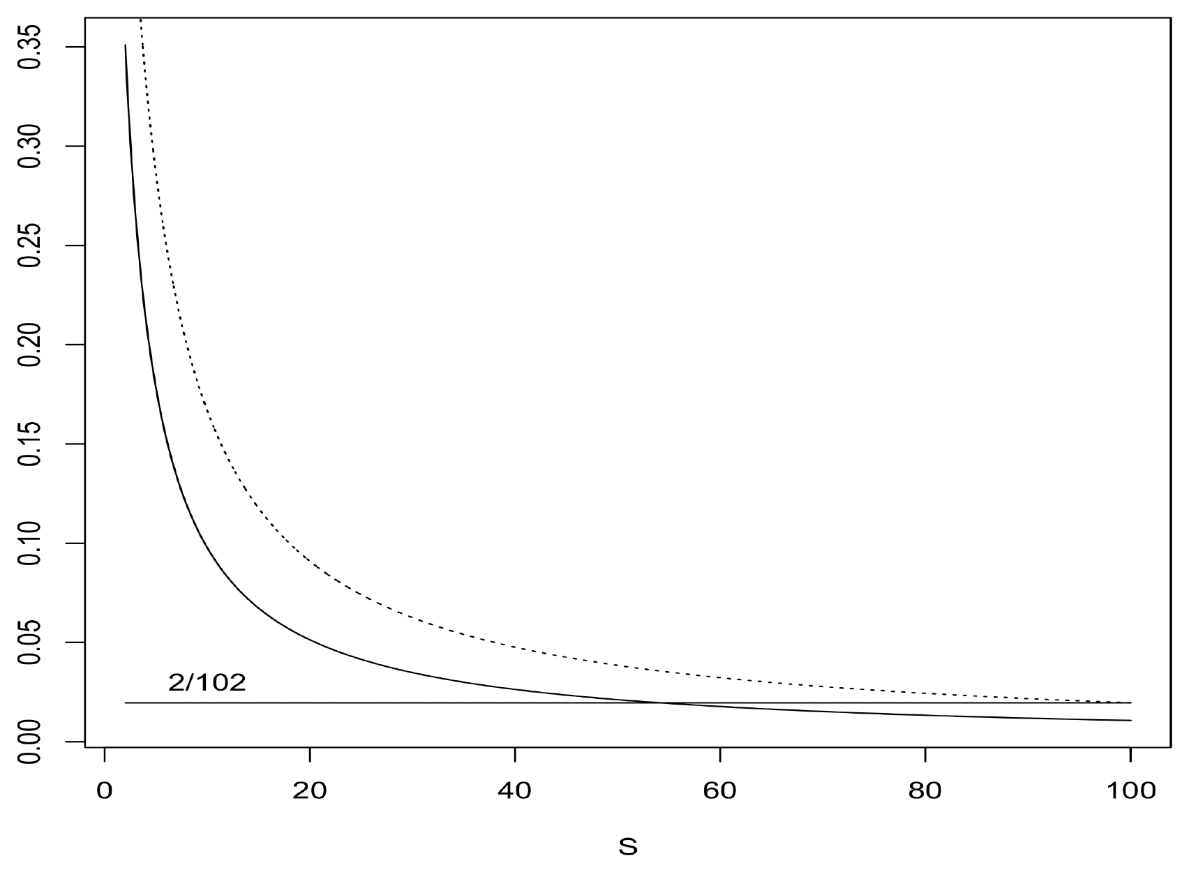
This result reveals the fact that the $L_2$-rate of convergence of $\bar{r}n(\mathbf{X})$ to $r(\mathbf{X})$ depends only on the number $S$ of strong variables, and not on the ambient dimension $d$. The main message of Corollary 1 is that if we are able to properly tune the probability sequences $(p{nj})_{n \geq 1}$ and make them sufficiently fast to track the informative features, then the rate of convergence of the random forests estimate will be of the order $n^{ \frac{-0.75}{S\log 2 + 0.75}}$. This rate is strictly faster than the usual rate $n^{-2/(d+2)}$ as soon as $S\leq \lfloor 0.54d\rfloor$. To understand this point, just recall that the rate $n^{-2/(d+2)}$ is minimax optimal for the class $\mathcal F_d$ (see for example Ibragimov and Khasminskii [30, 31, 32]), seen as a collection of regression functions over $[0,1]^d$, not $[0,1]^S$. However, in our setting, the intrinsic dimension of the regression problem is $S$, not $d$, and the random forests estimate cleverly adapts to the sparsity of the problem. As an illustration, Figure 1 shows the plot of the function $S\mapsto 0.75/(S\log 2+0.75)$ for $S$ ranging from $2$ to $d=100$.

It is noteworthy that the rate of convergence of the $\xi_{nj}$ to 0 (and, consequently, the rate at which the probabilities $p_{nj}$ approach $1/S$ for $j\in \mathcal S$) will eventually depend on the ambient dimension $d$ through the ratio $S/d$. The same is true for the Lipschitz constant $L$ and the factor $\sup_{\mathbf{x} \in [0,1]^d} r^2(\mathbf{x})$ which both appear in Corollary 1. To figure out this remark, remember first that the support of $r$ is contained in $\mathbb{R}^S$, so that the later supremum (respectively, the Lipschitz constant) is in fact a supremum (respectively, a Lipschitz constant) over $\mathbb{R}^S$, not over $\mathbb{R}^d$. Next, denote by $\mathcal C_p(s)$ the collection of functions $\eta:[0,1]^p\to [0,1]$ for which each derivative of order $s$ satisfies a Lipschitz condition. It is well known that the $\varepsilon$-entropy $\log_2(\mathcal N_{\varepsilon})$ of $\mathcal C_p(s)$ is $\Phi(\varepsilon^{-p/(s+1)})$ as $\varepsilon \downarrow 0$ (Kolmogorov and Tihomirov [33]), where $a_n=\Phi(b_n)$ means that $a_n=\mathcal O(b_n)$ and $b_n=\mathcal O(a_n)$. Here we have an interesting interpretation of the dimension reduction phenomenon: Working with Lipschitz functions on $\mathbb{R}^S$ (that is, $s=0$) is roughly equivalent to working with functions on $\mathbb{R}^{d}$ for which all $[(d/S)-1]$-th order derivatives are Lipschitz! For example, if $S=1$ and $d=25$, $(d/S)-1=24$ and, as there are $25^{24}$ such partial derivatives in $\mathbb{R}^{25}$, we note immediately the potential benefit of recovering the "true" dimension $S$.

Remark 2 The reduced-dimensional rate $n^{ \frac{-0.75}{S\log 2 + 0.75}}$ is strictly larger than the $S$-dimensional optimal rate $n^{-2/(S+2)}$, which is also shown in Figure 1 for $S$ ranging from $2$ to $100$. We do not know whether the latter rate can be achieved by the algorithm. $\square$

Remark 3 The optimal parameter $k_n$ of Corollary 1 depends on the unknown distribution of $(\mathbf{X},Y)$, especially on the smoothness of the regression function and the effective dimension $S$. To correct this situation, adaptive (i.e., data-dependent) choices of $k_n$, such as data-splitting or cross-validation, should preserve the rate of convergence of the estimate. Another route we may follow is to analyse the effect of bootstrapping the sample before growing the individual trees (i.e., bagging). It is our belief that this procedure should also preserve the rate of convergence, even for overfitted trees ($k_n \approx n$), in the spirit of [17]. However, such a study is beyond the scope of the present paper. $\square$

Remark 4 For further references, it is interesting to note that Proposition 1 (variance term) is a consequence of aggregation, whereas Proposition 2 (bias term) is a consequence of randomization.

It is also stimulating to keep in mind the following analysis, which has been suggested to us by a referee. Suppose, to simplify, that $Y=r(\mathbf{X})$ (no-noise regression) and that $\sum_{i=1}^n W_{ni}(\mathbf{X},\Theta)=1$ a.s. In this case, the variance term is 0 and we have

$ \bar{r}n(\mathbf{X})=\tilde{r}n(\mathbf{X})=\sum{i=1}^n \mathbb{E}{\Theta}\left[W_{ni}(\Theta, \mathbf{X})\right]Y_i. $

Set $\mathbf Z_n=(Y,Y_1, \cdots,Y_n)$. Then

$ \begin{aligned} &\mathbb{E} \left [\bar{r}_n(\mathbf{X})- r(\mathbf{X})\right]^2 \nonumber\ &\quad =\mathbb{E} \left [ \bar{r}_n(\mathbf{X})- Y\right]^2\nonumber\ & \quad = \mathbb{E} \left [ \mathbb{E} \left [\left ( \bar{r}_n(\mathbf{X})- Y\right)^2 ,|,\mathbf Z_n \right]\right]\nonumber\ &\quad = \mathbb{E} \left [ \mathbb{E} \left [ \left (\bar{r}_n(\mathbf{X})- \mathbb{E} [\bar{r}_n(\mathbf{X}),|,\mathbf Z_n]\right)^2,|,\mathbf Z_n\right]\right]\nonumber\ & \qquad + \mathbb{E}\left [\mathbb{E} [\bar{r}_n(\mathbf{X}),|,\mathbf Z_n]-Y\right]^2. \end{aligned} $

The conditional expectation in the first of the two terms above may be rewritten under the form

$ \mathbb{E} \left[\text{Cov} \left ( \mathbb{E}{\Theta}\left [r_n(\mathbf{X},\Theta)\right],\mathbb{E}{\Theta'}\left [r_n(\mathbf{X},\Theta')\right],|,\mathbf Z_n\right)\right], $

where $\Theta'$ is distributed as, and independent of, $\Theta$. Attention shows that this last term is indeed equal to

$ \mathbb{E} \left[\mathbb{E}_{\Theta,\Theta'} \text{Cov} \left ( r_n(\mathbf{X},\Theta),r_n(\mathbf{X},\Theta') ,|, \mathbf Z_n\right)\right] $

The key observation is that if trees have strong predictive power, then they can be unconditionally strongly correlated while being conditionally weakly correlated. This opens an interesting line of research for the statistical analysis of the bias term, in connection with Amit [34] and Blanchard [35] conditional covariance-analysis ideas. $\square$

3. Discussion

Section Summary: The discussion explains that the theoretical guarantees for the random forests require the splitting procedure to increasingly favor a small set of influential (“strong”) input variables as the sample size grows. It first analyzes an idealized scheme in which these variables are known in advance and shows that drawing an increasing number M_n of candidate coordinates at each node (with M_n growing faster than log n) produces the required selection probabilities. It then describes a practical variant that uses an independent second sample to estimate which coordinates actually reduce variance, thereby approximating the ideal behavior without prior knowledge of the strong variables, while preserving the independence assumptions needed for the proofs.

The results which have been obtained in Section 2 rely on appropriate behavior of the probability sequences $(p_{nj}){n\geq 1}$, $j=1, \cdots,d$. We recall that these sequences should be in $(0,1)$ and obey the constraints $p{nj}=(1/S)(1+\xi_{nj})$ for $j\in \mathcal S$ (and $p_{nj}=\xi_{nj}$ otherwise), where the $(\xi_{nj})_{n\geq 1}$ tend to $0$ as $n$ tends to infinity. In other words, at each step of the construction of the individual trees, the random procedure should track and preferentially cut the strong coordinates. In this more informal section, we briefly discuss a random mechanism for inducing such probability sequences.

Suppose, to start with an imaginary scenario, that we already know which coordinates are strong, and which are not. In this ideal case, the random selection procedure described in the introduction may be easily made more precise as follows. A positive integer $M_n$—possibly depending on $n$—is fixed beforehand and the following splitting scheme is iteratively repeated at each node of the tree:

1. Select at random, with replacement, $M_n$ candidate coordinates to split on. {#11}
2. If the selection is all weak, then choose one at random to split on. If there is more than one strong variable elected, choose one at random and cut. {#22}

Within this framework, it is easy to see that each coordinate in $\mathcal S$ will be cut with the "ideal" probability

$ p_n^{\star}=\frac{1}{S}\left[ 1-\left(1-\frac{S}{d}\right)^{M_n}\right]. $

Though this is an idealized model, it already gives some information about the choice of the parameter $M_n$, which, in accordance with the results of Section 2 (Corollary 1), should satisfy

$ \left(1-\frac{S}{d}\right)^{M_n}\log n \to 0 \quad \text{as } n \to \infty. $

This is true as soon as

$ M_n\to \infty \quad \text{and} \quad \frac{M_n}{\log n} \to \infty \quad \text{as } n \to \infty. $

This result is consistent with the general empirical finding that $M_n$ (called mtry in the R package RandomForests) does not need to be very large (see, for example, Breiman [4]), but not with the widespread belief that $M_n$ should not depend on $n$. Note also that if the $M_n$ features are chosen at random without replacement, then things are even more simple since, in this case, $p^{\star}_n=1/S$ for all $n$ large enough.

In practice, we have only a vague idea about the size and content of the set $\mathcal S$. However, to circumvent this problem, we may use the observations of an independent second set $\mathcal D'_n$ (say, of the same size as $\mathcal D_n)$ in order to mimic the ideal split probability $p_n^{\star}$. To illustrate this mechanism, suppose—to keep things simple—that the model is linear, i.e.,

$ Y=\sum_{j \in \mathcal S} a_j X^{(j)}+\varepsilon, $

where $\mathbf{X}=(X^{(1)}, \cdots, X^{(d)})$ is uniformly distributed over $[0,1]^d$, the $a_j$ are non-zero real numbers, and $\varepsilon$ is a zero-mean random noise, which is assumed to be independent of $\mathbf{X}$ and with finite variance. Note that, in accordance with our sparsity assumption, $r(\mathbf{X})=\sum_{j \in \mathcal S} a_j X^{(j)}$ depends on $\mathbf{X}_{\mathcal S}$ only.

Assume now that we have done some splitting and arrived at a current set of terminal nodes. Consider any of these nodes, say $A=\prod_{j=1}^d A_j$, fix a coordinate $j\in {1, \cdots, d}$, and look at the weighted conditional variance $\mathbb{V}[Y|X^{(j)} \in A_j],\mathbb{P}(X^{(j)}\in A_j)$. It is a simple exercise to prove that if $\mathbf{X}$ is uniform and $j \in \mathcal S$, then the split on the $j$-th side which most decreases the weighted conditional variance is at the midpoint of the node, with a variance decrease equal to $a_j^2/16>0$. On the other hand, if $j\in \mathcal W$, the decrease of the variance is always 0, whatever the location of the split.

On the practical side, the conditional variances are of course unknown, but they may be estimated by replacing the theoretical quantities by their respective sample estimates (as in the CART procedure, see Breiman et al. ([4], Chapter 8) for a thorough discussion) evaluated on the second sample $\mathcal D'_n$. This suggests the following procedure, at each node of the tree:

1. Select at random, with replacement, $M_n$ candidate coordinates to split on. {#one}
2. For each of the $M_n$ elected coordinates, calculate the best split, i.e., the split which most decreases the within-node sum of squares on the second sample $\mathcal D'_n$. {#two}
3. Select one variable at random among the coordinates which output the best within-node sum of squares decreases, and cut. {#three}

This procedure is indeed close to what the random forests algorithm does. The essential difference is that we suppose to have at hand a second sample $\mathcal D'n$, whereas the original algorithm performs the search of the optimal cuts on the original observations $\mathcal D_n$. This point is important, since the use of an extra sample preserves the independence of $\Theta$ (the random mechanism) and $\mathcal D_n$ (the training sample). We do not know whether our results are still true if $\Theta$ depends on $\mathcal D_n$ (as in the CART algorithm), but the analysis does not appear to be simple. Note also that, at step 3, a threshold (or a test procedure, as suggested in Amaratunga et al. [36]) could be used to choose among the most significant variables, whereas the actual algorithm just selects the best one. In fact, depending on the context and the actual cut selection procedure, the informative probabilities $p{nj}$ ($j\in \mathcal S$) may obey the constraints $p_{nj} \to p_j$ as $n \to \infty$ (thus, $p_j$ is not necessarily equal to $1/S$), where the $p_{j}$ are positive and satisfy $\sum_{j\in\mathcal S}p_{j}=1$. This should not affect the results of the article.

This empirical randomization scheme leads to complicate probabilities of cuts which, this time, vary at each node of each tree and are not easily amenable to analysis. Nevertheless, observing that the average number of cases per terminal node is about $n/k_n$, it may be inferred by the law of large numbers that each variable in $\mathcal S$ will be cut with probability

$ p_{nj}\approx \frac{1}{S}\left 1-\left(1-\frac{S}{d}\right)^{M_n}\right, $

where $\zeta_{nj}$ is of the order $\mathcal{O}(k_n/ n)$, a quantity which anyway goes fast to 0 as $n$ tends to infinity. Put differently, for $j \in \mathcal S$,

$ p_{nj}\approx\frac{1}{S}\left(1+\xi_{nj}\right), $

where $\xi_{nj}$ goes to $0$ and satisfies the constraint $\xi_{nj}\log n \to 0$ as $n$ tends to infinity, provided $k_n\log n /n \to 0$, $M_n \to \infty$ and $M_n/\log n \to \infty$. This is coherent with the requirements of Corollary 1. We realize however that this is a rough approach, and that more theoretical work is needed here to fully understand the mechanisms involved in CART and Breiman's original randomization process.

It is also noteworthy that random forests use the so-called out-of-bag samples (i.e., the bootstrapped data which are not used to fit the trees) to construct a variable importance criterion, which measures the prediction strength of each feature (see, e.g., Genuer et al. [11]). As far as we are aware, there is to date no systematic mathematical study of this criterion. It is our belief that such a study would greatly benefit from the sparsity point of view developed in the present paper, but is unfortunately much beyond its scope. Lastly, it would also be interesting to work out and extend our results to the context of unsupervised learning of trees. A good route to follow with this respect is given by the strategies outlined in Amit and Geman ([5], Section 5.5).

4. A small simulation study

Section Summary: The section presents a modest simulation study on synthetic data to illustrate how random forests behave in high-dimensional settings. Three regression models were examined, each with only a few truly relevant variables amid many irrelevant ones; experiments tracked how often each variable was chosen for splits and measured prediction error as sample size and dimension varied. Results showed that, with more data, splits concentrate on the informative variables, error rates become largely independent of the ambient dimension, and a simplified fixed-node version of the algorithm performs similarly to standard random forests.

Even though the first vocation of the present paper is theoretical, we offer in this short section some experimental results on synthetic data. Our aim is not to provide a thorough practical study of the random forests method, but rather to illustrate the main ideas of the article. As for now, we let $\mathcal{U}([0,1]^d)$ (respectively, $\mathcal N(0,1)$) be the uniform distribution over $[0,1]^d$ (respectively, the standard Gaussian distribution). Specifically, three models were tested:

1. [Sinus] For $\mathbf{x} \in [0,1]^d$, the regression function takes the form

$ r(\mathbf{x})= 10 \sin(10 \pi x^{(1)}). $

We let $Y = r(\mathbf{X}) + \varepsilon$ and $\mathbf{X}\sim\mathcal{U}([0,1]^d)$ ($d\geq 1$), with $\varepsilon\sim\mathcal{N}(0,1)$. 2. [Friedman #1] This is a model proposed in Friedman [37]. Here,

$ r(\mathbf{x})=10 \sin(\pi x^{(1)} x^{(2)}) + 20(x^{(3)}-.05)^2 + 10 x^{(4)} + 5 x^{(5)} $

and $Y = r(\mathbf{X}) + \varepsilon$, where $\mathbf{X}\sim\mathcal{U}([0,1]^d)$ ($d\geq 5$) and $\varepsilon\sim\mathcal{N}(0,1)$. 3. [Tree] In this example, we let $Y = r(\mathbf{X}) + \varepsilon$, where $\mathbf{X}\sim\mathcal{U}([0,1]^d)$ ($d\geq 5$), $\varepsilon\sim\mathcal{N}(0,1)$ and the function $r$ has itself a tree structure. This tree-type function, which is shown in Figure 2, involves only five variables.

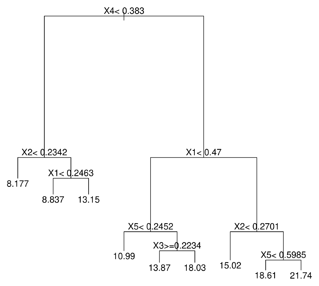
We note that, although the ambient dimension $d$ may be large, the effective dimension of model 1 is $S=1$, whereas model 2 and model 3 have $S=5$. In other words, $\mathcal S={1}$ for model 1, whereas $\mathcal S={1, \cdots, 5}$ for model 2 and model 3. Observe also that, in our context, the model Tree should be considered as a "no-bias" model, on which the random forests algorithm is expected to perform well.

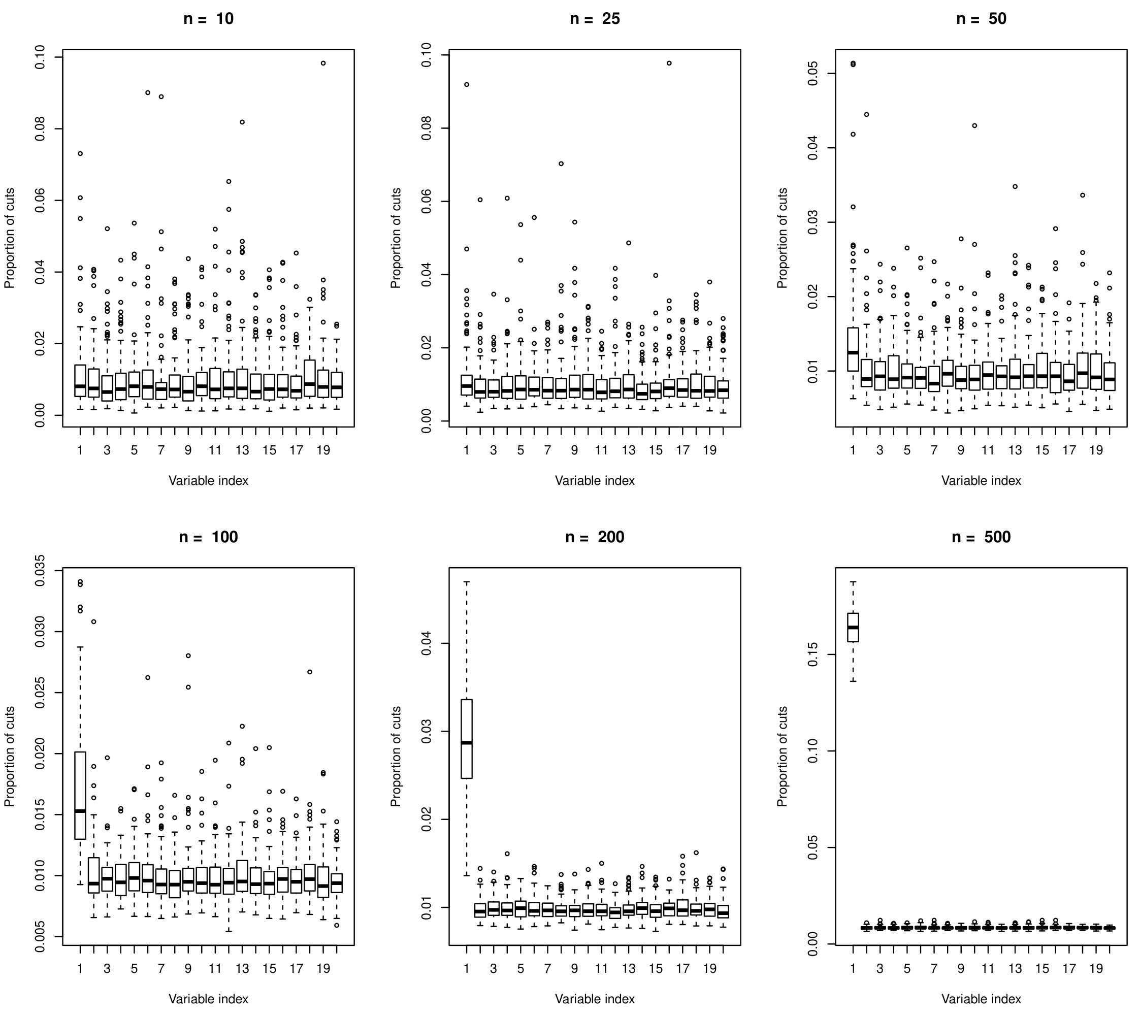
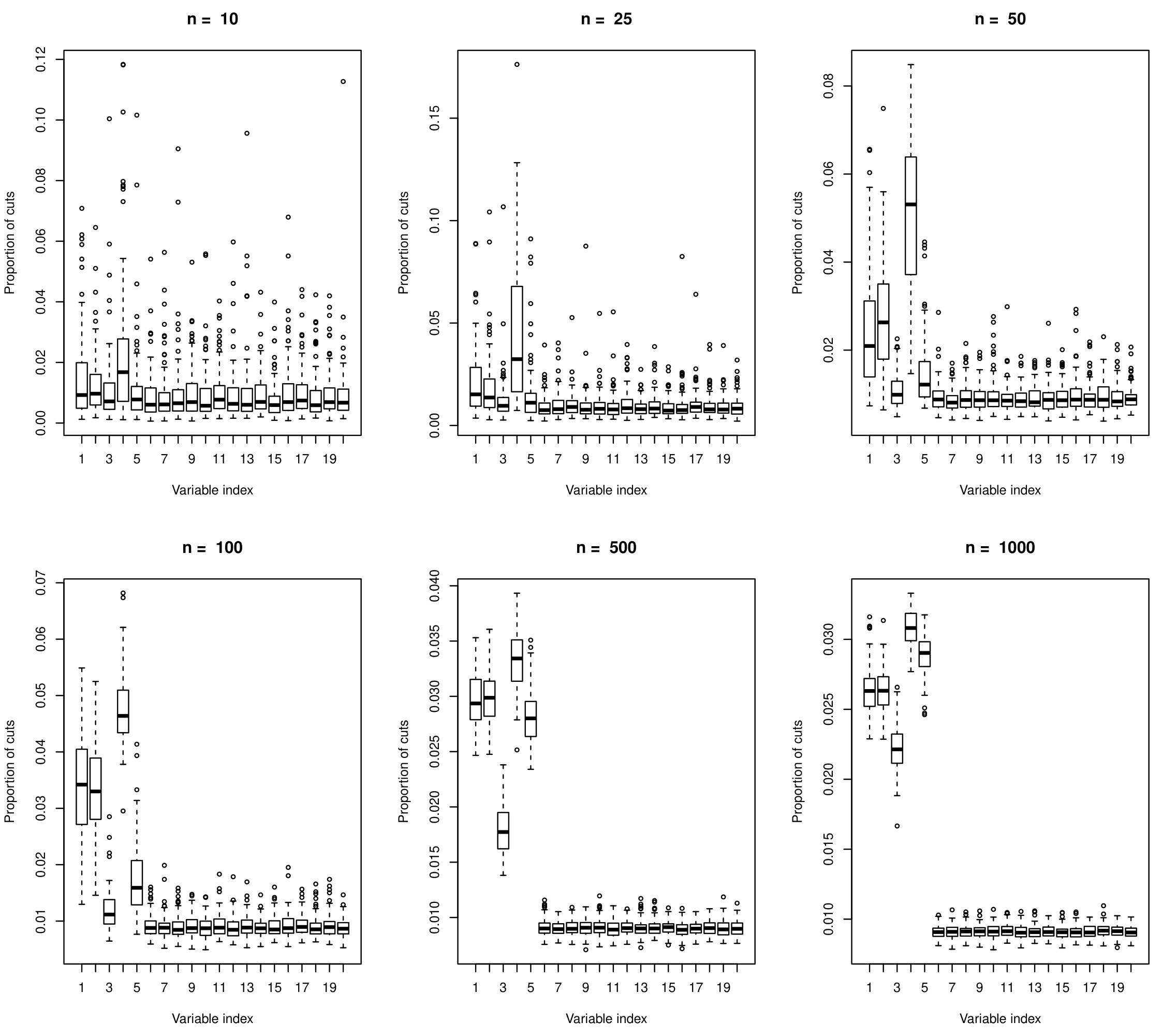
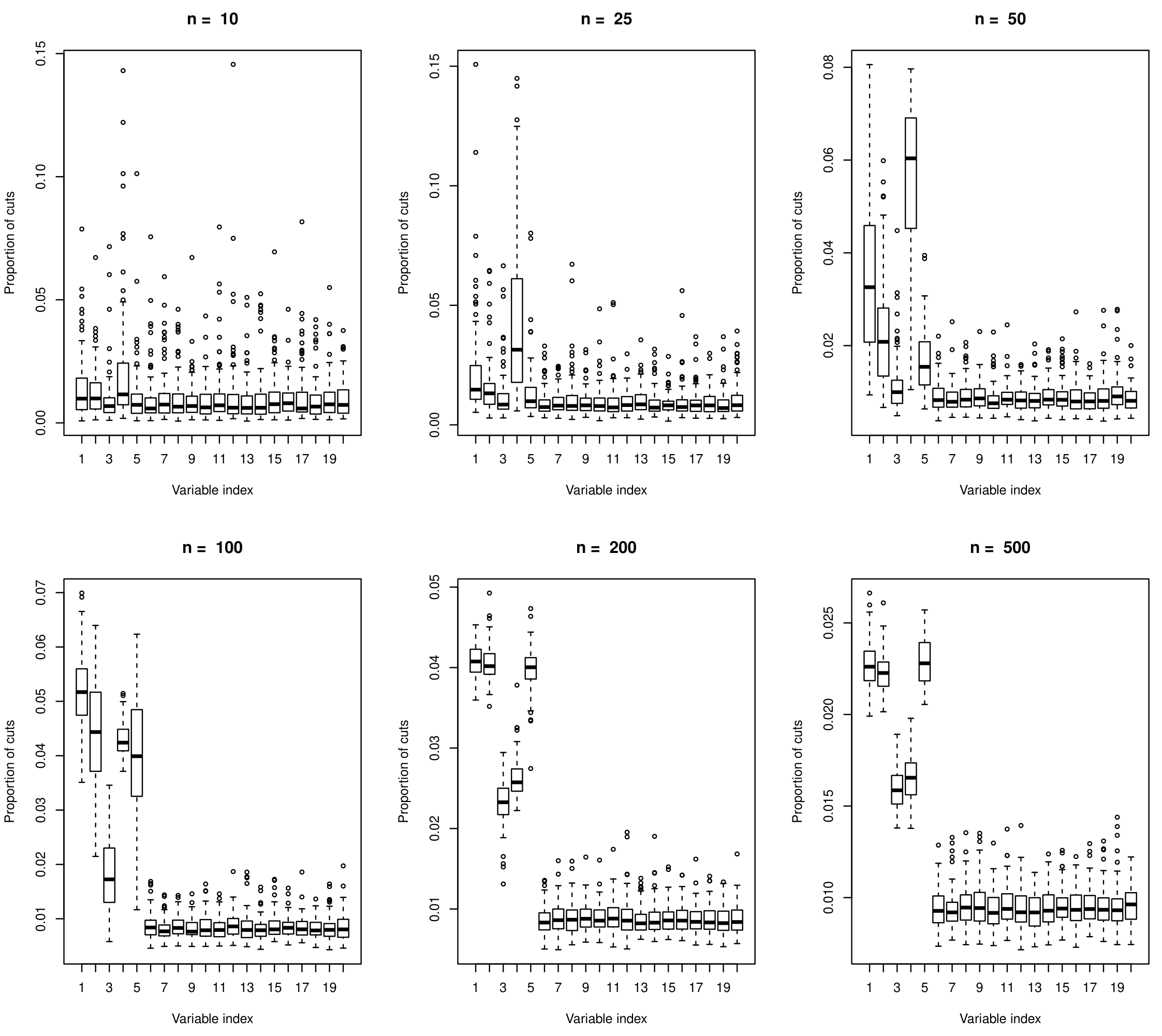
In a first series of experiments, we let $d=100$ and, for each of the three models and different values of the sample size $n$, we generated a learning set of size $n$ and fitted a forest ($10,000$ trees) with $\texttt{mtry} = d$. For $j=1, \cdots, d$, the ratio (number of times the $j$-th coordinate is split)/(total number of splits over the forest) was evaluated, and the whole experiment was repeated 100 times. Figure 3, Figure 4 and Figure 5 report the resulting boxplots for each of the first twenty variables and different values of $n$. These figures clearly enlighten the fact that, as $n$ grows, the probability of cuts does concentrate on the informative variables only and support the assumption that $\xi_{nj}\to0$ as $n\to \infty$ for each $j\in \mathcal S$.

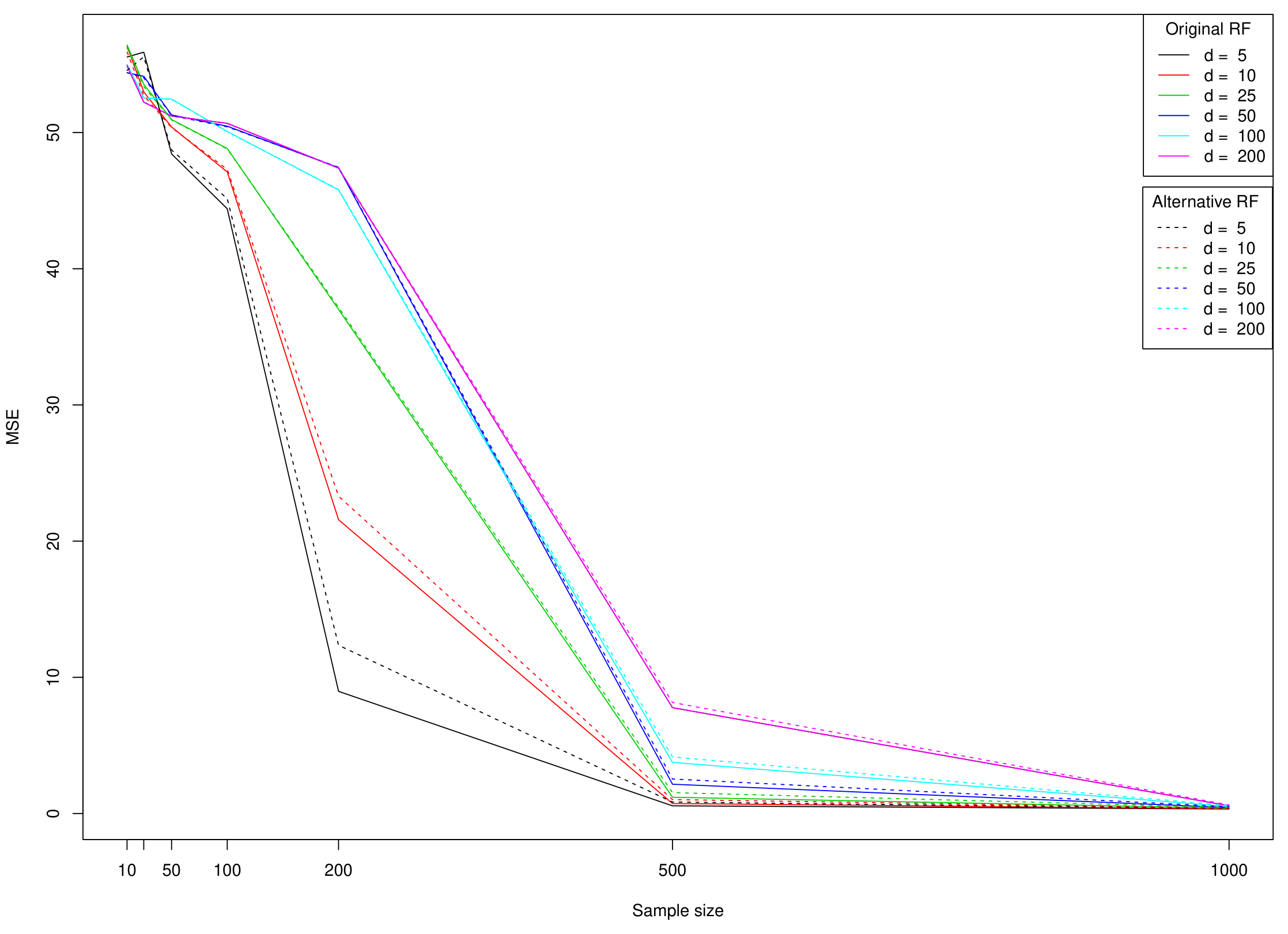
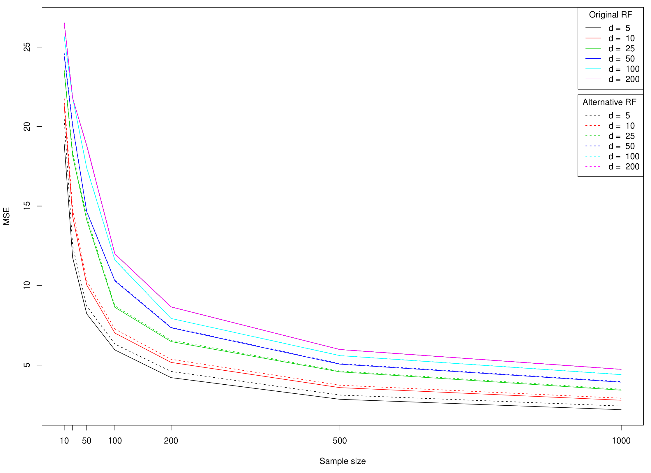
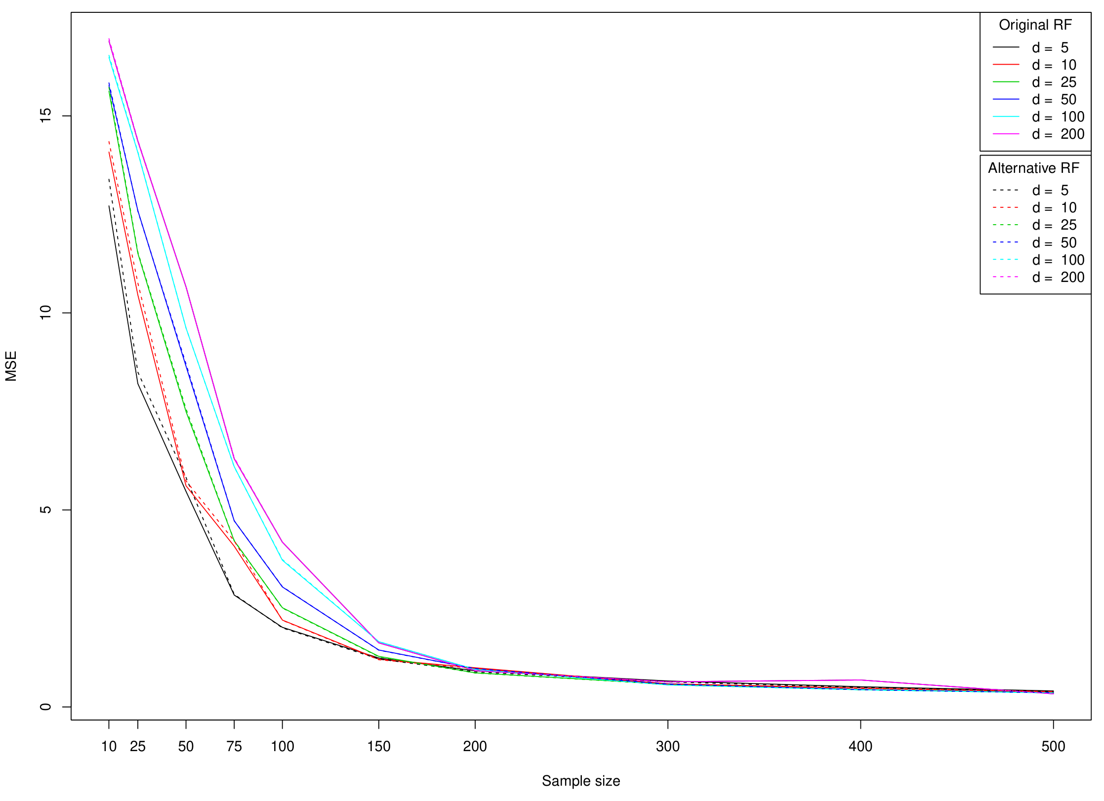
Next, in a second series of experiments, for each model, for different values of $d$ and for sample sizes $n$ ranging from 10 to 1000, we generated a learning set of size $n$, a test set of size $50,000$ and evaluated the mean squared error (MSE) of the random forests (RF) method via the Monte Carlo approximation

$ \text{MSE} \approx \frac {1}{50,000} \sum_{j=1}^{50,000} \left[\text{RF}(\text{test data #j}) - r(\text{test data #j}) \right]^2. $

All results were averaged over 100 data sets. The random forests algorithm was performed with the parameter mtry automatically tuned by the R package RandomForests, $1000$ random trees and the minimum node size set to $5$ (which is the default value for regression). Besides, in order to compare the "true" algorithm with the approximate model discussed in the present document, an alternative method was also tested. This auxiliary algorithm has characteristics which are identical to the original ones (same mtry, same number of random trees), with the notable difference that now the maximum number of nodes is fixed beforehand. For the sake of coherence, since the minimum node size is set to 5 in the RandomForests package, the number of terminal nodes in the custom algorithm was calibrated to $\lceil n/5\rceil$. It must be stressed that the essential difference between the standard random forests algorithm and the alternative one is that the number of cases in the final leaves is fixed in the former, whereas the latter assumes a fixed number of terminal nodes. In particular, in both algorithms, cuts are performed using the actual sample, just as CART does. To keep things simple, no data-splitting procedure has been incorporated in the modified version.

Figure 6, Figure 7 and Figure 8 illustrate the evolution of the MSE value with respect to $n$ and $d$, for each model and the two tested procedures. First, we note that the overall performance of the alternative method is very similar to the one of the original algorithm. This confirms our idea that the model discussed in the present paper is a good approximation of the authentic Breiman's forests. Next, we see that for a sufficiently large $n$, the capabilities of the forests are nearly independent of $d$, in accordance with the idea that the (asymptotic) rate of convergence of the method should only depend on the "true" dimensionality $S$ (Theorem 2). Finally, as expected, it is noteworthy that both algorithms perform well on the third model, which has been precisely designed for a tree-structured predictor.

5. Proofs

Section Summary: This section lays out the mathematical groundwork and detailed arguments needed to establish consistency results for a random forest-style regression estimator. It begins by stating two basic facts about how the algorithm randomly partitions the input space into rectangular cells of shrinking size, along with a remark on how the arguments extend beyond uniform data distributions. The remainder derives the two main claims: first that cell diameters shrink to zero while the number of sample points per cell grows without bound (which together imply consistency), and second that a certain averaged version of the estimator has vanishing variance.

Throughout this section, we will make repeated use of the following two facts.

########## {caption="Fact 1"}

Let $K_{nj}(\mathbf{X},\Theta)$ be the number of times the terminal node $A_n(\mathbf{X},\Theta)$ is split on the $j$-th coordinate ($j=1, \cdots, d$). Then, conditionally on $\mathbf{X}$, $K_{nj}(\mathbf{X},\Theta)$ has binomial distribution with parameters $\lceil{\log_2 k_n}\rceil$ and $p_{nj}$ (by independence of $\mathbf{X}$ and $\Theta$). Moreover, by construction,

$ \sum_{j=1}^d K_{nj}(\mathbf{X},\Theta)= \lceil{\log_2 k_n}\rceil. $

Recall that we denote by $N_n(\mathbf{X},\Theta)$ the number of data points falling in the same cell as $\mathbf{X}$, i.e.,

$ N_n(\mathbf{X},\Theta)= \sum_{i=1}^n \mathbf 1_{[\mathbf{X}_i\in A_n(\mathbf{X},\Theta)]}. $

Let $\lambda$ be the Lebesgue measure on $[0,1]^d$.

########## {caption="Fact 2"}

By construction,

$ \lambda \left (A_n(\mathbf{X},\Theta)\right)=2^{-\lceil{\log_2 k_n}\rceil}. $

In particular, if $\mathbf{X}$ is uniformly distributed on $[0,1]^d$, then the distribution of $N_n(\mathbf{X},\Theta)$ conditionally on $\mathbf{X}$ and $\Theta$ is binomial with parameters $n$ and $2^{-\lceil{\log_2 k_n}\rceil}$ (by independence of the random variables $\mathbf{X}, \mathbf{X}_1, \cdots, \mathbf{X}_n, \Theta$).

Remark 5 If $\mathbf{X}$ is not uniformly distributed but has a probability density $f$ on $[0,1]^d$, then, conditionally on $\mathbf{X}$ and $\Theta$, $N_n(\mathbf{X},\Theta)$ is binomial with parameters $n$ and $\mathbb{P}(\mathbf{X}_1 \in A_n(\mathbf{X},\Theta),|, \mathbf{X},\Theta)$. If $f$ is bounded from above and from below, this probability is of the order $\lambda \left (A_n(\mathbf{X},\Theta)\right)=2^{-\lceil{\log_2 k_n}\rceil}$, and the whole approach can be carried out without difficulty. On the other hand, for more general densities, the binomial probability depends on $\mathbf{X}$, and this makes the analysis significantly harder. $\square$

5.1 Proof of Theorem 1

Observe first that, by Jensen's inequality,

$ \begin{aligned} \mathbb{E} \left [\bar{r}n(\mathbf{X})-r(\mathbf{X})\right]^2& =\mathbb{E} \left [ \mathbb{E}{\Theta} \left [r_n(\mathbf{X},\Theta)-r(\mathbf{X})\right]\right]^2\ & \leq \mathbb{E} \left [ r_n(\mathbf{X},\Theta)-r(\mathbf{X})\right]^2. \end{aligned} $

A slight adaptation of Theorem 4.2 in Györfi et al. [29] shows that $\bar{r}_n$ is consistent if both $\text{diam}(A_n(\mathbf{X},\Theta)) \to 0$ in probability and $N_n(\mathbf{X},\Theta) \to \infty$ in probability.

Let us first prove that $N_n(\mathbf{X},\Theta) \to \infty$ in probability. To see this, consider the random tree partition defined by $\Theta$, which has by construction exactly $2^{\lceil{\log_2 k_n}\rceil}$ rectangular cells, say $A_1,\ldots,A_{2^{\lceil{\log_2 k_n}\rceil}}$. Let $N_1,\ldots,N_{2^{\lceil{\log_2 k_n}\rceil}}$ denote the number of observations among $\mathbf{X}, \mathbf{X}_1,\ldots, \mathbf{X}_n$ falling in these $2^{\lceil{\log_2 k_n}\rceil}$ cells, and let $\mathcal C={\mathbf{X}, \mathbf{X}_1,\ldots, \mathbf{X}n}$ denote the set of positions of these $n+1$ points. Since these points are independent and identically distributed, fixing the set $\mathcal C$ and $\Theta$, the conditional probability that $\mathbf{X}$ falls in the $\ell$-th cell equals $N{\ell}/(n+1)$. Thus, for every fixed $M\geq 0$,

$ \begin{aligned} \mathbb{P} \left(N_n(\mathbf{X},\Theta) < M\right) & = \mathbb{E} \left[\mathbb{P} \left(N_n(\mathbf{X},\Theta) < M,|, \mathcal C,\Theta\right) \right] \ &= \mathbb{E} \left[ \sum_{\ell=1, \cdots, 2^{\lceil{\log_2 k_n}\rceil} : N_{\ell} < M} \frac{N_{\ell}}{n+1} \right]\ & \leq \frac{M2^{\lceil{\log_2 k_n}\rceil}}{n+1}\ & \leq \frac{2Mk_n}{n+1}, \end{aligned} $

which converges to 0 by our assumption on $k_n$.

It remains to show that $\text{diam}(A_n(\mathbf{X},\Theta)) \to 0$ in probability. To this aim, let $V_{nj}(\mathbf{X},\Theta)$ be the size of the $j$-th dimension of the rectangle containing $\mathbf{X}$. Clearly, it suffices to show that $V_{nj} (\mathbf{X},\Theta) \to 0$ in probability for all $j=1, \cdots, d$. To this end, note that

$ V_{nj} (\mathbf{X},\Theta)\stackrel{\mathcal D}{=}2^{-K_{nj}(\mathbf{X},\Theta)}, $

where, conditionally on $\mathbf{X}$, $K_{nj}(\mathbf{X},\Theta)$ has a binomial $\mathcal B(\lceil{\log_2 k_n}\rceil,p_{nj})$ distribution, representing the number of times the box containing $\mathbf{X}$ is split along the $j$-th coordinate (Fact 1). Thus

$ \begin{aligned} \mathbb{E} \left [V_{nj} (\mathbf{X},\Theta) \right]& =\mathbb{E} \left[2^{-K_{nj}(\mathbf{X},\Theta)}\right]\ & =\mathbb{E} \left[\mathbb{E} \left[2^{-K_{nj}(\mathbf{X},\Theta)},|, \mathbf{X}\right]\right]\ & =(1-p_{nj}/2)^{\lceil{\log_2 k_n}\rceil}, \end{aligned} $

which tends to $0$ as $p_{nj}\log k_n \to \infty$.

5.2 Proof of Proposition 1

Recall that

$ \bar{r}n(\mathbf{X})=\sum{i=1}^n \mathbb{E}{\Theta}\left [W{ni}(\mathbf{X},\Theta)\right] Y_i, $

where

$ W_{ni}(\mathbf{X},\Theta)=\frac{\mathbf 1_{[\mathbf{X}i \in A_n(\mathbf{X},\Theta)]}}{N_n(\mathbf{X},\Theta)},\mathbf 1{\mathcal E_n(\mathbf{X},\Theta)} $

and

$ \mathcal E_n=\left [N_n(\mathbf{X},\Theta) \neq 0 \right ]. $

Similarly,

$ \tilde{r}n(\mathbf{X})= \sum{i=1}^n\mathbb{E}{\Theta}\left [W{ni}(\mathbf{X},\Theta)\right] r({\mathbf{X}}_i). $

We have

$ \begin{aligned} \mathbb{E} \left [\bar{r}n(\mathbf{X})-\tilde{r}n(\mathbf{X}) \right]^2 & = \mathbb{E} \left [\sum{i=1}^n \mathbb{E}{\Theta}\left [W_{ni}(\mathbf{X},\Theta)\right]\left(Y_i-r(\mathbf{X}i)\right)\right]^2\ & = \mathbb{E} \left [\sum{i=1}^n \mathbb{E}{\Theta}^2\left [W{ni}(\mathbf{X},\Theta)\right]\left(Y_i-r(\mathbf{X}i)\right)^2\right]\ & \quad (\text{the cross terms are } 0 \text{ since } \mathbb{E} [Y_i| \mathbf{X}i]=r(\mathbf{X}i))\ & =\mathbb{E} \left [\sum{i=1}^n \mathbb{E}{\Theta}^2\left [W{ni}(\mathbf{X},\Theta)\right]\sigma^2(\mathbf{X}i)\right]\ &\leq \sigma^2 \mathbb{E} \left[ \sum{i=1}^n \mathbb{E}^2_{\Theta} \left[ W_{ni}(\mathbf{X},\Theta) \right] \right]\ &= n \sigma^2 \mathbb{E} \left[\mathbb{E}^2_{\Theta} \left[ W_{n1}(\mathbf{X},\Theta) \right]\right], \end{aligned} $

where we used a symmetry argument in the last equality. Observe now that

$ \begin{aligned} \mathbb{E}^2_{\Theta} \left[ W_{n1}(\mathbf{X},\Theta) \right] &= \mathbb{E}{\Theta} \left[ W{n1}(\mathbf{X},\Theta) \right] \mathbb{E}{\Theta'} \left[ W{n1}(\mathbf{X},\Theta') \right]\ & \qquad (\text{where } \Theta' \text{ is distributed as, and independent of, } \Theta)\ & \quad =\mathbb{E}{\Theta,\Theta'} \left [ W{n1}(\mathbf{X},\Theta)W_{n1}(\mathbf{X},\Theta')\right]\ & \quad =\mathbb{E}{\Theta,\Theta'} \left[\frac{ \mathbf 1{[\mathbf{X}1 \in A_n(\mathbf{X},\Theta)]} \mathbf 1{[\mathbf{X}1 \in A_n(\mathbf{X},\Theta')]}}{N_n(\mathbf{X},\Theta)N_n(\mathbf{X},\Theta')},\mathbf 1{\mathcal E_n(\mathbf{X},\Theta)}\mathbf 1_{\mathcal E_n(\mathbf{X},\Theta')}\right]\ & \quad = \mathbb{E}{\Theta,\Theta'} \left[\frac{ \mathbf 1{[\mathbf{X}1 \in A_n(\mathbf{X},\Theta)\cap A_n(\mathbf{X},\Theta')]}}{N_n(\mathbf{X},\Theta)N_n(\mathbf{X},\Theta')},\mathbf 1{\mathcal E_n(\mathbf{X},\Theta)}\mathbf 1_{\mathcal E_n(\mathbf{X},\Theta')}\right]. \end{aligned} $

Consequently,

$ \mathbb{E} \left [\bar{r}n(\mathbf{X})-\tilde{r}n(\mathbf{X}) \right]^2 \leq n \sigma^2\mathbb{E} \left[\frac{ \mathbf 1{[\mathbf{X}1 \in A_n(\mathbf{X},\Theta)\cap A_n(\mathbf{X},\Theta')]}}{N_n(\mathbf{X},\Theta)N_n(\mathbf{X},\Theta')},\mathbf 1{\mathcal E_n(\mathbf{X},\Theta)}\mathbf 1{\mathcal E_n(\mathbf{X},\Theta')}\right]. $

Therefore

$ \begin{aligned} & \mathbb{E} \left [\bar{r}n(\mathbf{X})-\tilde{r}n(\mathbf{X}) \right]^2 \ & \quad \leq n \sigma^2 \mathbb{E} \left[\frac{ \mathbf 1{[\mathbf{X}1 \in A_n(\mathbf{X},\Theta)\cap A_n(\mathbf{X},\Theta')]}}{\left(1+\sum{i =2}^n \mathbf 1{[\mathbf{X}i \in A_n(\mathbf{X},\Theta)]}\right)\left(1+\sum{i=2}^n \mathbf 1_{[\mathbf{X}i \in A_n(\mathbf{X},\Theta')]}\right)}\right]\ & \quad = n \sigma^2 \mathbb{E} \Bigg[\mathbb{E} \Bigg [\frac{ \mathbf 1{[\mathbf{X}1 \in A_n(\mathbf{X},\Theta)\cap A_n(\mathbf{X},\Theta')]}}{\left(1+\sum{i =2}^n \mathbf 1_{[\mathbf{X}i \in A_n(\mathbf{X},\Theta)]}\right)}\ & \quad \qquad \qquad \qquad \times \frac{1}{\left(1+\sum{i =2}^n \mathbf 1_{[\mathbf{X}i \in A_n(\mathbf{X},\Theta')]}\right)},|, \mathbf{X}, \mathbf{X}1,\Theta,\Theta' \Bigg]\Bigg]\ & \quad = n \sigma^2 \mathbb{E} \Bigg[ \mathbf 1{[\mathbf{X}1 \in A_n(\mathbf{X},\Theta)\cap A_n(\mathbf{X},\Theta')]}\mathbb{E} \Bigg[\frac{ 1}{\left(1+\sum{i =2}^n \mathbf 1{[\mathbf{X}i \in A_n(\mathbf{X},\Theta)]}\right)}\ & \quad \qquad \qquad \qquad \times \frac{1}{\left(1+\sum{i =2}^n \mathbf 1_{[\mathbf{X}i \in A_n(\mathbf{X},\Theta')]}\right)},|, \mathbf{X}, \mathbf{X}1,\Theta,\Theta' \Bigg]\Bigg]\ & \quad = n \sigma^2 \mathbb{E} \Bigg[ \mathbf 1{[\mathbf{X}1 \in A_n(\mathbf{X},\Theta)\cap A_n(\mathbf{X},\Theta')]}\mathbb{E} \Bigg[\frac{ 1}{\left(1+\sum{i =2}^n \mathbf 1{[\mathbf{X}i \in A_n(\mathbf{X},\Theta)]}\right)}\ & \quad \qquad \qquad \qquad \times \frac{1}{\left(1+\sum{i =2}^n \mathbf 1_{[\mathbf{X}_i \in A_n(\mathbf{X},\Theta')]}\right)},|, \mathbf{X},\Theta,\Theta' \Bigg]\Bigg] \end{aligned} $

by the independence of the random variables $\mathbf{X}, \mathbf{X}_1, \cdots, \mathbf{X}_n, \Theta, \Theta'$. Using the Cauchy-Schwarz inequality, the above conditional expectation can be upper bounded by

$ \begin{aligned} & {\mathbb{E}^{1/2} \left [ \frac{1}{\left(1+\sum_{i =2}^n \mathbf 1_{[\mathbf{X}i \in A_n(\mathbf{X},\Theta)]}\right)^2},|, \mathbf{X},\Theta\right ]} \ & \qquad \times {\mathbb{E}^{1/2} \left [ \frac{1}{\left(1+\sum{i =2}^n \mathbf 1_{[\mathbf{X}_i \in A_n(\mathbf{X},\Theta')]}\right)^2},|, \mathbf{X},\Theta'\right ]}\ & \leq \frac{3\times2^{2 \lceil{\log_2 k_n}\rceil}}{n^2}\ & \quad (\text{by Fact FAIT2 and technical Lemma bosq})\ & \leq \frac{12k_n^2}{n^2}. \end{aligned} $

It follows that

$ \begin{aligned} \mathbb{E} \left [\bar{r}_n(\mathbf{X})-\tilde{r}n(\mathbf{X}) \right]^2 &\leq \frac{12\sigma^2k_n^2}{n},\mathbb{E} \left[ \mathbf 1{[\mathbf{X}1 \in A_n(\mathbf{X},\Theta)\cap A_n(\mathbf{X},\Theta')]}\right]\nonumber\ & =\frac{12\sigma^2k_n^2}{n},\mathbb{E} \left [\mathbb{E}{\mathbf{X}1} \left[ \mathbf 1{[\mathbf{X}1 \in A_n(\mathbf{X},\Theta)\cap A_n(\mathbf{X},\Theta')]}\right]\right]\nonumber\ & =\frac{12\sigma^2k_n^2}{n},\mathbb{E} \left [\mathbb{P}{\mathbf{X}_1} \left(\mathbf{X}_1 \in A_n(\mathbf{X},\Theta)\cap A_n(\mathbf{X},\Theta')\right)\right]. \end{aligned} $

Next, using the fact that $\mathbf{X}_1$ is uniformly distributed over $[0,1]^d$, we may write

$ \begin{aligned} \mathbb{P}{\mathbf{X}1} \left(\mathbf{X}1 \in A_n(\mathbf{X},\Theta)\cap A_n(\mathbf{X},\Theta')\right) &= \lambda \left(A_n(\mathbf{X},\Theta)\cap A_n(\mathbf{X},\Theta')\right)\ &= \prod{j=1}^d \lambda \left(A{nj}(\mathbf{X},\Theta)\cap A{nj}(\mathbf{X},\Theta')\right), \end{aligned} $

where

$ A_n(\mathbf{X},\Theta)=\prod_{j=1}^d A_{nj}(\mathbf{X},\Theta)\quad \text{and}\quad A_n(\mathbf{X},\Theta')=\prod_{j=1}^d A_{nj}(\mathbf{X},\Theta'). $

On the other hand, we know (Fact 1) that, for all $j=1, \cdots, d$,

$ \lambda \left(A_{nj}(\mathbf{X},\Theta)\right)\stackrel{\mathcal D}{=}2^{-K_{nj}(\mathbf{X},\Theta)}, $

where, conditionally on $\mathbf{X}$, $K_{nj}(\mathbf{X},\Theta)$ has a binomial $\mathcal B(\lceil{\log_2 k_n}\rceil,p_{nj})$ distribution and, similarly,

$ \lambda \left(A_{nj}(\mathbf{X},\Theta')\right)\stackrel{\mathcal D}{=}2^{-K'_{nj}(\mathbf{X},\Theta')}, $

where, conditionally on $\mathbf{X}$, $K'{nj}(\mathbf{X},\Theta')$ is binomial $\mathcal B(\lceil{\log_2 k_n}\rceil,p{nj})$ and independent of $K_{nj}(\mathbf{X},\Theta)$. In the rest of the proof, to lighten notation, we write $K_{nj}$ and $K'{nj}$ instead of $K{nj}(\mathbf{X},\Theta)$ and $K'_{nj}(\mathbf{X},\Theta')$, respectively. Clearly,

$ \begin{aligned} \lambda \left(A_{nj}(\mathbf{X},\Theta)\cap A_{nj}(\mathbf{X},\Theta')\right) & {\leq} 2^{-\max(K_{nj},K'{nj})}\ & =2^{-K'{nj}}2^{-(K_{nj}-K'{nj})+} \end{aligned} $

and, consequently,

$ \prod_{j=1}^d \lambda \left(A_{nj}(\mathbf{X},\Theta)\cap A_{nj}(\mathbf{X},\Theta')\right) {\leq}2^{-\lceil{\log_2 k_n}\rceil} \prod_{j=1}^d 2^{-(K_{nj}-K'{nj})+} $

(since, by Fact 1, $\sum_{j=1}^d K_{nj}= \lceil{\log_2 k_n}\rceil$). Plugging this inequality into Equation (8) and applying Hölder's inequality, we obtain

$ \begin{aligned} \mathbb{E} \left [\bar{r}n(\mathbf{X})-\tilde{r}n(\mathbf{X}) \right]^2 &\leq \frac{12\sigma^2k_n}{n} \mathbb{E}\left [ \prod{j=1}^d 2^{-(K{nj}-K'{nj})+}\right]\ & = \frac{12\sigma^2k_n}{n} \mathbb{E}\left[\mathbb{E}\left [ \prod_{j=1}^d 2^{-(K_{nj}-K'{nj})+},|, \mathbf{X}\right]\right]\ & \leq \frac{12\sigma^2k_n}{n} \mathbb{E} \left[\prod_{j=1}^d \mathbb{E}^{1/d} \left [2^{-d(K_{nj}-K'{nj})+},|, \mathbf{X}\right]\right]. \end{aligned} $

Each term in the product may be bounded by technical Proposition 1, and this leads to

$ \begin{aligned} \mathbb{E} \left [\bar{r}n(\mathbf{X})-\tilde{r}n(\mathbf{X}) \right]^2 & \leq \frac{288\sigma^2k_n}{\pi n} \prod{j=1}^d \min \left (1, \left [\frac{\pi}{16 \lceil{\log_2 k_n}\rceil p{nj}(1-p_{nj})}\right]^{1/2d}\right)\ & \leq \frac{288\sigma^2k_n}{\pi n} \prod_{j=1}^d \min \left (1, \left [\frac{\pi\log 2}{16(\log k_n)p_{nj}(1-p_{nj})}\right]^{1/2d}\right). \end{aligned} $

Using the assumption on the form of the $p_{nj}$, we finally conclude that

$ \mathbb{E} \left [\bar{r}_n(\mathbf{X})-\tilde{r}_n(\mathbf{X}) \right]^2 \leq C\sigma^2\left(\frac{S^2}{S-1}\right)^{S/2d}\left(1+\xi_n\right)\frac{k_n}{n(\log k_n)^{S/2d}}, $

where

$ C=\frac{288}{\pi}\left(\frac{\pi \log 2}{16}\right)^{S/2d} $

and

$ 1+\xi_n=\prod_{j \in \mathcal S} \left [\left( 1+ \xi_{nj} \right)^{-1} \left (1- \frac{\xi_{nj}}{S-1} \right)^{-1}\right]^{1/2d}. $

Clearly, the sequence $(\xi_n)$, which depends on the ${(\xi_{nj}) : j\in \mathcal S}$ only, tends to $0$ as $n$ tends to infinity.

5.3 Proof of Proposition 2

We start with the decomposition

$ \begin{aligned} &\mathbb{E} \left [ \tilde{r}n(\mathbf{X})- r(\mathbf{X})\right]^2 \ & \quad = \mathbb{E} \Bigg [ \sum{i=1}^n \mathbb{E}{\Theta} \left [W{ni}(\mathbf{X},\Theta)\right] \left( r(\mathbf{X}i)-r(\mathbf{X})\right)\ & \quad \qquad \qquad +\left(\sum{i=1}^n \mathbb{E}{\Theta} \left [W{ni}(\mathbf{X},\Theta)\right]-1\right) r(\mathbf{X})\Bigg]^2\ & \quad \mbox = \mathbb{E}\left[ \mathbb{E}{\Theta} \left [ \sum{i=1}^n W_{ni}(\mathbf{X},\Theta)\left( r(\mathbf{X}i)-r(\mathbf{X})\right)+\left(\sum{i=1}^nW_{ni}(\mathbf{X},\Theta)-1\right) r(\mathbf{X})\right]\right]^2\ & \quad \leq \mathbb{E}\left[ \sum_{i=1}^n W_{ni}(\mathbf{X},\Theta)\left( r(\mathbf{X}i)- r(\mathbf{X})\right)+\left(\sum{i=1}^nW_{ni}(\mathbf{X},\Theta)-1\right) r(\mathbf{X})\right]^2, \end{aligned} $

where, in the last step, we used Jensen's inequality. Consequently,

$ \begin{aligned} &\mathbb{E} \left [ \tilde{r}n(\mathbf{X})-r(\mathbf{X})\right]^2 \nonumber\ & \quad \leq \mathbb{E}\left[ \sum{i=1}^n W_{ni}(\mathbf{X},\Theta)\left(r(\mathbf{X}i)-r(\mathbf{X})\right)\right]^2+ \mathbb{E} \left[ r(\mathbf{X}),\mathbf 1{\mathcal E_n^c(\mathbf{X},\Theta)} \right]^2\nonumber\ & \quad \leq \mathbb{E}\left[ \sum_{i=1}^n W_{ni}(\mathbf{X},\Theta)\left( r(\mathbf{X}i)- r(\mathbf{X})\right)\right]^2+ \left [\sup{\mathbf x \in [0,1]^d} r^2(\mathbf{x} )\right]\mathbb{P}\left (\mathcal E_n^c(\mathbf{X},\Theta)\right) . \end{aligned} $

Let us examine the first term on the right-hand side of Equation (9). Observe that, by the Cauchy-Schwarz inequality,

$ \begin{aligned} & \mathbb{E} \left [ \sum_{i=1}^n W_{ni}(\mathbf{X},\Theta) \left(r(\mathbf{X}i)-r(\mathbf{X})\right)\right]^2\ &\quad \leq \mathbb{E} \left [ \sum{i=1}^n \sqrt{W_{ni}(\mathbf{X},\Theta)}\sqrt{W_{ni}(\mathbf{X},\Theta)} \left| r(\mathbf{X}i)-r(\mathbf{X})\right|\right]^2\ & \quad \leq \mathbb{E} \left [\left ( \sum{i=1}^n W_{ni}(\mathbf{X},\Theta) \right )\left (\sum_{i=1}^n W_{ni}(\mathbf{X},\Theta) \left (r(\mathbf{X}i)-r(\mathbf{X})\right)^2\right)\right]\ & \quad \leq \mathbb{E} \left [\sum{i=1}^n W_{ni}(\mathbf{X},\Theta)\left(r(\mathbf{X}_i)-r(\mathbf{X})\right)^2\right]\ & \qquad \text{(since the weights are subprobability weights)}. \end{aligned} $

Thus, denoting by $| \mathbf{X}|_{\mathcal S}$ the norm of $\mathbf{X}$ evaluated over the components in $\mathcal S$, we obtain

$ \begin{aligned} &\mathbb{E} \left [ \sum_{i=1}^n W_{ni}(\mathbf{X},\Theta) \left( r(\mathbf{X}i)-r(\mathbf{X})\right)\right]^2 \ & \quad \leq \mathbb{E} \left [\sum{i=1}^n W_{ni}(\mathbf{X},\Theta)\left(r^{\star}(\mathbf{X}{i\mathcal S})-r^{\star}(\mathbf{X}{\mathcal S})\right)^2\right]\ & \quad \leq L^2 \sum_{i=1}^n \mathbb{E} \left [W_{ni}(\mathbf{X},\Theta)| \mathbf{X}i-\mathbf{X}|{\mathcal S}^2\right]\ & \quad = nL^2 \mathbb{E} \left [ W_{n1}(\mathbf{X},\Theta)| \mathbf{X}1-\mathbf{X}|{\mathcal S}^2\right]\ & \qquad \text{(by symmetry)}. \end{aligned} $

But

$ \begin{aligned} & \mathbb{E} \left [ W_{n1}(\mathbf{X},\Theta)| \mathbf{X}1-\mathbf{X}|{\mathcal S}^2\right]\ &\quad =\mathbb{E} \left [ | \mathbf{X}1-\mathbf{X}|{\mathcal S}^2 \frac{ \mathbf 1_{[\mathbf{X}1 \in A_n(\mathbf{X},\Theta)]}}{N_n(\mathbf{X},\Theta)},\mathbf 1{\mathcal E_n(\mathbf{X},\Theta)}\right]\ & \quad =\mathbb{E} \left [ | \mathbf{X}1-\mathbf{X}|{\mathcal S}^2 \frac{ \mathbf 1_{[\mathbf{X}1 \in A_n(\mathbf{X},\Theta)]}}{1+\sum{i=2}^n \mathbf 1_{[\mathbf{X}i \in A_n(\mathbf{X}, \Theta)]}}\right]\ &\quad =\mathbb{E} \left [\mathbb{E} \left [ | \mathbf{X}1-\mathbf{X}|{\mathcal S}^2 \frac{ \mathbf 1{[\mathbf{X}1 \in A_n(\mathbf{X},\Theta)]}}{1+\sum{i=2}^n \mathbf 1_{[\mathbf{X}_i \in A_n(\mathbf{X}, \Theta)]}},|, \mathbf{X}, \mathbf{X}_1, \Theta\right] \right]. \end{aligned} $

Thus,

$ \begin{aligned} & \mathbb{E} \left [ W_{n1}(\mathbf{X},\Theta)| \mathbf{X}1-\mathbf{X}|{\mathcal S}^2\right]\ & \quad =\mathbb{E} \left [ | \mathbf{X}1-\mathbf{X}|{\mathcal S}^2\mathbf 1_{[\mathbf{X}1 \in A_n(\mathbf{X},\Theta)]}\mathbb{E} \left [ \frac{ 1}{1+\sum{i=2}^n \mathbf 1_{[\mathbf{X}i \in A_n(\mathbf{X}, \Theta)]}},|, \mathbf{X}, \mathbf{X}1, \Theta\right] \right]\ & \quad =\mathbb{E} \left [ | \mathbf{X}1-\mathbf{X}|{\mathcal S}^2\mathbf 1{[\mathbf{X}1 \in A_n(\mathbf{X},\Theta)]}\mathbb{E} \left [ \frac{1}{1+\sum{i=2}^n \mathbf 1{[\mathbf{X}_i \in A_n(\mathbf{X}, \Theta)]}},|, \mathbf{X}, \Theta\right] \right]\ & \qquad \text{(by the independence of the random variables } \mathbf{X}, \mathbf{X}_1, \cdots, \mathbf{X}_n, \Theta). \end{aligned} $

By Fact 2 and technical Lemma 1,

$ \mathbb{E} \left [ \frac{1}{1+\sum_{i=2}^n \mathbf 1_{[\mathbf{X}_i \in A_n(\mathbf{X}, \Theta)]}},|, \mathbf{X},\Theta\right] \leq \frac{2^{\lceil{\log_2 k_n}\rceil}}{n}\leq \frac{2k_n}{n}. $

Consequently,

$ \begin{aligned} &\mathbb{E} \left [ \sum_{i=1}^n W_{ni}(\mathbf{X},\Theta) \left(r(\mathbf{X}i)-r(\mathbf{X})\right)\right]^2\ & \quad \leq 2L^2k_n\mathbb{E} \left [ | \mathbf{X}1-\mathbf{X}|{\mathcal S}^2\mathbf 1{[\mathbf{X}_1 \in A_n(\mathbf{X},\Theta)]}\right]. \end{aligned} $

Letting

$ A_n(\mathbf{X},\Theta)=\prod_{j=1}^d A_{nj}(\mathbf{X},\Theta), $

we obtain

$ \begin{aligned} & \mathbb{E} \left [ \sum_{i=1}^n W_{ni}(\mathbf{X},\Theta) \left( r(\mathbf{X}i)- r(\mathbf{X})\right)\right]^2\ & \quad \leq 2L^2k_n\sum{j \in \mathcal S} \mathbb{E} \left [ | \mathbf{X}1^{(j)}-\mathbf{X}^{(j)}|^2\mathbf 1{[\mathbf{X}1 \in A_n(\mathbf{X},\Theta)]}\right]\ & \quad = 2L^2k_n \sum{j \in \mathcal S} \mathbb{E} \left [ \rho_j(\mathbf{X}, \mathbf{X}1,\Theta) \mathbb{E}{\mathbf{X}_1^{(j)}} \left [ | \mathbf{X}1^{(j)}-\mathbf{X}^{(j)}|^2\mathbf 1{[\mathbf{X}1^{(j)} \in A{nj}(\mathbf{X},\Theta)]}\right]\right] \end{aligned} $

where, in the last equality, we set

$ \rho_j(\mathbf{X}, \mathbf{X}1,\Theta)= \prod{t=1, \cdots ,d, t\neq j} \mathbf 1_{[\mathbf{X}1^{(t)} \in A{nt}(\mathbf{X},\Theta)]}. $

Therefore, using the fact that $\mathbf{X}_1$ is uniformly distributed over $[0,1]^d$,

$ \begin{aligned} & \mathbb{E} \left [ \sum_{i=1}^n W_{ni}(\mathbf{X},\Theta) \left(r(\mathbf{X}i)-r(\mathbf{X})\right)\right]^2\ & \quad \leq 2L^2k_n \sum{j \in \mathcal S} \mathbb{E} \left [ \rho_j(\mathbf{X}, \mathbf{X}1,\Theta) \lambda^3 \left (A{nj}(\mathbf{X},\Theta)\right) \right]. \end{aligned} $

Observing that

$ \begin{aligned} &\lambda \left (A_{nj}(\mathbf{X},\Theta)\right) \times \mathbb{E}_{[\mathbf{X}_1^{(t)},:,t=1, \cdots, d, t\neq j]} \left [\rho_j(\mathbf{X}, \mathbf{X}_1,\Theta)\right]\ & \quad = \lambda \left ( A_n(\mathbf{X}, \Theta)\right)\ & \quad =2^{-\lceil{\log_2 k_n}\rceil}\ & \qquad (\text{Fact FAIT2}), \end{aligned} $

we are led to

$ \begin{aligned} &\mathbb{E} \left [ \sum_{i=1}^n W_{ni}(\mathbf{X},\Theta) \left(r(\mathbf{X}i)-r(\mathbf{X})\right)\right]^2 \ & \quad \leq 2 L^2\sum{j \in \mathcal S} \mathbb{E} \left [\lambda^2 \left (A_{nj}(\mathbf{X},\Theta)\right) \right]\ & \quad =2L^2 \sum_{j \in \mathcal S} \mathbb{E}\left [ 2^{-2K_{nj}(\mathbf{X},\Theta)}\right]\ & \quad =2L^2 \sum_{j \in \mathcal S} \mathbb{E} \left[ \mathbb{E}\left [ 2^{-2K_{nj}(\mathbf{X},\Theta)},|, \mathbf{X}\right]\right], \end{aligned} $

where, conditionally on $\mathbf{X}$, $K_{nj}(\mathbf{X},\Theta)$ has a binomial $\mathcal B(\lceil{\log_2 k_n}\rceil,p_{nj})$ distribution (Fact 1). Consequently,

$ \begin{aligned} & \mathbb{E} \left [ \sum_{i=1}^n W_{ni}(\mathbf{X},\Theta) \left(r(\mathbf{X}i)-r(\mathbf{X})\right)\right]^2\ & \quad \leq 2 L^2\sum{j \in \mathcal S}\left (1-0.75p_{nj}\right)^{\lceil{\log_2 k_n}\rceil}\ & \quad \leq 2 L^2\sum_{j \in \mathcal S}\exp \left ( -\frac{0.75}{\log 2} p_{nj} \log k_n\right)\ & \quad = 2L^2 \sum_{j \in \mathcal S} \frac{1}{k_n^{\frac{0.75}{S\log 2} (1+\xi_{nj})}}\ & \quad \leq \frac{2 SL^2}{k_n^{\frac{0.75}{S\log 2} (1+\gamma_{n})}}, \end{aligned} $

with $\gamma_n=\min_{j\in \mathcal S} \xi_{nj}$.

To finish the proof, it remains to bound the second term on the right-hand side of Equation (9), which is easier. Just note that

$ \begin{aligned} \mathbb{P}\left (\mathcal E_n^c(\mathbf{X},\Theta)\right)& = \mathbb{P}\left (\sum_{i=1}^n \mathbf 1_{[\mathbf{X}i\in A_n(\mathbf{X},\Theta)]}=0\right)\ & =\mathbb{E}\left [ \mathbb{P}\left (\sum{i=1}^n \mathbf 1_{[\mathbf{X}_i\in A_n(\mathbf{X},\Theta)]}=0,|, \mathbf{X},\Theta\right)\right]\ & = \left (1-2^{-\lceil{\log_2 k_n}\rceil}\right)^n\ & \quad (\text{by Fact FAIT2})\ & \leq e^{-n/2k_n}. \end{aligned} $

Putting all the pieces together, we finally conclude that

$ \mathbb{E} \left [ \tilde{r}n(\mathbf{X})-r(\mathbf{X})\right]^2 \leq \frac{2SL^2}{k_n^{\frac{0.75}{S\log 2} (1+\gamma{n})}}

• \left[\sup_{\mathbf x \in [0,1]^d}r^2(\mathbf x)\right]e^{-n/2k_n}, $

as desired.

5.4 Some technical results

The following result is an extension of Lemma 4.1 in Györfi et al. [29]. Its proof is given here for the sake of completeness.

########## {caption="Lemma 1"}

Let $Z$ be a binomial $\mathcal B(N,p)$ random variable, with $p \in (0,1]$. Then

• $(i)$

$ \mathbb{E} \left [ \frac{1}{1+Z}\right]\leq \frac{1}{(N+1)p}. $

• $(ii)$

$ \mathbb{E} \left [\frac{1}{Z}\mathbf 1_{[Z\geq 1]} \right]\leq \frac{2}{(N+1)p}. $

• $(iii)$

$ \mathbb{E} \left [ \frac{1}{1+Z^2}\right]\leq \frac{3}{(N+1)(N+2)p^2}. $

Proof of Lemma 1 To prove statement $(i)$, we write

$ \begin{aligned} \mathbb{E} \left [ \frac{1}{1+Z}\right] & = \sum_{j=0}^N \frac{1}{1+j} {{N}\choose{j}}p^j(1-p)^{N-j}\ & = \frac{1}{(N+1)p} \sum_{j=0}^N {{N+1}\choose{j+1}}p^{j+1}(1-p)^{N-j} \ & \leq \frac{1}{(N+1)p} \sum_{j=0}^{N+1} {{N+1}\choose{j}}p^{j}(1-p)^{N+1-j} \ & = \frac{1}{(N+1)p}. \end{aligned} $

The second statement follows from the inequality

$ \mathbb{E} \left [\frac{1}{Z} \mathbf 1_{[Z\geq 1]} \right]\leq \mathbb{E} \left [\frac{2}{1+Z}\right] $

and the third one by observing that

$ \mathbb{E} \left [\frac{1}{1+Z^2}\right]= \sum_{j=0}^N \frac{1}{1+j^2} {{N}\choose{j}}p^j(1-p)^{N-j}. $

Therefore

$ \begin{aligned} \mathbb{E} \left [\frac{1}{1+Z^2}\right]& = \frac{1}{(N+1)p}\sum_{j=0}^N \frac{1+j}{1+j^2} {{N+1}\choose{j+1}}p^{j+1}(1-p)^{N-j}\ & \leq \frac{3}{(N+1)p}\sum_{j=0}^{N} \frac{1}{2+j} {{N+1}\choose{j+1}}p^{j+1}(1-p)^{N-j}\ & \leq \frac{3}{(N+1)p}\sum_{j=0}^{N+1} \frac{1}{1+j} {{N+1}\choose{j}}p^{j}(1-p)^{N+1-j}\ & \leq \frac{3}{(N+1)(N+2)p^2}\ & \quad (\text{by }(i)). \end{aligned} $

$\square$

########## {caption="Lemma 5.2"}

Let $Z_1$ and $Z_2$ be two independent binomial $\mathcal B(N,p)$ random variables. Set, for all $z \in \mathbb{C}^{\star}$, $\varphi(z)=\mathbb{E} [z^{Z_1-Z_2}]$. Then

• $(i)$ For all $z \in \mathbb{C}^{\star}$,

$ \varphi(z)=\left[p(1-p)(z+z^{-1})+1-2p(1-p)\right]^N. $

• $(ii)$ For all $j\in \mathbb{N}$,

$ \mathbb{P}(Z_1-Z_2=j)=\frac{1}{2\pi i} \int_{\Gamma} \frac{\varphi(z)}{z^{j+1}}\emph{d}z, $

where $\Gamma$ is the positively oriented unit circle.

• $(iii)$ For all $d \geq 1$,

$ \mathbb{E} \left [ 2^{-d(Z_1-Z_2)_+} \right]\leq \frac{24}{\pi} \int_0^1 \exp\left(-4Np(1-p)t^2\right)\emph{d}t. $

Proof of the theorem Statement $(i)$ is clear and $(ii)$ is an immediate consequence of Cauchy's integral formula (Rudin [38]). To prove statement $(iii)$, write

$ \begin{aligned} \mathbb{E} \left [ 2^{-d(Z_1-Z_2)+}\right] &=\sum{j=0}^N 2^{-dj},\mathbb{P}\left ((Z_1-Z_2)+=j\right)\ & = \sum{j=0}^N 2^{-dj},\mathbb{P}\left (Z_1-Z_2=j\right)\ & \leq \sum_{j=0}^{\infty} 2^{-dj},\mathbb{P}\left (Z_1-Z_2=j\right)\ & = \frac{1}{2\pi i} \int_{\Gamma} \frac{\varphi (z)}{z} \sum_{j=0}^\infty \left (\frac{2^{-d}}{z}\right)^j\text{d}z\ & \quad (\text{by statement } (ii))\ & = \frac{1}{2\pi} \int_{-\pi}^{\pi}\frac{\varphi(e^{i\theta})}{1-2^{-d} e^{-i\theta}}\text{d}\theta\ & \quad (\text{by setting }z=e^{i\theta}, \theta \in [-\pi,\pi])\ & =\frac{2^{d-1}}{\pi} \int_{-\pi}^{\pi} \left[1+2p(1-p)(\cos \theta-1)\right]^N\frac{e^{i\theta}}{2^de^{i\theta}-1}\text{d}\theta\ & \quad (\text{by statement } (i)).
\end{aligned} $

Noting that

$ \frac{e^{i\theta}}{2^de^{i\theta}-1} = \frac{2^d-e^{i\theta}}{2^{2d}-2^{d+1}\cos \theta +1}, $

we obtain

$ \begin{aligned} & \mathbb{E} \left [ 2^{-d(Z_1-Z_2)+}\right] \ & \quad \leq \frac{2^{d-1}}{\pi}\int{-\pi}^{\pi}\left[1+2p(1-p)(\cos \theta-1)\right]^N \frac{2^d-\cos \theta}{2^{2d}-2^{d+1}\cos \theta +1}\text{d}\theta. \end{aligned} $

The bound

$ \frac{2^d-\cos \theta}{2^{2d}-2^{d+1}\cos \theta+1} \leq \frac{2^d+1}{(2^d-1)^2} $

leads to

$ \begin{aligned} &\mathbb{E} \left [ 2^{-d(Z_1-Z_2)+}\right] \ &\quad \leq \frac{2^{d-1}(2^d+1)}{\pi (2^d-1)^2} \int{-\pi}^{\pi} \left[1+2p(1-p)(\cos \theta-1)\right]^N\text{d}\theta\ & \quad = \frac{2^{d}(2^d+1)}{\pi (2^d-1)^2} \int_{0}^{\pi} \left[1+2p(1-p)(\cos \theta-1)\right]^N\text{d}\theta\ & \quad = \frac{2^{d}(2^d+1)}{\pi (2^d-1)^2} \int_{0}^{\pi} \left[1-4p(1-p)\sin^2(\theta/2)\right]^N\text{d}\theta\ & \qquad(\cos \theta -1=-2 \sin^2(\theta/2))\ &\quad = \frac{2^{d+1}(2^d+1)}{\pi (2^d-1)^2} \int_{0}^{\pi/2} \left[1-4p(1-p)\sin^2\theta\right]^N\text{d}\theta. \end{aligned} $

Using the elementary inequality $(1-z)^N\leq e^{-Nz}$ for $z\in [0,1]$ and the change of variable

$ t=\tan(\theta/2), $

we finally obtain

$ \begin{aligned} &\mathbb{E} \left [ 2^{-d(Z_1-Z_2)_+}\right] \ & \quad \leq \frac{2^{d+2}(2^d+1)}{\pi(2^d-1)^2} \int_0^1 \exp\left(-\frac{16Np(1-p)t^2}{(1+t^2)^2}\right)\frac{1}{1+t^2}\text{d}t\ & \quad \leq C_d\int_0^1 \exp\left(-4Np(1-p)t^2\right)\text{d}t, \end{aligned} $

with

$ C_d=\frac{2^{d+2}(2^d+1)}{\pi(2^d-1)^2}. $

The conclusion follows by observing that $C_d \leq 24/\pi$ for all $d \geq 1$. $\square$

Evaluating the integral in statement $(iii)$ of the theorem leads to the following proposition:

########## {caption="Proposition 1"}

Let $Z_1$ and $Z_2$ be two independent binomial $\mathcal B(N,p)$ random variables, with $p \in (0,1)$. Then, for all $d\geq 1$,

$ \mathbb{E} \left [ 2^{-d(Z_1-Z_2)_+} \right]\leq \frac{24}{\pi} \min \left (1, \sqrt{\frac{\pi}{16Np(1-p)}}\right). $

Acknowledgments.

I greatly thank the Action Editor and two referees for valuable comments and insightful suggestions, which lead to a substantial improvement of the paper. I would also like to thank my colleague Jean-Patrick Baudry for his precious help on the simulation section.

References

Section Summary: This section compiles dozens of academic citations that form the foundation for a discussion of random forest methods and related ensemble techniques. The listed works include seminal papers by Leo Breiman on bagging and random forests, along with studies on decision tree ensembles, variable selection, and theoretical analyses of consistency and convergence. Additional references cover statistical tools such as the Lasso, nonparametric regression theory, and practical applications in areas like gene expression analysis.

[1] L. Breiman. Consistency for a simple model of random forests. Technical Report 670, UC Berkeley, 2004.

[2] L. Breiman. Bagging predictors. Machine Learning, 24:123–140, 1996.

[3] L. Breiman. Some infinity theory for predictor ensembles. Technical Report 577, UC Berkeley, 2000.

[4] L. Breiman. Random forests. Machine Learning, 45:5–32, 2001.

[5] Y. Amit and D. Geman. Shape quantization and recognition with randomized trees. Neural Computation, 9:1545–1588, 1997.

[6] T.K. Ho. The random subspace method for constructing decision forests. IEEE Transactions on Pattern Analysis and Machine Intelligence, 20:832–844, 1998.

[7] T.G. Dietterich. An experimental comparison of three methods for constructing ensembles of decision trees: Bagging, boosting, and randomization. Machine Learning, 40:139–157, 2000.

[8] V. Svetnik, A. Liaw, C. Tong, J. Culberson, R. Sheridan, and B. Feuston. Random forest: A classification and regression tool for compound classification and QSAR modeling. Journal of Chemical Information and Computer Sciences, 43:1947–1958, 2003.

[9] R. Diaz-Uriarte and S.A. de Andrés. Gene selection and classification of microarray data using random forest. BMC Bioinformatics, 7:1471–2105, 2006.

[10] R. Genuer, J.-M. Poggi, and C. Tuleau. Random Forests: Some methodological insights. arXiv:0811.3619, 2008.

[11] R. Genuer, J.-M. Poggi, and C. Tuleau-Malot. Variable selection using random forests. Pattern Recognition Letters, 31:2225–2236, 2010.

[12] Y. Freund and R. Shapire. Experiments with a new boosting algorithm. In L. Saitta, editor, Machine Learning: Proceedings of the 13th International Conference, pages 148–156, San Francisco, 1996. Morgan Kaufmann.

[13] J. Shawe-Taylor and N. Cristianini. Kernel Methods for Pattern Analysis. Cambridge University Press, Cambridge, 2004.

[14] L. Breiman, J.H. Friedman, R.A. Olshen, and C.J. Stone. Classification and Regression Trees. Wadsworth Statistics/Probability Series, Belmont, 1984.

[15] P. Bühlmann and B. Yu. Analyzing bagging. The Annals of Statistics, 30:927–961, 2002.

[16] A. Buja and W. Stuetzle. Observations on bagging. Statistica Sinica, 16:323–352, 2006.

[17] G. Biau, F. Cérou, and A. Guyader. On the rate of convergence of the bagged nearest neighbor estimate. Journal of Machine Learning Research, 11:687–712, 2010.

[18] Y. Lin and Y. Jeon. Random forests and adaptive nearest neighbors. Journal of the American Statistical Association, 101:578–590, 2006.

[19] G. Biau and L. Devroye. On the layered nearest neighbour estimate, the bagged nearest neighbour estimate and the random forest method in regression and classification. Journal of Multivariate Analysis, 101:2499–2518, 2010.

[20] N. Meinshausen. Quantile regression forests. Journal of Machine Learning Research, 7:983–999, 2006.

[21] G. Biau, L. Devroye, and G. Lugosi. Consistency of ran-dom forests and other averaging classifiers. Journal of Machine Learning Research, 9:2015–2033, 2008.

[22] A.M. Bruckstein, D.L. Donoho, and M. Elad. From sparse solutions of systems of equations to sparse modeling of signals and images. SIAM Review, 51:34–81, 2009.

[23] L.J. van't Veer, H. Dai, M.J. van de Vijver, Y.D. He, A.A.M. Hart, M. Mao, H.L. Peterse, K. van der Kooy, M.J. Marton, A.T. Witteveen, G.J. Schreiber, R.M. Kerkhoven, C. Roberts, P.S. Linsley, R. Bernards, and S.H. Friend. Gene expression profiling predicts clinical outcome of breast cancer. Nature, 415:530–536, 2002.

[24] R. Tibshirani. Regression shrinkage and selection via the Lasso. Journal of the Royal Statistical Society, Series B, 58:267–288, 1996.

[25] E.J. Candès and T. Tao. The Dantzig selector: Statistical estimation when $p$ is much larger than $n$. The Annals of Statistics, 35:2313–2351, 2005.

[26] F. Bunea, A. Tsybakov, and M. Wegkamp. Sparsity oracle inequalities for the Lasso. Electronic Journal of Statistics, 1:169–194, 2007.

[27] P. Bickel, Y. Ritov, and A. Tsybakov. Simultaneous analysis of Lasso and Dantzig selector. The Annals of Statistics, 37:1705–1732, 2009.

[28] L. Devroye, L. Györfi, and G. Lugosi. A Probabilistic Theory of Pattern Recognition. Springer-Verlag, New York, 1996.

[29] L. Györfi, M. Kohler, A. Krzyżak, and H. Walk. A Distribution-Free Theory of Nonparametric Regression. Springer-Verlag, New York, 2002.

[30] I.A. Ibragimov and R.Z. Khasminskii. On nonparametric estimation of regression. Doklady Akademii Nauk SSSR, 252:780–784, 1980.

[31] I.A. Ibragimov and R.Z. Khasminskii. Statistical Estimation: Asymptotic Theory. Springer-Verlag, New York, 1981.

[32] I.A. Ibragimov and R.Z. Khasminskii. On the bounds for quality of nonparametric regression function estimation. Theory of Probability and its Applications, 27:81–94, 1982.

[33] A.N. Kolmogorov and V.M. Tihomirov. $\varepsilon$-entropy and $\varepsilon$-capacity of sets in functional spaces. American Mathematical Society Translations, 17:277–364, 1961.

[34] Y. Amit. 2D Object Detection and Recognition: Models, Algorithms, and Networks. The MIT Press, Cambridge, 2002.

[35] G. Blanchard. Different paradigms for choosing sequential reweighting algorithms. Neural Computation, 16:811–836, 2004.

[36] D. Amaratunga, J. Cabrera, and Y.S. Lee. Enriched random forests. Bioinformatics, 24:2010–2014, 2008.

[37] J.H. Friedman. Multivariate adaptive regression splines. The Annals of Statistics, 19:1–67, 1991.

[38] W. Rudin. Real and Complex Analysis, 3rd Edition. McGraw-Hill, New York, 1987.