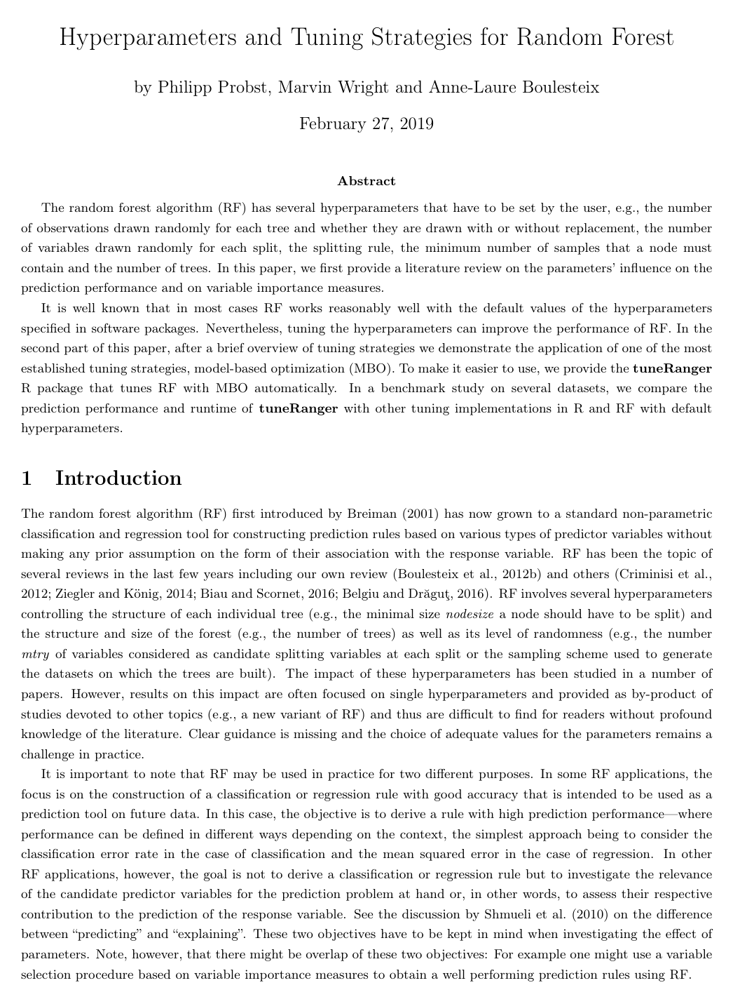
Hyperparameters and tuning strategies for random forest

Philipp ProbstMarvin WrightAnne-Laure Boulesteix

article2018WIREs Data Mining Knowl. Discov.2,141 citations

Evaluates the impact of random forest hyperparameters on prediction performance and variable importance, offering practical tuning strategies and the automated tuneRanger R package to optimize model accuracy.

Listen

Random Forest is widely recognized as an effective and reliable machine learning method that performs reasonably well out of the box. However, practitioners often struggle to determine whether adjusting its core settingsknown as hyperparametersyields enough accuracy gains to justify the extra computational effort. Clear, unified guidance has been lacking in the broader scientific literature regarding how individual parameters behave and how to systematically optimize them.

The article evaluates the practical impact of Random Forest hyperparameters on prediction performance and variable importance measures. It also introduces a practical tuning strategy based on sequential model-based optimization and benchmarks this approach against default configurations and existing automated software packages.

The authors conducted a structured literature review alongside an empirical benchmark across 39 real-world classification datasets from the OpenML platform. The study compared several tuning implementations in R, examining classification error rates, discrimination metrics, probabilistic loss measures, and execution runtimes under repeated cross-validation.

The findings show that Random Forest gains a modest but valuable performance improvement from hyperparameter tuning, reducing classification errors by an average of about 1.3 percentage points compared to default package settings. The number of candidate splitting variables (mtry) is the most influential tuning parameter, whereas the total number of trees is not a tuning parameter and should simply be set sufficiently high (typically 500 to 2,000) until performance stabilizes. Simultaneous tuning of the candidate splitting variables, node size, and sample size consistently outperforms tuning the splitting variables alone. Furthermore, the article demonstrates that using sequential model-based optimization paired with internal out-of-bag validation provides top-tier predictive accuracy while executing significantly faster on larger datasets than cross-validation-based tuning tools like mlrHyperopt.

These results demonstrate that organizations deploying Random Forest in high-stakes environmentssuch as fraud detection, medical risk scoring, or credit underwritingcan capture meaningful predictive and financial gains through systematic tuning. Even moderate reductions in classification error can lower costs and risks substantially. While the default settings serve as a solid baseline, automated optimization avoids the risk of severe underperformance on complex datasets where standard defaults fail to uncover multi-variable interactions.

Practitioners are advised to adopt sequential model-based optimization to simultaneously tune the candidate variable count, node size, and sample size, utilizing the provided tuneRanger tool or comparable out-of-bag optimization workflows. When computational budgets are extremely limited, lightweight options such as tuneRF offer a fast compromise by focusing solely on candidate splitting variables. Future research should prioritize neutral, large-scale empirical studies comparing algorithmic variants and investigating how hyperparameters impact the reliability of variable importance rankings.

The primary limitations include the study's focus on binary classification tasks and the known risk of slight out-of-bag estimation bias in extremely small sample sizes (under 20 observations). Confidence in the findings is high for standard operational dataset sizes, but caution is warranted when interpreting variable importance rankings derived under biased default splitting rules.

Cover for Hyperparameters and tuning strategies for random forest

Abstract

The random forest algorithm (RF) has several hyperparameters that have to be set by the user, e.g., the number of observations drawn randomly for each tree and whether they are drawn with or without replacement, the number of variables drawn randomly for each split, the splitting rule, the minimum number of samples that a node must contain and the number of trees. In this paper, we first provide a literature review on the parameters' influence on the prediction performance and on variable importance measures.

It is well known that in most cases RF works reasonably well with the default values of the hyperparameters specified in software packages. Nevertheless, tuning the hyperparameters can improve the performance of RF. In the second part of this paper, after a brief overview of tuning strategies we demonstrate the application of one of the most established tuning strategies, model-based optimization (MBO). To make it easier to use, we provide the tuneRanger R package that tunes RF with MBO automatically. In a benchmark study on several datasets, we compare the prediction performance and runtime of tuneRanger with other tuning implementations in R and RF with default hyperparameters.

Table of Contents

  • 1 Introduction
  • 2 Literature Review
  • 2.1 Influence on performance
  • 2.1.1 Number of randomly drawn candidate variables (mtry)
  • 2.1.2 Sampling scheme: sample size and replacement
  • 2.1.3 Node size
  • 2.1.4 Number of trees
  • 2.1.5 Splitting rule
  • 2.2 Influence on variable importance
  • 2.2.1 Number of trees
  • 2.2.2 mtry, splitting rule and node size
  • 3 Tuning random forest
  • 3.1 Tunability of random forest
  • 3.2 Evaluation strategies and evaluation measures
  • 3.3 Tuning search strategies
  • 3.4 Existing software implementations
  • 3.5 The tuneRanger package
  • 3.6 Benchmark study
  • 3.6.1 Compared algorithms
  • 3.6.2 Datasets, runtime and evaluation strategy
  • 3.6.3 Results
  • 4 Conclusion and Discussion
  • References

Knowls

  1. Knowl 1 — The tuneRanger Hyperparameter Optimization Algorithm

    algorithm

    The tuneRanger algorithm automates the tuning of random forests implemented in the ranger package by combining sequential model-based optimization (SMBO) with out-of-bag (OOB) evaluation. Given a dataset with nn observations and pp predictor variables, tuneRanger tunes the number of candidate split variables mtrymtry, the minimal node size nodesizenodesize, and the subsample fraction sample.fractionsample.fraction (drawn without replacement).

    Input: Training dataset DD with nn instances and pp features, evaluation metric LL (default: Brier score for classification, MSE for regression), number of trees T=1000T = 1000, initial warm-up iterations ninit=30n_{\text{init}} = 30, SMBO iterations niter=70n_{\text{iter}} = 70
    Output: Recommended hyperparameter configuration θ=(mtry,nodesize,sample.fraction)\theta^* = (mtry^*, nodesize^*, sample.fraction^*) and trained Random Forest model
    Initialize evaluation design set: Deval\mathcal{D}_{\text{eval}} \leftarrow \emptyset
    for i=1i = 1 to ninitn_{\text{init}} do
        Sample mtryiUniform(0,p)mtry_i \sim \text{Uniform}(0, p)
        Sample sample.fractioniUniform(0.2,0.9)sample.fraction_i \sim \text{Uniform}(0.2, 0.9)
        Sample xiUniform(0,1)x_i \sim \text{Uniform}(0, 1) and compute nodesizei(0.2n)xinodesize_i \leftarrow \lfloor (0.2 \cdot n)^{x_i} \rfloor
        Train Random Forest with TT trees on DD using hyperparameters θi=(mtryi,nodesizei,sample.fractioni)\theta_i = (mtry_i, nodesize_i, sample.fraction_i)
        Evaluate loss yi=L(OOB predictions,D)y_i = L(\text{OOB predictions}, D)
        Update design set: DevalDeval{(θi,yi)}\mathcal{D}_{\text{eval}} \leftarrow \mathcal{D}_{\text{eval}} \cup \{(\theta_i, y_i)\}
    end for
    for j=1j = 1 to nitern_{\text{iter}} do
        Fit a surrogate regression model (e.g., Kriging or Random Forest) on Deval\mathcal{D}_{\text{eval}} mapping θy\theta \mapsto y
        Propose candidate configuration θnew\theta_{\text{new}} maximizing an infill criterion (e.g., Expected Improvement)
        Train Random Forest with TT trees on DD using θnew\theta_{\text{new}}
        Evaluate loss ynew=L(OOB predictions,D)y_{\text{new}} = L(\text{OOB predictions}, D)
        Update design set: DevalDeval{(θnew,ynew)}\mathcal{D}_{\text{eval}} \leftarrow \mathcal{D}_{\text{eval}} \cup \{(\theta_{\text{new}}, y_{\text{new}})\}
    end for
    Identify the top 5%5\% evaluations in Deval\mathcal{D}_{\text{eval}} having the lowest loss values
    Compute θ\theta^* as the arithmetic mean of the hyperparameters in the top 5%5\% evaluations, rounding mtrymtry^* and nodesizenodesize^* to the nearest integers
    Train final Random Forest model on DD with θ\theta^*
    return θ\theta^* and final model
  2. Knowl 2 — Benchmark Performance and Ranking of Hyperparameter Tuning Algorithms

    data/table

    Across 39 binary classification datasets from OpenML100, the performance and computational runtime of default random forests (ranger default) were compared against seven tuning methods: four tuneRanger variants optimizing specific evaluation metrics (Mean Misclassification Error MMCE, AUC, Brier score, and Logarithmic Loss), mlrHyperopt (tuning mtry[1,p]mtry \in [1, p] and nodesize[1,10]nodesize \in [1, 10] via 10-fold CV SMBO with 25 iterations), caret (3-point grid search over mtrymtry with 25 bootstrap resamples), and tuneRF (greedy step-wise search over mtrymtry deflating/inflating by factor 2 using OOB error). All forests were evaluated using 2000 trees on 10 CPU cores.

    Algorithm MMCE AUC Brier score Logarithmic Loss Training Runtime (s)
    tuneRangerMMCE 0.0923 0.9191 0.1357 0.2367 903.82
    tuneRangerAUC 0.0925 0.9199 0.1371 0.2450 823.40
    tuneRangerBrier 0.0932 0.9190 0.1325 0.2298 967.21
    tuneRangerLogloss 0.0936 0.9187 0.1330 0.2314 887.83
    mlrHyperopt 0.0934 0.9197 0.1383 0.2364 2713.24
    caret 0.0972 0.9190 0.1439 0.2423 1216.28
    tuneRF 0.0942 0.9174 0.1448 0.2929 862.99
    ranger default 0.1054 0.9128 0.1604 0.2733 3.86

    The corresponding average rank results across the 39 datasets (ranked from 1=best1 = \text{best} to 8=worst8 = \text{worst}) are:

    Algorithm Error rate Rank AUC Rank Brier score Rank Logarithmic Loss Rank Runtime Rank
    tuneRangerMMCE 4.19 4.53 4.41 4.54 5.23
    tuneRangerAUC 3.77 2.56 4.42 4.22 4.63
    tuneRangerBrier 3.13 3.91 1.85 2.69 5.44
    tuneRangerLogloss 3.97 4.04 2.64 2.23 5.00
    mlrHyperopt 4.37 4.68 4.74 4.90 7.59
    caret 5.50 5.24 6.08 5.51 4.36
    tuneRF 4.90 5.08 5.44 6.23 2.76
    ranger default 6.17 5.96 6.42 5.68 1.00

    All tuned versions outperform default ranger on average. Tuning specifically for a targeted metric yields the lowest average error or rank for that metric (e.g., tuneRangerBrier achieves the lowest Brier score of 0.1325 and rank 1.85, and tuneRangerAUC achieves the best AUC rank of 2.56). mlrHyperopt matches tuneRanger accuracy but incurs roughly three times higher training time due to internal 10-fold cross-validation. tuneRF yields high logarithmic loss (0.2929 vs 0.2733 default) due to overly confident probability predictions near 0 and 1.

  3. Knowl 3 — Multidimensional Hyperparameter Tuning Performance Gains over Tuning mtry Alone

    empirical result

    In random forest tuning, simultaneous optimization of multiple structural and sampling hyperparameters yields consistent performance gains compared to optimizing the number of candidate splitting variables mtrymtry in isolation.

    When tuneRanger is configured to tune only mtrymtry versus simultaneously tuning mtrymtry, minimal terminal node size (nodesizenodesize), and the subsample fraction (sample.fractionsample.fraction), joint tuning of all three parameters across 39 benchmark datasets provides the following average improvements:

    • Mean Misclassification Error (MMCE): reduced by 0.0040.004
    • Area Under the ROC Curve (AUC): increased by 0.0020.002
    • Brier score: reduced by 0.0100.010
    • Logarithmic loss: reduced by 0.0140.014
  4. Knowl 4 — Benchmark Experimental Protocol on OpenML-100 Classification Datasets

    experimental setup

    The empirical comparison of random forest hyperparameter tuning algorithms is conducted on 39 binary classification datasets with no missing values selected from the OpenML100 benchmarking suite.

    1. Dataset Categorization: Datasets are classified into "small" (26 datasets) and "big" (13 datasets) using the estimated runtime from the estimateTimeTuneRanger function with 10 CPU cores. If estimated tuning runtime is <10< 10 minutes, the dataset is designated small; otherwise, it is designated big.
    2. Cross-Validation Schemes: Small datasets are evaluated using 10 repeats of 5-fold cross-validation (50 total folds per method). Big datasets are evaluated using a single 5-fold cross-validation.
    3. Base Model Configuration: For all tuning strategies and the default baseline, final random forest models are trained with 2000 trees parallelized across 10 CPU cores via ranger.
    4. Evaluation Measures: Mean Misclassification Error (MMCE), Area Under the ROC Curve (AUC), multiclass Brier score, and logarithmic loss.
    5. Failure and Imputation Handling: If a tuning algorithm fails with error messages on more than 20%20\% of cross-validation iterations for a given dataset (occurring on 2 datasets for mlrHyperopt, 4 for caret, and 3 for tuneRF), the worst result achieved by competing algorithms on that dataset is assigned; otherwise, missing fold results are imputed by the average of the algorithm's successful folds.
  5. Knowl 5 — Random Forest Failure Modes Under Complex Variable Interactions and High Noise Ratios

    empirical result

    Default random forest hyperparameter heuristics (mtry=pmtry = \lfloor \sqrt{p} \rfloor for classification) fail dramatically on datasets exhibiting specific structure, leading to classification error rates approximately 0.150.15 higher than tuned models:

    1. Parity and Complex Feature Interactions (monks-problems-2): In datasets where the outcome depends strictly on higher-order combinations of attributes (e.g., monks-problems-2, with p=6p=6 categorical predictors where outcome y=1y=1 if and only if exactly two predictors equal 2), default mtry=6=2mtry = \lfloor \sqrt{6} \rfloor = 2 fails. Subsets of size 2 rarely contain the required interacting variables simultaneously, causing suboptimal tree partitions. Tuning mtrymtry to the full feature set (mtry=6mtry = 6) allows trees to uncover the exact joint dependency structure, reaching near-perfect accuracy.

    2. High-Dimensional Noise Masking (madelon): In datasets characterized by a small set of true informative features embedded within a large number of noise features (e.g., madelon, containing 20 informative features and 480 non-informative noise features, p=500p=500), default mtry=500=22mtry = \lfloor \sqrt{500} \rfloor = 22 results in individual split candidate sets dominated almost entirely by noise variables. Hyperparameter tuning selects substantially higher mtrymtry values, guaranteeing with high probability that at least one truly predictive variable is evaluated at each node split.

  6. Knowl 6 — Scalability and Speed of Out-of-Bag Evaluation Versus Cross-Validation in Hyperparameter Tuning

    empirical result

    Utilizing out-of-bag (OOB) predictions as the internal loss evaluation during sequential model-based hyperparameter optimization (SMBO) provides a substantial computational speedup over kk-fold cross-validation without loss of generalization performance.

    In SMBO implementations with mlrMBO:

    • mlrHyperopt evaluates each proposed hyperparameter setting via 10-fold cross-validation, requiring 10 separate forest training runs per iteration step across 25 steps (250 model fits total).
    • tuneRanger evaluates each proposed hyperparameter setting using the OOB predictions computed natively during a single forest fit per iteration across 100 steps (30 initial design + 70 SMBO iterations, 100 model fits total).

    Across 39 benchmark datasets, tuneRanger achieves equal or superior predictive performance to mlrHyperopt while reducing average training runtime from 2713.242713.24 seconds (mlrHyperopt) to 823.40823.40--967.21967.21 seconds (tuneRanger). On larger datasets, cross-validation tuning scales approximately 10 times slower than OOB tuning.

  7. Knowl 7 — Variable Selection Bias in Random Forests and Variable Importance Metrics

    theoretical result

    Standard random forest construction and importance metrics exhibit systematic biases dependent on splitting rules, sampling strategies, and predictor variable properties:

    1. Splitting Criterion Bias: Breiman's standard splitting rule (maximizing Gini impurity decrease in classification or variance reduction in regression) favors predictor variables with many possible split points (continuous variables or categorical variables with many categories) over binary or few-level categorical predictors due to multiple hypothesis testing across possible cutpoints.

    2. Variable Importance Distortions:

    • The Gini variable importance measure inherits this split selection bias, assigning elevated importance values to continuous and high-cardinality categorical features even when all predictors are statistically independent of the response.
    • The Permutation variable importance measure is unbiased in expectation for null variables, but exhibits substantially higher variance for variables with many categories.
    1. Unbiased Estimation Strategy: Combining conditional inference forests (which decouple variable selection from split optimization by choosing split variables using global hypothesis test permutation pp-values) with subsampling without replacement (instead of standard bootstrap sampling with replacement) eliminates selection bias and yields reliable variable importance rankings across heterogeneous predictor types.

Coverage note — General literature review summaries of standard Random Forest history and background bagging concepts were omitted as they constitute established prior work rather than novel contributions of this paper.

References

  1. 1.Belgiu, M. and Drăguţ, L. (2016) Random forest in remote sensing: A review of applications and future directions. ISPRS Journal of Photogrammetry and Remote Sensing, 114, 24–31.
  2. 2.Bergstra, J. and Bengio, Y. (2012) Random search for hyper-parameter optimization. Journal of Machine Learning Research, 13, 281–305.
  3. 3.Bernard, S., Heutte, L. and Adam, S. (2009) Influence of hyperparameters on random forest accuracy. In MCS, vol. 5519 of Lecture Notes in Computer Science, 171–180. Springer.
  4. 4.Biau, G. and Scornet, E. (2016) A random forest guided tour. Test, 25, 197–227.
  5. 5.Birattari, M., Yuan, Z., Balaprakash, P. and Stützle, T. (2010) F-Race and iterated F-Race: An overview. In Experimental methods for the analysis of optimization algorithms, 311–336. Springer.
  6. 6.Bischl, B., Casalicchio, G., Feurer, M., Hutter, F., Lang, M., Mantovani, R. G., van Rijn, J. N. and Vanschoren, J. (2017) OpenML benchmarking suites and the OpenML100. ArXiv preprint arXiv:1708.03731. URL: https://arxiv.org/abs/1708.03731.
  7. 7.Bischl, B., Lang, M., Kotthoff, L., Schiffner, J., Richter, J., Studerus, E., Casalicchio, G. and Jones, Z. M. (2016) mlr: Machine learning in R. Journal of Machine Learning Research, 17, 1–5.
  8. 8.Bischl, B., Richter, J., Bossek, J., Horn, D., Thomas, J. and Lang, M. (2017) mlrMBO: A modular framework for model-based optimization of expensive black-box functions. ArXiv preprint arXiv:1703.03373. URL: https://arxiv.org/abs/1703.03373.
  9. 9.Bischl, B., Schiffner, J. and Weihs, C. (2013) Benchmarking local classification methods. Computational Statistics, 28, 2599–2619.
  10. 10.Bohachevsky, I. O., Johnson, M. E. and Stein, M. L. (1986) Generalized simulated annealing for function optimization. Technometrics, 28, 209–217.
  11. 11.Boulesteix, A.-L., Bender, A., Lorenzo Bermejo, J. and Strobl, C. (2012a) Random forest gini importance favours snps with large minor allele frequency: impact, sources and recommendations. Briefings in Bioinformatics, 13, 292–304.
  12. 12.Boulesteix, A.-L., Binder, H., Abrahamowicz, M. and Sauerbrei, W. (2018) On the necessity and design of studies comparing statistical methods. Biometrical Journal, 60, 216–218.
  13. 13.Boulesteix, A.-L., Janitza, S., Kruppa, J. and König, I. R. (2012b) Overview of random forest methodology and practical guidance with emphasis on computational biology and bioinformatics. Wiley Interdisciplinary Reviews: Data Mining and Knowledge Discovery, 2, 493–507.
  14. 14.Boulesteix, A.-L., Wilson, R. and Hapfelmeier, A. (2017) Towards evidence-based computational statistics: lessons from clinical research on the role and design of real-data benchmark studies. BMC Medical Research Methodology, 17, 138.
  15. 15.Breiman, L. (1996) Out-of-bag estimation. Tech. rep., UC Berkeley, Department of Statistics.
  16. 16.— (2001) Random forests. Machine Learning, 45, 5–32.
  17. 17.Casalicchio, G., Bossek, J., Lang, M., Kirchhoff, D., Kerschke, P., Hofner, B., Seibold, H., Vanschoren, J. and Bischl, B. (2017) OpenML: An R package to connect to the machine learning platform OpenML. Computational Statistics, 32, 1–15.
  18. 18.Criminisi, A., Shotton, J., Konukoglu, E. et al. (2012) Decision forests: A unified framework for classification, regression, density estimation, manifold learning and semi-supervised learning. Foundations and Trends® in Computer Graphics and Vision, 7, 81–227.
  19. 19.Díaz-Uriarte, R. and De Andres, S. A. (2006) Gene selection and classification of microarray data using random forest. BMC Bioinformatics, 7, 3.
  20. 20.Fernández-Delgado, M., Cernadas, E., Barro, S. and Amorim, D. (2014) Do we need hundreds of classifiers to solve real world classification problems? Journal of Machine Learning Research, 15, 3133–3181.
  21. 21.Ferri, C., Hernández-Orallo, J. and Modroiu, R. (2009) An experimental comparison of performance measures for classification. Pattern Recognition Letters, 30, 27–38.
  22. 22.Genuer, R., Poggi, J.-M. and Tuleau, C. (2008) Random forests: Some methodological insights. ArXiv preprint arXiv:0811.3619. URL: https://arxiv.org/abs/0811.3619.
  23. 23.Genuer, R., Poggi, J.-M. and Tuleau-Malot, C. (2010) Variable selection using random forests. Pattern Recognition Letters, 31, 2225–2236.
  24. 24.Geurts, P., Ernst, D. and Wehenkel, L. (2006) Extremely randomized trees. Machine Learning, 63, 3–42.
  25. 25.Goldstein, B. A., Polley, E. C. and Briggs, F. (2011) Random forests for genetic association studies. Statistical Applications in Genetics and Molecular Biology, 10.
  26. 26.Grömping, U. (2009) Variable importance assessment in regression: linear regression versus random forest. The American Statistician, 63, 308–319.
  27. 27.Hastie, T., Tibshirani, R. and Friedman, J. (2001) The Elements of Statistical Learning. Springer Series in Statistics. New York, NY, USA: Springer New York Inc.
  28. 28.Hothorn, T., Hornik, K. and Zeileis, A. (2006) Unbiased recursive partitioning: A conditional inference framework. Journal of Computational and Graphical Statistics, 15, 651–674.
  29. 29.Hothorn, T. and Zeileis, A. (2015) partykit: A modular toolkit for recursive partytioning in R. Journal of Machine Learning Research, 16, 3905–3909.
  30. 30.Hutter, F., Hoos, H. H. and Leyton-Brown, K. (2011) Sequential model-based optimization for general algorithm configuration, 507–523. Berlin, Heidelberg: Springer Berlin Heidelberg.
  31. 31.Janitza, S., Binder, H. and Boulesteix, A.-L. (2016) Pitfalls of hypothesis tests and model selection on bootstrap samples: causes and consequences in biometrical applications. Biometrical Journal, 58, 447–473.
  32. 32.Janitza, S. and Hornung, R. (2018) On the overestimation of random forest’s out-of-bag error. PLOS ONE, 13, e0201904.
  33. 33.Jones, D. R., Schonlau, M. and Welch, W. J. (1998) Efficient global optimization of expensive black-box functions. Journal of Global optimization, 13, 455–492.
  34. 34.Kuhn, M. (2008) Building predictive models in R using the caret package. Journal of Statistical Software, 28, 1–26.
  35. 35.Liaw, A. and Wiener, M. (2002) Classification and regression by randomForest. R News, 2, 18–22.
  36. 36.Lin, Y. and Jeon, Y. (2006) Random forests and adaptive nearest neighbors. Journal of the American Statistical Association, 101, 578–590.
  37. 37.Lunetta, K. L., Hayward, L. B., Segal, J. and Van Eerdewegh, P. (2004) Screening large-scale association study data: exploiting interactions using random forests. BMC Genetics, 5, 32.
  38. 38.Mantovani, R. G., Rossi, A. L., Vanschoren, J., Bischl, B. and Carvalho, A. C. (2015) To tune or not to tune: recommending when to adjust svm hyper-parameters via meta-learning. In Neural Networks (IJCNN), 2015 International Joint Conference on, 1–8. IEEE.
  39. 39.Martínez-Muñoz, G. and Suárez, A. (2010) Out-of-bag estimation of the optimal sample size in bagging. Pattern Recognition, 43, 143–152.
  40. 40.Oshiro, T. M., Perez, P. S. and Baranauskas, J. A. (2012) How many trees in a random forest? In Machine Learning and Data Mining in Pattern Recognition: 8th International Conference, MLDM 2012, Berlin, Germany, July 13-20, 2012, Proceedings, vol. 7376, 154. Springer.
  41. 41.Probst, P. (2017) OOBCurve: Out of Bag Learning Curve. R package version 0.2.
  42. 42.— (2018) tuneRanger: Tune random forest of the ’ranger’ package. R package version 0.1.
  43. 43.Probst, P., Bischl, B. and Boulesteix, A.-L. (2018) Tunability: Importance of hyperparameters of machine learning algorithms. ArXiv preprint arXiv:1802.09596. URL: https://arxiv.org/abs/1802.09596.
  44. 44.Probst, P. and Boulesteix, A.-L. (2017) To tune or not to tune the number of trees in random forest? ArXiv preprint arXiv:1705.05654. URL: https://arxiv.org/abs/1705.05654.
  45. 45.Richter, J. (2017) mlrHyperopt: Easy hyperparameter optimization with mlr and mlrMBO. R package version 0.0.1.
  46. 46.van Rijn, J. N. and Hutter, F. (2018) Hyperparameter importance across datasets. In Proceedings of the 24th ACM SIGKDD International Conference on Knowledge Discovery & Data Mining, 2367–2376. ACM.
  47. 47.Schiffner, J., Bischl, B., Lang, M., Richter, J., Jones, Z. M., Probst, P., Pfisterer, F., Gallo, M., Kirchhoff, D., Kühn, T., Thomas, J. and Kotthoff, L. (2016) mlr tutorial. ArXiv preprint arXiv:1609.06146. URL: https://arxiv.org/abs/1609.06146.
  48. 48.Segal, M. R. (2004) Machine learning benchmarks and random forest regression. Center for Bioinformatics & Molecular Biostatistics.
  49. 49.Seibold, H., Bernau, C., Boulesteix, A.-L. and De Bin, R. (2018) On the choice and influence of the number of boosting steps for high-dimensional linear cox-models. Computational Statistics, 33, 1195–1215.
  50. 50.Shmueli, G. et al. (2010) To explain or to predict? Statistical Science, 25, 289–310.
  51. 51.Strobl, C., Boulesteix, A.-L., Zeileis, A. and Hothorn, T. (2007) Bias in random forest variable importance measures: Illustrations, sources and a solution. BMC Bioinformatics, 8, 25.
  52. 52.Vanschoren, J., van Rijn, J. N., Bischl, B. and Torgo, L. (2013) OpenML: Networked science in machine learning. SIGKDD Explorations, 15, 49–60.
  53. 53.Wright, M. N., Dankowski, T. and Ziegler, A. (2017) Unbiased split variable selection for random survival forests using maximally selected rank statistics. Statistics in Medicine, 36, 1272–1284.
  54. 54.Wright, M. N. and Ziegler, A. (2017) ranger: A fast implementation of random forests for high dimensional data in C++ and R. Journal of Statistical Software, 77, 1–17.
  55. 55.Wright, M. N., Ziegler, A. and König, I. R. (2016) Do little interactions get lost in dark random forests? BMC Bioinformatics, 17, 145.
  56. 56.Ziegler, A. and König, I. R. (2014) Mining data with random forests: current options for real-world applications. Wiley Interdisciplinary Reviews: Data Mining and Knowledge Discovery, 4, 55–63.

Citation

MLA
Probst, P., et al. “Hyperparameters and Tuning Strategies for Random Forest”. WIREs Data Mining and Knowledge Discovery, vol. 9, no. 3, 2019, https://doi.org/10.1002/widm.1301.
APA
Probst, P., Wright, M. N., & Boulesteix, A. (2019). Hyperparameters and tuning strategies for random forest. WIREs Data Mining and Knowledge Discovery, 9(3). https://doi.org/10.1002/widm.1301
Chicago
Probst, P., M. N. Wright, and A. Boulesteix. 2019. “Hyperparameters and Tuning Strategies for Random Forest”. WIREs Data Mining and Knowledge Discovery 9 (3). https://doi.org/10.1002/widm.1301.
Harvard
Probst, P., Wright, M.N. and Boulesteix, A. (2019) “Hyperparameters and tuning strategies for random forest”, WIREs Data Mining and Knowledge Discovery, 9(3). Available at: https://doi.org/10.1002/widm.1301.
Vancouver
1. Probst P, Wright MN, Boulesteix A (2019) Hyperparameters and tuning strategies for random forest. WIREs Data Mining and Knowledge Discovery. https://doi.org/10.1002/widm.1301

BibTeX

@article{Probst_2019, title={Hyperparameters and tuning strategies for random forest}, volume={9}, ISSN={1942-4795}, url={http://dx.doi.org/10.1002/widm.1301}, DOI={10.1002/widm.1301}, number={3}, journal={WIREs Data Mining and Knowledge Discovery}, publisher={Wiley}, author={Probst, Philipp and Wright, Marvin N. and Boulesteix, Anne‐Laure}, year={2019}, month=Jan }
Metadata:Crossref

Source Code

This paper has an official code repository available. Click below to access the source code.

View Repository

Access the Paper

This paper is available from its original source. Click below to access the PDF.

Open PDF