Neighbourhood Components Analysis

Jacob Goldberger, Sam Roweis, Geoff Hinton, Ruslan Salakhutdinov
Department of Computer Science, University of Toronto
{jacob,roweis,hinton,rsalakhu}@cs.toronto.edu

Abstract

In this paper we propose a novel method for learning a Mahalanobis distance measure to be used in the KNN classification algorithm. The algorithm directly maximizes a stochastic variant of the leave-one-out KNN score on the training set. It can also learn a low-dimensional linear embedding of labeled data that can be used for data visualization and fast classification. Unlike other methods, our classification model is non-parametric, making no assumptions about the shape of the class distributions or the boundaries between them. The performance of the method is demonstrated on several data sets, both for metric learning and linear dimensionality reduction.

Executive Summary: Nearest neighbor classification is an effective and popular predictive method, but it suffers from high computational storage and search costs as well as severe sensitivity to how distance is measured between data points. Standard linear techniques for improving distance metrics or reducing data dimensions often fail because they impose rigid, unrealistic assumptions—such as requiring data classes to be Gaussian or linearly separable.

The article introduces and evaluates Neighbourhood Components Analysis (NCA), a novel method designed to learn optimal distance metrics and linear projections directly from labeled data to maximize classification accuracy.

The approach introduces a smooth, differentiable objective that estimates classification success through a probabilistic, "soft" neighbor selection rule, which can be maximized using standard gradient-based optimization. The authors evaluated NCA across six benchmark datasets (including UCI datasets and image sets such as handwritten digits and faces), comparing full metric learning and aggressive two-dimensional projections against standard baselines including Euclidean distance, Principal Component Analysis (PCA), and Linear Discriminant Analysis (LDA).

The evaluation revealed several key findings. First, NCA consistently matched or outperformed standard distance metrics and established linear dimension reduction methods in classification accuracy across all test benchmarks. Second, when projecting high-dimensional data into just two dimensions, NCA achieved substantially superior class separation and visual clustering compared to PCA and LDA, especially on non-convex or noisy datasets. Third, by learning a compact, low-dimensional projection matrix, the method dramatically lowers storage requirements and enables fast search structures, mitigating the traditional runtime bottlenecks of nearest neighbor algorithms. Finally, the framework successfully extended to nonlinear models via neural networks for continuous and semi-supervised facial rotation tasks.

These findings indicate that organizations can achieve higher classification performance without adopting complex, highly parametric models or suffering from matrix inversion instabilities common in traditional linear methods. Furthermore, projecting data into low-dimensional representations significantly lowers operational computational and storage costs while providing intuitive visual representations of complex labeled data.

Stakeholders and engineering teams should consider adopting NCA when deploying nearest neighbor systems that require low latency or compact storage, or when visualizing complex, labeled multi-class data. Prior to full-scale deployment, practitioners should establish validation pipelines to optimize the target dimensionality, as the model requires manual selection of the reduced dimension size.

While NCA demonstrated strong empirical performance without observed overtraining, its objective function is non-convex, meaning care must be taken during optimization to avoid suboptimal local peaks. Future work outlined in the article includes systematically exploring stochastic testing rules, automating the estimation of optimal neighbor counts, and refining alternative objective formulations.

1 Introduction

Section Summary: KNN classification works by comparing a new data point to all stored training examples and assigning it the label of the closest matches, which allows the method to form flexible decision boundaries that improve automatically as more data is added without needing complex training steps. Its main problems are high computational cost, since every new point must be compared against the full training set, and the need to choose an appropriate way to measure similarity between points. This paper tackles both issues by automatically learning a specialized distance measure that directly improves classification accuracy while also allowing a simpler, lower-dimensional version of that measure to speed up storage and searching.

Nearest neighbor (KNN) is an extremely simple yet surprisingly effective method for classification. Its appeal stems from the fact that its decision surfaces are nonlinear, there is only a single integer parameter (which is easily tuned with cross-validation), and the expected quality of predictions improves automatically as the amount of training data increases. These advantages, shared by many non-parametric methods, reflect the fact that although the final classification machine has quite high capacity (since it accesses the entire reservoir of training data at test time), the trivial learning procedure rarely causes overfitting itself.

However, KNN suffers from two very serious drawbacks. The first is computational, since it must store and search through the entire training set in order to classify a single test point. (Storage can potentially be reduced by “editing” or “thinning” the training data; and in low dimensional input spaces, the search problem can be mitigated by employing data structures such as KD-trees or ball-trees[4].) The second is a modeling issue: how should the distance metric used to define the “nearest” neighbours of a test point be defined? In this paper, we attack both of these difficulties by learning a quadratic distance metric which optimizes the expected leave-one-out classification error on the training data when used with a stochastic neighbour selection rule. Furthermore, we can force the learned distance metric to be low rank, thus substantially reducing storage and search costs at test time.

2 Stochastic Nearest Neighbours for Distance Metric Learning

Section Summary: The approach learns a linear transformation of labeled training vectors so that nearest-neighbor classification performs well under the resulting Mahalanobis distance. Because the true leave-one-out error is discontinuous, the method instead maximizes a smooth surrogate: each point selects its neighbors probabilistically via a softmax over transformed distances, and the objective is simply the expected number of points that inherit the correct class label under this scheme. The gradient of the objective with respect to the transformation matrix is straightforward to compute, allowing standard gradient-based optimizers to tune the metric while also implicitly adjusting the effective number of neighbors.

We begin with a labeled data set consisting of $n$ real-valued input vectors $x_1, \ldots, x_n$ in $\mathbb{R}^D$ and corresponding class labels $c_1, \ldots, c_n$. We want to find a distance metric that maximizes the performance of nearest neighbour classification. Ideally, we would like to optimize performance on future test data, but since we do not know the true data distribution we instead attempt to optimize leave-one-out (LOO) performance on the training data.

In what follows, we restrict ourselves to learning Mahalanobis (quadratic) distance metrics, which can always be represented by symmetric positive semi-definite matrices. We estimate such metrics through their inverse square roots, by learning a linear transformation of the input space such that in the transformed space, KNN performs well. If we denote the transformation by a matrix $A$ we are effectively learning a metric $Q = A^\top A$ such that $d(x, y) = (x - y)^\top Q (x - y) = (Ax - Ay)^\top (Ax - Ay)$.

The actual leave-one-out classification error of KNN is quite a discontinuous function of the transformation $A$, since an infinitesimal change in $A$ may change the neighbour graph and thus affect LOO classification performance by a finite amount. Instead, we adopt a more well behaved measure of nearest neighbour performance, by introducing a differentiable cost function based on stochastic (“soft”) neighbour assignments in the transformed space. In particular, each point $i$ selects another point $j$ as its neighbour with some probability $p_{ij}$, and inherits its class label from the point it selects. We define the $p_{ij}$ using a softmax over Euclidean distances in the transformed space:

$ p_{ij} = \frac{\exp(-|Ax_i - Ax_j|^2)}{\sum_{k \neq i} \exp(-|Ax_i - Ax_k|^2)}, \quad p_{ii} = 0\tag{1} $

Under this stochastic selection rule, we can compute the probability $p_i$ that point $i$ will be correctly classified (denote the set of points in the same class as $i$ by $C_i = {j|c_i = c_j}$):

$ p_i = \sum_{j \in C_i} p_{ij}\tag{2} $

The objective we maximize is the expected number of points correctly classified under this scheme:

$ f(A) = \sum_i \sum_{j \in C_i} p_{ij} = \sum_i p_i\tag{3} $

Differentiating $f$ with respect to the transformation matrix $A$ yields a gradient rule which we can use for learning (denote $x_{ij} = x_i - x_j$):

$ \frac{\partial f}{\partial A} = -2A \sum_i \sum_{j \in C_i} p_{ij} \left( x_{ij} x_{ij}^\top - \sum_k p_{ik} x_{ik} x_{ik}^\top \right)\tag{4} $

Reordering the terms we obtain a more efficiently computed expression:

$ \frac{\partial f}{\partial A} = 2A \sum_i \left( p_i \sum_k p_{ik} x_{ik} x_{ik}^\top - \sum_{j \in C_i} p_{ij} x_{ij} x_{ij}^\top \right)\tag{5} $

Our algorithm – which we dub Neighbourhood Components Analysis (NCA)– is extremely simple: maximize the above objective (3) using a gradient based optimizer such as delta-bar-delta or conjugate gradients. Of course, since the cost function above is not convex, some care must be taken to avoid local maxima during training. However, unlike many other objective functions (where good optima are not necessarily deep but rather broad) it has been our experience that the larger we can drive $f$ during training the better our test performance will be. In other words, we have never observed an “overtraining” effect.

Notice that by learning the overall scale of $A$ as well as the relative directions of its rows we are also effectively learning a real-valued estimate of the optimal number of neighbours ($K$). This estimate appears as the effective perplexity of the distributions $p_{ij}$. If the learning procedure wants to reduce the effective perplexity (consult fewer neighbours) it can scale up $A$ uniformly; similarly by scaling down all the entries in $A$ it can increase the perplexity of and effectively average over more neighbours during the stochastic selection.

Maximizing the objective function $f(A)$ is equivalent to minimizing the $L_1$ norm between the true class distribution (having probability one on the true class) and the stochastic class distribution induced by $p_{ij}$ via $A$. A natural alternative distance is the KL-divergence which induces the following objective function:

$ g(A) = \sum_i \log \left( \sum_{j \in C_i} p_{ij} \right) = \sum_i \log(p_i)\tag{6} $

Maximizing this objective would correspond to maximizing the probability of obtaining a perfect (error free) classification of the entire training set. The gradient of $g(A)$ is even simpler than that of $f(A)$:

$ \frac{\partial g}{\partial A} = 2A \sum_i \left( \sum_k p_{ik} x_{ik} x_{ik}^\top - \frac{\sum_{j \in C_i} p_{ij} x_{ij} x_{ij}^\top}{\sum_{j \in C_i} p_{ij}} \right)\tag{7} $

We have experimented with optimizing this cost function as well, and found both the transformations learned and the performance results on training and testing data to be very similar to those obtained with the original cost function.

To speed up the gradient computation, the sums that appear in equations (5) and (7) over the data points and over the neigbours of each point, can be truncated (one because we can do stochastic gradient rather than exact gradient and the other because $p_{ij}$ drops off quickly).

3 Low Rank Distance Metrics and Nonsquare Projection

Section Summary: By restricting the transformation matrix in neighborhood components analysis to a nonsquare shape with fewer rows than the original data dimensions, the method learns a low-rank distance metric that projects inputs into a smaller space while preserving the ability to optimize nearest-neighbor classification. This approach yields faster searches, lower storage needs, and easy 2D or 3D visualizations without requiring matrix inversions or strong assumptions about data distributions. At test time, new points are projected using the learned matrix and then classified with standard nearest-neighbor methods in the reduced space, cutting overall costs from linear in the full dimension to linear in the much smaller target dimension.

Often it is useful to reduce the dimensionality of input data, either for computational savings or for regularization of a subsequent learning algorithm. Linear dimensionality reduction techniques (which apply a linear operator to the original data in order to arrive at the reduced representation) are popular because they are both fast and themselves relatively immune to overfitting. Because they implement only affine maps, linear projections also preserve some essential topology of the original data. Many approaches exist for linear dimensionality reduction, ranging from purely unsupervised approaches (such as factor analysis, principal components analysis and independent components analysis) to methods which make use of class labels in addition to input features such as linear discriminant analysis (LDA)[3] possibly combined with relevant components analysis (RCA)[1].

By restricting $A$ to be a nonsquare matrix of size $d \times D$, NCA can also do linear dimensionality reduction. In this case, the learned metric will be low rank, and the transformed inputs will lie in $\mathbb{R}^d$. (Since the transformation is linear, without loss of generality we only consider the case $d \le D$.) By making such a restriction, we can potentially reap many further benefits beyond the already convenient method for learning a KNN distance metric. In particular, by choosing $d \ll D$ we can vastly reduce the storage and search-time requirements of KNN. Selecting $d = 2$ or $d = 3$ we can also compute useful low dimensional visualizations on labeled datasets, using only a linear projection. The algorithm is exactly the same: optimize the cost function (3) using gradient descent on a nonsquare $A$. Our method requires no matrix inversions and assumes no parametric model (Gaussian or otherwise) for the class distributions or the boundaries between them. For now, the dimensionality of the reduced representation (the number of rows in $A$) must be set by the user.

By using an highly rectangular $A$ so that $d \ll D$, we can significantly reduce the computational load of KNN at the expense of restricting the allowable metrics to be those of rank at most $d$. To achieve this, we apply the NCA learning algorithm to find the optimal transformation $A$, and then we store only the projections of the training points $y_n = A x_n$ (as well as their labels). At test time, we classify a new point $x_{\text{test}}$ by first computing its projection $y_{\text{test}} = A x_{\text{test}}$ and then doing KNN classification on $y_{\text{test}}$ using the $y_n$ and a simple Euclidean metric. If $d$ is relatively small (say less than 10), we can preprocess the $y_n$ by building a KD-tree or a ball-tree to further increase the speed of search at test time. The storage requirements of this method are $O(dN) + Dd$ compared with $O(DN)$ for KNN in the original input space.

4 Experiments in Metric Learning and Dimensionality Reduction

Section Summary: Experiments on multiple datasets showed that NCA learns distance metrics that match or exceed standard approaches such as Euclidean distance, whitening, and within-class covariance scaling for nearest-neighbor classification, even when limited to simple diagonal transformations. When applied to linear dimensionality reduction down to two dimensions, NCA produced clearer class separations in visualizations than PCA or LDA and yielded higher classification accuracy in the reduced space. These gains appeared consistently on both synthetic noisy data and real sets including wine attributes, face images, and handwritten digits.

We have evaluated the NCA algorithm against standard distance metrics for KNN and other methods for linear dimensionality reduction. In our experiments, we have used 6 data sets (5 from the UC Irvine repository). We compared the NCA transformation obtained from optimizing $f$ (for square $A$) on the training set with the default Euclidean distance $A = I$, the “whitening” transformation, $A = \Sigma^{-\frac{1}{2}}$ (where $\Sigma$ is the sample data covariance matrix), and the RCA [1] transformation $A = \Sigma_w^{-\frac{1}{2}}$ (where $\Sigma_w$ is the average of the within-class covariance matrices). We also investigated the behaviour of NCA when $A$ is restricted to be diagonal, allowing only axis aligned Mahalanobis measures.

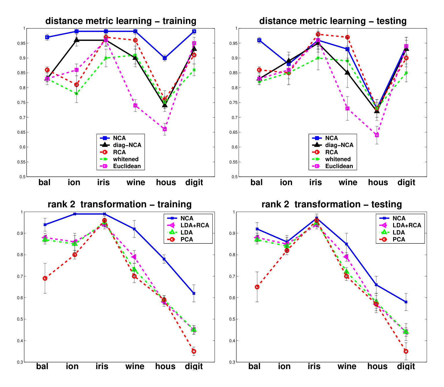
Figure 1 shows that the training and (more importantly) testing performance of NCA is consistently the same as or better than that of other Mahalanobis distance measures for KNN, despite the relative simplicity of the NCA objective function and the fact that the distance metric being learned is nothing more than a positive definite matrix $A^\top A$.

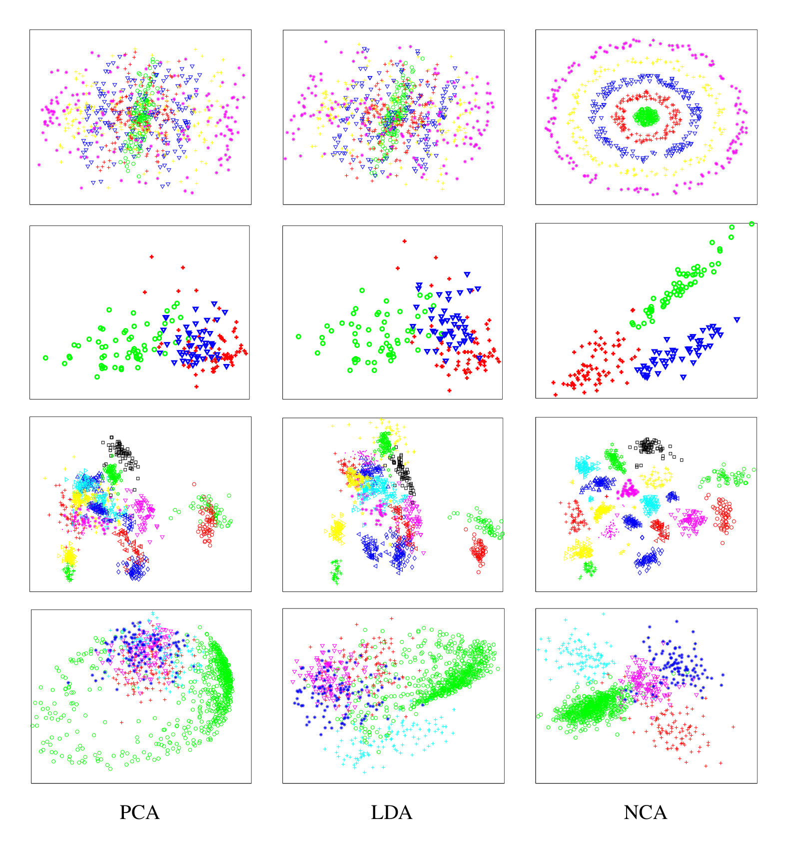
We have also investigated the use of linear dimensionality reduction using NCA (with nonsquare $A$) for visualization as well as reduced-complexity classification on several datasets. In figure 2 we show 4 examples of 2-D visualization. First, we generated a synthetic three-dimensional dataset (shown in top row of figure 2) which consists of 5 classes (shown by different colors). In two dimensions, the classes are distributed in concentric circles, while the third dimension is just Gaussian noise, uncorrelated with the other dimensions or the class label. If the noise variance is large enough, the projection found by PCA is forced to include the noise (as shown on the top left of figure 2). (A full rank Euclidean metric would also be misled by this dimension.) The classes are not convex and cannot be linearly separated, hence the results obtained from LDA will be inappropriate (as shown in figure 2). In contrast, NCA adaptively finds the best projection without assuming any parametric structure in the low dimensional representation. We have also applied NCA to the UCI “wine” dataset, which consists of 178 points labeled into 3 classes and to a database of gray-scale images of faces consisting of 18 classes (each a separate individual) and 560 dimensions (image size is $20 \times 28$). The face dataset consists of 1800 images (100 for each person). Finally, we applied our algorithm to a subset of the USPS dataset of handwritten digit images, consisting of the first five digit classes (“one” through “five”). The grayscale images were downsampled to $8 \times 8$ pixel resolution resulting in 64 dimensions.

As can be seen in figure 2 when a two-dimensional projection is used, the classes are consistently much better separated by the NCA transformation than by either PCA (which is unsupervised) or LDA (which has access to the class labels). Of course, the NCA transformation is still only a linear projection, just optimized with a cost function which explicitly encourages local separation. To further quantify the projection results we can apply a nearest-neighbor classification in the projected space. Using the same projection learned at training time, we project the training set and all future test points and perform KNN in the low-dimensional space using the Euclidean measure. The results under the PCA, LDA, LDA followed by RCA and NCA transformations (using K=1) appear in figure 1. The NCA projection consistently gives superior performance in this highly constrained low-rank KNN setting. In summary, we have found that when labeled data is available, NCA performs better both in terms of classification performance in the projected representation and in terms of visualization of class separation as compared to the standard methods of PCA and LDA.

5 Extensions to Continuous Labels and Semi-Supervised Learning

Section Summary: The core approach can be extended beyond discrete classes and linear maps by using nonlinear functions such as neural networks trained with gradient descent. For continuous targets, pairs of points are treated as soft matches whose contribution to the loss is weighted by how closely their labels agree, allowing learning even when explicit target values are unavailable and only information about which examples are nearby is given. This semi-supervised regime is illustrated by training a network on unlabeled face images whose pairs share similar pose and scale due to temporal continuity; the resulting two-dimensional embedding automatically recovers polar coordinates that represent rotation and size.

Although we have focused here on discrete classes, linear transformations and fully supervised learning, many extensions of this basic idea are possible. Clearly, a nonlinear transformation function $A(\cdot)$ could be learned using any architecture (such as a multilayer perceptron) trainable by gradient methods. Furthermore, it is possible to extend the classification framework presented above to the case of a real valued (continuous) supervision signal by defining the set of “correct matches” $C_i$ for point $i$ to be those points $j$ having similar (continuous) targets. This naturally leads to the idea of “soft matches”, in which the objective function becomes a sum over all pairs, each weighted by their agreement according to the targets. Learning under such an objective can still proceed even in settings where the targets are not explicitly provided as long as information identifying close pairs is available. Such semi-supervised tasks often arise in domains with strong spatial or temporal continuity constraints on the supervision, e.g. in a video of a person’s face we may assume that pose, and expression vary slowly in time even if no individual frames are ever labeled explicitly with numerical pose or expression values.

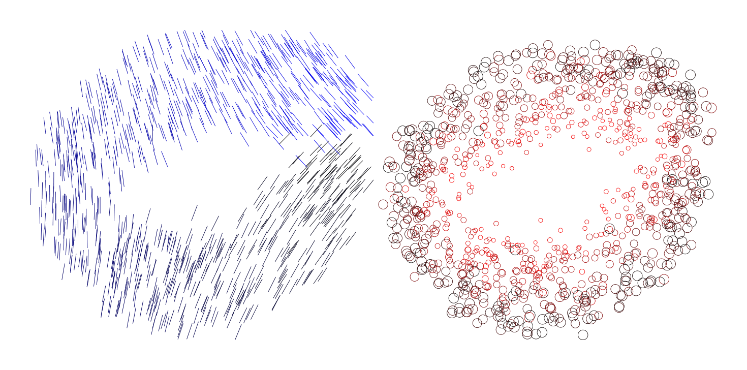
To illustrate this, we generate pairs of faces in the following way: First we choose two faces at random from the FERET-B dataset (5000 isolated faces that have a standard orientation and scale). The first face is rotated by an angle uniformly distributed between $\pm 45^\circ$ and scaled to have a height uniformly distributed between 25 and 35 pixels. The second face (which is of a different person) is given the same rotation and scaling but with Gaussian noise of $\pm 1.22^\circ$ and $\pm 1.5$ pixels. The pair is given a weight, $w_{ab}$, which is the probability density of the added noise divided by its maximum possible value. We then trained a neural network with one hidden layer of 100 logistic units to map from the $35 \times 35$ pixel intensities of a face to a point, $y$, in a 2-D output space. Backpropagation was used to minimize the cost function in Eq. 8 which encourages the faces in a pair to be placed close together:

$ \text{Cost} = - \sum_{\text{pair}(a,b)} w_{ab} \log \left( \frac{\exp(-|y_a - y_b|^2)}{\sum_{c,d} \exp(-|y_c - y_d|^2)} \right)\tag{8} $

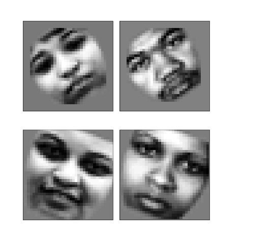
where $c$ and $d$ are indices over all of the faces, not just the ones that form a pair. Four example faces are shown to the right; horizontally the pairs agree and vertically they do not. Figure 3 above shows that the feedforward neural network discovered polar coordinates without the user having to decide how to represent scale and orientation in the output space.

6 Relationships to Other Methods and Conclusions

Section Summary: Recent approaches to learning distance measures from labeled data, including RCA and convex optimization techniques, often rely on assumptions like Gaussian class distributions or compact connected clusters that break down for complex or multimodal data. Linear discriminant analysis and its variants share similar limitations and can run into numerical instability with high-dimensional inputs, while NCA sidesteps these issues through a non-parametric linear transformation that imposes no strong assumptions on class shape or decision boundaries. The method thus unifies distance learning and dimensionality reduction in a simple yet flexible way, underscoring that linear embeddings still hold untapped potential.

Several papers recently addressed the problem of learning Mahalanobis distance functions given labeled data or at least side-information of the form of equivalence constraints. Two related methods are RCA [1] and a convex optimization based algorithm [7]. RCA is implicitly assuming a Gaussian distribution for each class (so it can be described using only the first two moments of the class-conditional distribution). Xing et. al attempt to find a transformation which minimizes all pairwise squared distances between points in the same class; this implicitly assumes that classes form a single compact connected set. For highly multimodal class distributions this cost function will be severely penalized. Lowe[6] proposed a method similar to ours but used a more limited idea for learning a nearest neighbour distance metric. In his approach, the metric is constrained to be diagonal (as well, it is somewhat redundantly parameterized), and the objective function corresponds to the average squared error between the true class distribution and the predicted distribution, which is not entirely appropriate in a more probabilistic setting.

In parallel there has been work on learning low rank transformations for fast classification and visualization. The classic LDA algorithm[3] is optimal if all class distributions are Gaussian with a single shared covariance; this assumption, however is rarely true. LDA also suffers from a small sample size problem when dealing with high-dimensional data when the within-class scatter matrix is nearly singular[2]. Recent variants of LDA (e.g. [5], [2]) make the transformation more robust to outliers and to numerical instability when not enough datapoints are available. (This problem does not exist in our method since there is no need for a matrix inversion.)

In general, there are two classes of regularization assumption that are common in linear methods for classification. The first is a strong parametric assumption about the structure of the class distributions (typically enforcing connected or even convex structure); the second is an assumption about the decision boundary (typically enforcing a hyperplane). Our method makes neither of these assumptions, relying instead on the strong regularization imposed by restricting ourselves to a linear transformation of the original inputs.

Future research on the NCA model will investigate using local estimates of $K$ as derived from the entropy of the distributions $p_{ij}$; the possible use of a stochastic classification rule at test time; and more systematic comparisons between the objective functions $f$ and $g$.

To conclude, we have introduced a novel non-parametric learning method — NCA — that handles the tasks of distance learning and dimensionality reduction in a unified manner. Although much recent effort has focused on non-linear methods, we feel that linear embedding has still not fully fulfilled its potential for either visualization or learning.

Acknowledgments

Thanks to David Heckerman and Paul Viola for suggesting that we investigate the alternative cost $g(A)$ and the case of diagonal $A$.

References

Section Summary: The references section lists seven academic papers drawn from machine learning and pattern recognition literature. They include both foundational works, such as Fisher’s 1936 paper on statistical classification, and more recent studies on distance metrics, dimensionality reduction, and face recognition algorithms. The citations range from 1936 to 2004 and appear to support technical claims made elsewhere in the document.

[1] A. Bar-Hillel, T. Hertz, N. Shental, and D. Weinshall. Learning distance functions using equivalence relation. In International Conference on Machine Learning, 2003.

[2] L. Chen, H. Liao, M. Ko, J. Lin, and G. Yu. A new lda-based face recognition system which can solve the small sample size problem. In Pattern Recognition, pages 1713–1726, 2000.

[3] R. A. Fisher. The use of multiple measurements in taxonomic problems. In Annual of Eugenic, pages 179–188, 1936.

[4] J. Friedman, J.bentley, and R. Finkel. An algorithm for finding best matches in logarithmic expected time. In ACM, 1977.

[5] Y. Koren and L. Carmel. Robust linear dimensionality reduction. In IEEE Trans. Vis. and Comp. Graph., pages 459–470, 2004.

[6] D. Lowe. Similarity metric learning for a variable kernel classifier. In Neural Computation, pages 72–85, 1995.

[7] E.P. Xing, A. Y. Ng, M.I. Jordan, and S. Russell. Distance learning metric. In Proc. of Neural Information Processing Systems, 2003.