Stop Indexing at Full Precision: Revisiting Clustering for Vector Embeddings

Leonardo Kuffo
CWI
Amsterdam, The Netherlands
[email protected]

Peter Boncz
CWI
Amsterdam, The Netherlands
[email protected]

Abstract

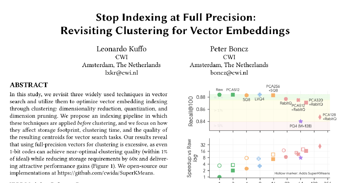
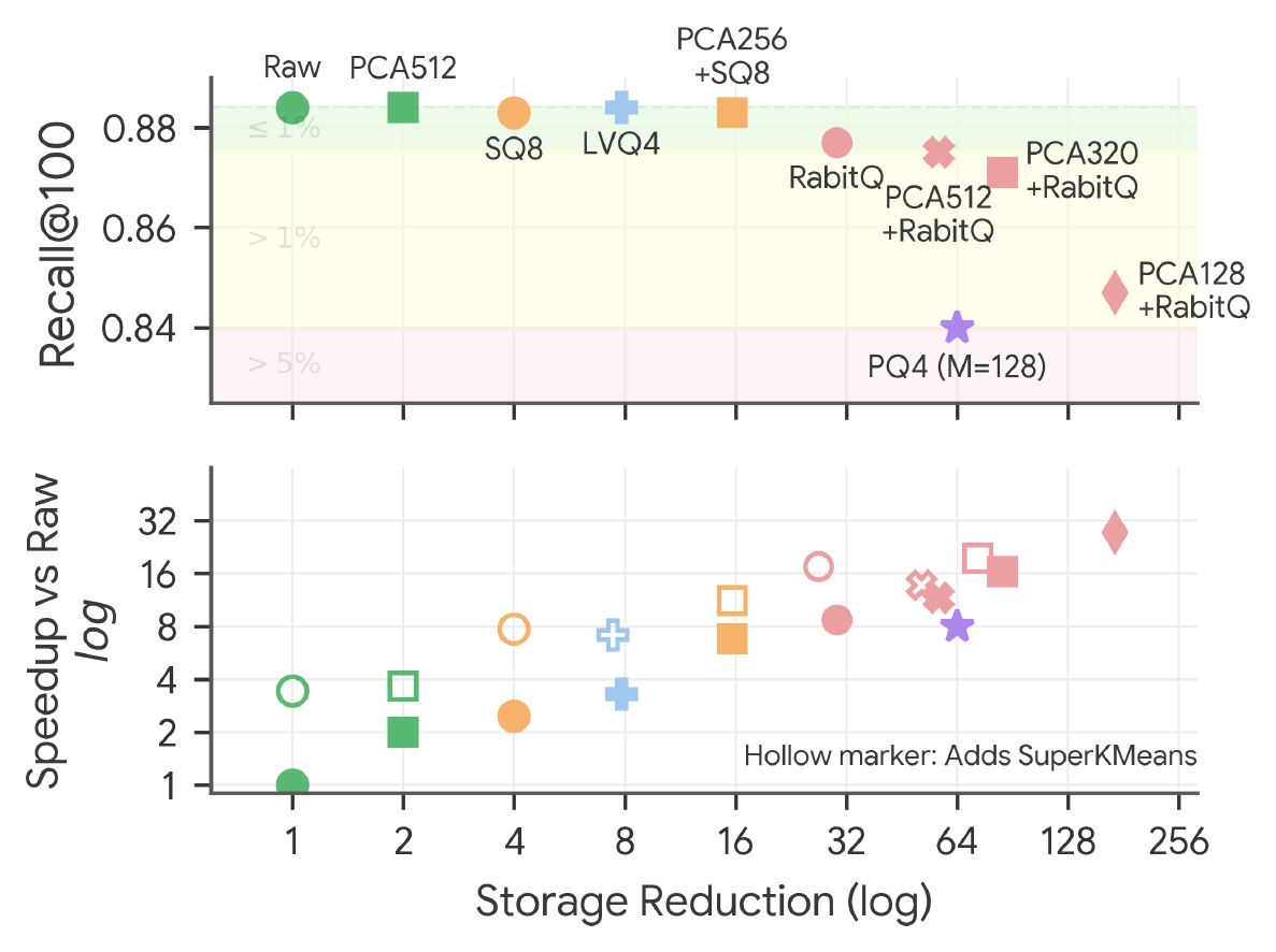
In this study, we revisit three widely used techniques in vector search and utilize them to optimize vector embedding indexing through clustering: dimensionality reduction, quantization, and dimension pruning. We propose an indexing pipeline in which these techniques are applied before clustering, and we focus on how they affect storage footprint, clustering time, and the quality of the resulting centroids for vector search tasks. Our results reveal that using full-precision vectors for clustering is excessive, as even 1-bit codes can achieve near-optimal clustering quality (within 1% of ideal) while reducing storage requirements by 60x and delivering attractive performance gains (Figure 1). We open-source our implementations at https://github.com/cwida/SuperKMeans.

Executive Summary: Clustering algorithms such as k-means are widely used to build partition-based indexes for approximate vector similarity search. These indexes group high-dimensional embeddings into clusters whose centroids guide queries toward the most promising regions of the data. However, clustering itself is a major bottleneck: it is compute- and memory-intensive, requires multiple passes over the full-precision vectors, and must complete before users can issue queries. Most production systems therefore perform clustering on full-precision data and apply compression only afterward.

This paper set out to test whether three established approximation techniques—dimensionality reduction, quantization, and dimension pruning—could be moved to the front of the pipeline and still produce centroids of comparable quality for downstream vector search. The authors evaluated combinations of PCA, Johnson-Lindenstrauss transforms, Matryoshka prefixes, scalar and product quantization at 8- and 4-bit widths, 1-bit RabitQ, and the SuperKMeans pruning method on several public embedding collections ranging from one to fifty million vectors.

The central result is that full-precision vectors are unnecessary for clustering. Applying PCA to retain 60–80 % of the variance followed by aggressive 1-bit RabitQ quantization yields centroids whose recall@100 in an IVF index stays within 1 % of the ideal full-precision baseline. The same configuration reduces the memory footprint of the clustering phase by roughly 60× and delivers substantial wall-clock speed-ups; hierarchical k-means on the compressed data can index fifty million vectors in under a minute on a single server. Storage savings and speed gains hold across multiple datasets and probing budgets, while cluster balance and within-cluster sum of squares remain acceptable.

These findings matter because vector ingestion pipelines in cloud systems are billed by the second and often must run on limited memory. Moving compression earlier eliminates repeated round-trips to raw data, lowers the hardware required for indexing, and allows the same compressed representation to serve both indexing and search. The approach also scales sub-linearly with the number of clusters, which is increasingly important as practitioners raise the number of centroids to improve search latency.

The authors recommend that systems already using a given quantization or projection scheme for search should apply the same encoding before clustering. When near-optimal quality is required, LVQ at 4 bits with 80 % PCA variance offers the safest trade-off; when modest quality loss is acceptable, RabitQ plus SuperKMeans provides the largest speed and storage gains. Hierarchical k-means or modest sampling can be layered on top for very large collections. The main limitations are that the study used only embedding datasets and CPU hardware, and that some quantization schemes still benefit from a final refinement pass on raw vectors to restore perfect cluster balance. The open-source implementation allows practitioners to validate these trade-offs on their own data before committing to production changes.

1. Introduction

Section Summary: Clustering algorithms like k-means are commonly used to organize large collections of high-dimensional vectors for fast similarity searches, by grouping them around representative centroids that guide queries to the most relevant areas and avoid scanning the entire dataset. However, the clustering step itself is computationally demanding, requires repeated full passes over the raw data, and creates a major bottleneck during index construction, unlike the more efficient pruning done at search time. This work shows that applying dimensionality reduction, quantization, and pruning techniques before clustering can deliver near-optimal results with far less memory and time, achieving up to 60x storage savings while maintaining index quality.

Nowadays, clustering algorithms (e.g., $k$-means [1]) are utilized in approximate vector similarity search (VSS) to index large collections of high-dimensional vectors [2, 3, 4, 5, 6, 7, 8, 9, 10, 11, 12, 13, 14]. VSS consists of finding the vectors in a collection that are the most similar to a given query vector, based on a distance or similarity metric. When a vector collection is indexed using clustering, the resulting centroids act as entry points to guide queries to the clusters that are most likely to contain their nearest neighbors. Thus, reducing search latency by avoiding accessing the majority of the collection. This indexing method remains a popular option across vector systems due to its scalability and advantages in data management tasks compared to other index families, such as graph-based ones [10, 2, 15, 16, 7, 3, 17, 18].

{width=60%}

Clustering poses major challenges compared to VSS. First, it is not only memory-bound but also heavily compute-bound [19, 11, 20, 21]. Furthermore, it requires accessing the entire collection of raw vectors multiple times, whereas VSS prunes most of the vector collection on every query. As a result, clustering remains a critical step that bottlenecks user queries until the index is built. Despite this, most research efforts focus on search algorithms, with few addressing vector indexing via clustering [20, 11, 22, 23, 24, 21].

In this work, we revisit three widely used techniques for vector search and use them for vector indexing via clustering: dimensionality reduction (JLT [25, 26, 22], PCA [27, 28, 29, 30, 24], Matryoshka vectors [31]), quantization (SQ [8], LVQ [32], RabitQ [33, 6, 9], PQ [34, 35]), and dimension pruning [36, 37, 38, 39, 40, 13]. We propose an indexing pipeline that applies these techniques before clustering, resulting in attractive performance gains and storage reductions without sacrificing index quality. Our pipeline design differs from most systems, where clustering uses full-precision vectors and quantization occurs only after clustering [41, 42, 8, 9].

Our results show that using full-precision vectors for clustering is excessive, as even using 1-bit RabitQ codes of PCA-projected vectors achieves near-optimal clustering quality (less than 1% degradation) with 60x storage reduction. As part of our contributions, we adapt dimension-pruning techniques (SuperKMeans [11], ADSampling [39]) to integrate with quantization schemes to further accelerate clustering without sacrificing quality. Finally, we explore several design decisions across the indexing pipeline that affect performance and the quality of clusters for vector search tasks.

2. Preliminaries

Section Summary: Vector search systems often rely on approximate nearest-neighbor methods that organize large collections of vectors into clusters so that only a small subset needs checking for each query. These clusters are typically built with a simple k-means procedure that repeatedly assigns every vector to the nearest center using fast matrix multiplications and then updates the centers by averaging assigned points, usually running for only a few iterations. Although clustering is essential for creating practical indexes, it remains a major performance bottleneck and has received far less optimization attention than the search step itself.

2.1 Vector Search

Nearest Neighbor Search (NNS) consists of finding the closest vectors in a collection to a given query vector, based on a distance or similarity metric. Finding exact answers is often impractical due to the large compute and storage requirements. However, modern applications such as RAG and Recommender Systems powered by NNS typically do not require exact answers as approximate answers are "good enough". This is known as Approximate Nearest Neighbor Search (ANNS), or Vector Similarity Search (VSS). The approximate nature of VSS enables the use of techniques that reduce storage and compute requirements during query time, such as quantization [8, 32, 35, 33, 6, 43], dimension pruning [37, 38, 39, 44], and dimensionality reduction [31, 25, 27, 30, 45].

These techniques are usually combined with approximate indexes [46, 35, 6, 4] that guide queries toward the most promising vectors in the collection. Among vector indexes, two main families exist: partition-based [4, 3, 47, 2, 48, 35, 49] and graph-based [50, 51, 52, 53, 46]. While graph-based indexes can answer queries with fewer distance comparisons than partition-based indexes [54], they take a considerably higher amount of time to build [50, 11, 48, 17]. Furthermore, they introduce additional complexity in data management tasks, such as ingestion and updates [55, 16, 49], as well as when combining VSS with traditional SQL-like filtering [56, 57, 58]. This makes partition-based indexes an attractive option for large collections and distributed or cloud environments [7, 59, 18, 3, 2, 12].

2.2 The Role of Clustering in Vector Search

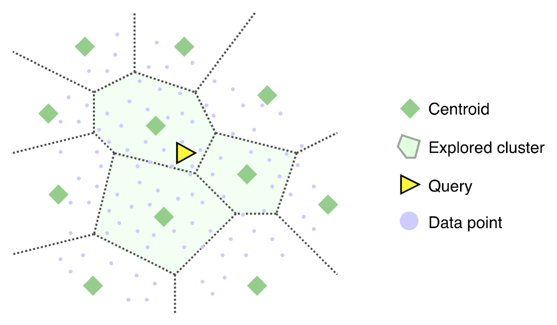
Partition-based indexes, such as the widely used Inverted-Files (IVF), organize a collection of vectors into clusters through clustering methods like $k$-means [8, 4, 3]. During query time, the distance metric is first evaluated between the query $q$ and the centroids $Y$. Then, the vectors within the nearest clusters are chosen for evaluation (Figure 2). By adjusting the number of explored clusters, one can balance search speed with quality [8, 42]. Typically, the number of centroids is set around $\sqrt{N}$ [8, 42], resulting in higher $k$ values compared to other use cases of clustering [60, 61, 62].

Despite clustering being orders of magnitude faster than graph-index construction, it remains a crucial bottleneck, as users experience degraded performance or are unable to query the collection until an index is built [17]. Additionally, the clustering of vector embeddings introduces several challenges compared to VSS. First, it requires multiple accesses to the entire vector collection (or a large subsample [11, 22]), whereas vector search typically accesses only portions of a collection with each query. Second, unlike vector search, which is mostly data-access bound [19], clustering is also heavily compute-bound due to the higher number of computations needed. On top of that, the increasing demand for vectors as first-class citizens in database systems has created new scenarios in which low-latency, low-memory indexing is essential. For instance, in a situation where an attribute-based filter is applied to a vector column [58], with the resulting vectors then utilized to perform a similarity codewordJOIN [63] with a different vector column from another table, the ability to create an index on the fly could enhance the performance of the similarity codewordJOIN operator if it can be created quickly enough.

{width=60%}

2.3 Clustering in Vector Systems

The implementation of clustering found in vector systems (e.g., cuVS [64], FAISS [8], Milvus [42], VectorChord [22], Vortex [65], LanceDB [41], Elastic [23]) follows a Lloyd $k$-means algorithm [1] or a hierarchical variant of it. In brief, $k$-means follows these steps:

STEP 1. Centroids Initialization: Centroids are initialized by randomly sampling $k$ vectors from the collection [66]. More sophisticated initializations, such as $k$-means++ [61], have proven ineffective for vector embedding datasets due to their marginal improvements while incurring substantially higher runtime [11].

STEP 2. Determining Assignments: Assignments are determined using a distance metric that identifies which point $x$ in the collection $X$ is closest to which centroid $y$ of $Y$. The L2 Euclidean distance is the most commonly used. This step is the main bottleneck of clustering, as it requires computing pairwise distances between every $x$ in $X$ and every $y$ in $Y$. The most efficient way to do this is through a General Matrix Multiplication (GEMM) of the data points and centroids ($\colorbox{lightpeach}{(\displaystyle X \boldsymbol{\cdot} Y)}$). GEMM routines are highly efficient due to their optimized data access patterns, vectorization (SIMD), efficient cache usage, and multi-threading.

STEP 3. Updating Centroids: Centroids are updated by averaging every vector $x$ assigned to them. When centroids have zero assignments, it is beneficial to split large clusters to achieve a more balanced distribution of points across clusters—a desirable characteristic for partition-based indexes used in VSS [2, 4, 67].

Termination Conditions and Final Assignments: The algorithm terminates after a predetermined number of iterations of STEPS 2 and 3, typically ranging from 5 to 10 for vector embedding datasets [11]. Then, STEP 2 is executed once more to obtain the final assignments of each point to its nearest centroid.

2.4 Efforts to Optimize Vector Clustering

Research on optimizing clustering of vector embeddings has received far less attention than vector search algorithms. Nevertheless, a few techniques tailored for vector search have seen success when applied to vector clustering [22, 11, 23, 20, 24].

Dimensionality reduction aims to represent vectors in a lower-dimensional space, thereby reducing memory footprint and compute requirements [28, 45, 30]. VectorChord employs a Johnson– Lindenstrauss Transform (JLT) [25] to reduce the dimensionality of the raw vectors before clustering [22]. This reduces the memory footprint of clustering while providing performance gains from fewer computations [68, 25, 22]. LindormVector [24] accomplishes the same goal with a PCA (Principal Component Analysis) projection that concentrates the vectors' energy in the leading dimensions. More recently, embedding models have been trained to generate Matryoshka embeddings [31], which already concentrate energy in the front dimensions. However, the impact of dimensionality reduction on clustering quality has not been thoroughly studied.

Quantization techniques aim to represent each dimension of a vector, or a group of dimensions, with smaller codes while minimizing distortion in the distance metric between points [33, 32, 69]. PQk-means is one of the few studies that use quantization prior to clustering [20]. PQk-means encodes vectors using Product Quantization [35], effectively reducing memory usage and accelerating distance calculations, albeit at the cost of clustering quality. More recent quantization techniques, such as LVQ [32, 70] and RabitQ [33, 6, 46], have not been used for vector clustering.

Dimension pruning aims to break off distance computations when the distance metric has enough resolution to determine that a point will not be the nearest neighbor of a query [39, 36, 40, 71, 37, 38]. SuperKMeans integrates dimension pruning into vector clustering by interleaving GEMM routines and pruning kernels, achieving substantial speedups without sacrificing clustering quality [11]. However, it remains unclear whether SuperKMeans can be combined with the previously mentioned techniques.

The impact of approximations on clustering quality has not been thoroughly studied. In most clustering pipelines, vectors are indexed at full precision (codewordfloat32, codewordfloat16) before being projected into a smaller $d$-dimensional space [28, 29, 45, 30], quantized [9, 32, 28], and materialized in the index data structure. In this study, we show that approximation techniques can be applied first in the indexing pipeline, saving several round trips to the raw data, reducing memory footprint during clustering, and delivering attractive performance gains, all while mostly preserving clustering quality.

2.5 Keys for the Performance of Clustering

GEMM routines for codewordfloat32 are the fuel for high-performance clustering, having undergone decades of optimization. Consequently, clustering speed improves with dimensionality reduction, as $d$ decreases while maintaining codewordfloat32 as the data type. Dimension pruning further improves speed by reducing the number of distance calculations. However, the performance of clustering becomes more nuanced when working with quantized vectors. Ideally, the quantization method should facilitate efficient many-to-many distance calculations that leverage modern CPU capabilities for processing smaller data types, such as 8-bit integers. Nonetheless, the performance benefits depend on the availability of SIMD [19, 72, 73, 74, 75] or specialized hardware (e.g., Intel's AMX [76, 77]) that can efficiently handle 8-bit data types.

{width=70%}

2.6 The Resilience of Clustering

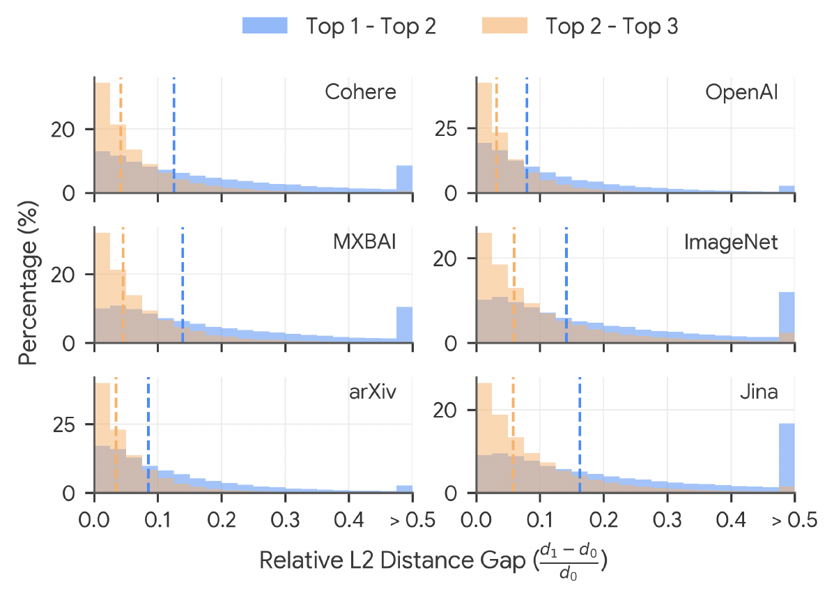
The assignment step in the clustering process (STEP 2) is effectively a series of top-1 NNS queries with roles reversed: the vector collection acts as the queries, while the centroids become the vector collection to query. Figure 3 shows the distribution of the relative L2 distance gap between vectors and their nearest centroids across several vector embedding datasets. Notably, the gap between the top-1 and top-2 nearest centroids (in blue) is 2-3x larger than that of the next neighboring centroids (top-2 and top-3, in yellow), making the top-1 centroid distinctly identifiable. In contrast, the 2nd and 3rd nearest centroids are typically close to one another. This phenomenon makes vector clustering far more resilient to approximation techniques compared to vector search, as errors introduced by methods such as quantization are less likely to affect the correct assignment to the closest centroid [78]. This observation raises the question: To what extent can techniques utilized in vector search be applied to vector clustering? In the remainder of this study, we empirically address this question by examining the effects of several techniques (and their combinations) on the quality of clustering.

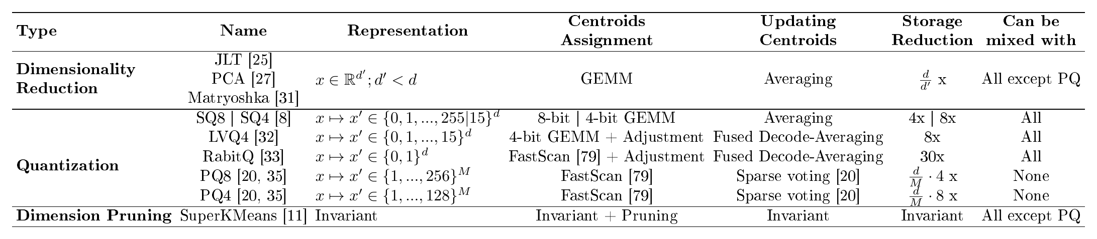
::: {caption="Table 1: Techniques used in our clustering pipeline."}

:::

3. Our Pipeline: Approximate First, then Cluster

Section Summary: The proposed pipeline performs dimensionality reduction and quantization on vectors before any clustering step, then applies dimension pruning during clustering itself to limit expensive distance calculations. This reverses the usual approach of clustering full-precision data first and quantizing only afterward. The section explains how standard quantization methods such as SQ, LVQ, and RabitQ are adapted so that both distance computations and centroid updates can be carried out efficiently in the reduced, quantized domain.

We propose an indexing pipeline (shown in Figure 4) where dimensionality reduction and quantization occur before clustering, and dimension pruning is used during clustering to reduce the number of distance calculations. This design differs from most systems, which typically use full-precision vectors for clustering and apply quantization only after the clustering stage [41, 42, 8, 9]. Table 1 presents the techniques we have chosen for our evaluation. Next, we describe how we adapted these techniques for clustering.

3.1 Adapting Techniques for Vector Clustering

SQ8 and SQ4: In SQ, each value $x_i$ of a vector $x$ is encoded with a global bias $b = v_{min}$, and a global scaling factor $s = \frac{v_{max} - b}{c_{max}}$, where $c_{max} = 2^B -1 $ and $B$ is the quantization bit-width. Each quantized code $\bar{x}_i$ is defined as $\bar{x}i = \operatorname{clip} \left(\left\lfloor \frac{x_i - b}{s}\right\rceil, 0, c{max} \right) $, and reconstructed as: $x_i \approx (\bar{x}_i \cdot s) + b$. Since all vectors are transformed with the same parameters, distance computations can be performed directly in the quantized domain using integer arithmetic, leveraging 8- and 4-bit GEMM routines [72, 80]. Finally, updating centroids can be done by averaging each dimension, also in the quantized domain.

LVQ4: In LVQ [32], each value $x_i$ of a vector $x$ is encoded with a per-vector bias $b_x = x_{min}$, and scale $s_x = \frac{x_{max} - b_x}{c_{max}}; c_{max} = 2^B-1$. Each quantized code $\bar{x}_i$ is defined as $\bar{x}i = \operatorname{clip} \left(\left\lfloor \frac{x_i - b_x}{s_x}\right\rceil, 0, c{max} \right) $, and reconstructed as: $x_i \approx (s_x \cdot \bar{x}_i) + b_x$. Since each vector has a different $s$ and $b$, the codes cannot be used directly for distance calculations. To solve this, LVQ proposes fusing reconstruction of codewordfloat32 values with distance calculations. However, by doing so we lose the benefits of using a smaller data type. Furthermore, in many-to-many distance calculations, the reconstruction step is performed multiple times for the same vectors, which hurts efficiency. Hereby, we rewrite the L2 distance $||x - y||^2$ as:

$ \begin{aligned}||x - y||^2 & \approx \sum_{i}^{d} ((s_x \bar{x}{i} + b_x) - (s_y \bar{y}{i} + b_y))^2\& \approx s_x^2 \sum_{i}^{d} \bar{x}{i}^2 + s_y^2 \sum{i}^{d} \bar{y}{i}^2 - 2 s_x s_y \colorbox{lightpeach}{(\displaystyle \langle{\bar{x}, \bar{y}} \rangle)}\& ;;;; + 2(b_x - b_y) (s_x \sum{i}^{d} \bar{x}{i} - s_y \sum{i}^{d} \bar{y}_{i}) + d (b_x - b_y)^2\end{aligned}\tag{1} $

Collecting constant $x$-only terms into $N_x = s_x^2 \Sigma \bar{x}{i}^2 + 2 b_x s_x \Sigma \bar{x}{i} + d b_x^2$, and $y$-only terms into $N_y = s_y^2 \Sigma \bar{y}{i}^2 + 2 b_y s_y \Sigma \bar{y}{i} + d b_y^2$, and defining $A_x = s_x \Sigma \bar{x} + d b_x$:

$ \begin{aligned} ||x - y||^2 \approx N_x + N_y - 2\bigl(s_x \cdot s_y \cdot \colorbox{lightpeach}{(\displaystyle \langle \bar{x}, \bar{y} \rangle)} + b_y \cdot A_x + b_x \cdot s_y \Sigma \bar{y}_{i}\bigr) \end{aligned}\tag{2} $

This derivation allows us to use 4-bit GEMM kernels to compute the highlighted term. The final distances require additional scalar operations, from which $N_x$ and $A_x$ terms can be cached across $k$-means iterations, while $N_y$ can be computed once at the start of each iteration. Finally, when updating centroids, we cannot solely use LVQ codes, as averaging them is undefined. Thus, we fuse the decoding and averaging of the LVQ codes of the centroid assignments and re-encode the resulting centroids.

RabitQ: In RabitQ, each vector is centered, normalized to the unit sphere, and randomly rotated. Then, each dimension is quantized to 1-bit by only preserving their sign. Due to the properties of a random rotation, this quantized vector $\bar{x}$ of signs lives in the codebook ${+1/\sqrt{d}, , -1/\sqrt{d}}^d$. RabitQ then provides an unbiased estimator of L2 distances and guarantees that the estimator has an asymptotically optimal error bound [33]. Let $x_r$ be a raw data vector and $y_r$ be a raw query, normalized based on a vector $m$ (i.e., the dataset means). Now, let $x := \frac{x_r - m}{||x_r - m||}$ and $y := \frac{y_r - m}{||y_r - m||}$. The L2 distance between $x_r$ and $y_r$ can be expressed as:

$ \begin{aligned}||x_r - y_r||^2 & = ||(x_r - m) - (y_r - m)||^2\& = ||x_r - m||^2 + ||y_r - m ||^2\& ;;;; - 2 \cdot ||x_r - m|| \cdot ||y_r - m|| \cdot \colorbox{softblue}{(\displaystyle \langle x, y \rangle)}\end{aligned}\tag{3} $

From which $||x_r -m||$ can be computed and cached in the first iteration of $k$-means and $||y_r - m||$ can be precomputed once per centroid, and thus, is amortized by all the pairwise distance calculations. For the term, $\displaystyle \langle x, y \rangle$ , RabitQ derives an unbiased estimator. Let $\bar{x}$ denote the 1-bit quantized version of $x$, then: $\langle x, y \rangle \approx \frac{\langle \bar{x}, y \rangle} {\langle \bar{x}, x \rangle} $, where $\langle \bar{x}, x \rangle$ is the cosine between the original and quantized unit vector, precomputed and stored per data point. Substituting into Equation 3, and recalling that $y:= \frac{y_r - m}{||y_r - m||}$, then we derive:

$ ||x_r - y_r||^2 \approx ||x_r - m||^2 + ||y_r - m||^2

• 2 \cdot \colorbox{softpink}{(\displaystyle \frac{||x_r - m||}{\langle \bar{x}, x \rangle})} \cdot \colorbox{softblue}{(\displaystyle \langle \bar{x}, , y_r - m \rangle)}\tag{4} $

The scalar factors $||x_r - m||^2$ and $\colorbox{softpink}{(\displaystyle ||x_r - m||/\langle \bar{x}, x \rangle)}$ depend only on the data points and can be cached across $k$-means iterations, while $||y_r - m||^2$ can be computed once at the start of each iteration. In RabitQ, the centered residual vector $y_r - m$ is quantized with SQ4 ($\bar{y}$), with scale $s$ and bias $b$. Then, expanding the SQ4 reconstruction $ (y_r - m)_i \approx \bar{y}_i \cdot s + b$ and reconstructing the codebook with the stored bits $\bar{x}_i \in {0, 1}$, so that each codebook entry is $(2\bar{x}_i- 1)/\sqrt{d}$, yields the following estimator for $\colorbox{softblue}{(\displaystyle \langle \bar{x}, , y_r - m \rangle)}$:

$ \begin{aligned} \langle \bar{x}, \bar{y} \rangle & \approx \frac{1}{\sqrt{d}} \sum_{i}^{d} (2\bar{x}{i} - 1)(b + \bar{y}i \cdot s) \ & \approx \frac{1}{\sqrt{d}} \Big[s \cdot \Big(2 \colorbox{lightpeach}{(\displaystyle \sum{i}^{d} \bar{x}{i} \cdot \bar{y}{i})} - \sum{i}^{d} \bar{y}i \Big) + b \cdot \Big(\Big(2\sum{i}^{d}\bar{x_i}\Big) - d \Big) \Big] \ \end{aligned}\tag{5} $

The challenge in computing the highlighted term arises from operand asymmetry: $\bar{x}$ is binary while $\bar{y}$ is SQ4. This computation can be done efficiently using in-register 4-bit lookup tables with the codewordPSHUFB [81] instruction, which allows for 32 lookups at a time. This method is known as FastScan [79]. The lookup tables can be built on the fly during each iteration of $k$-means. The other terms are scalar operations performed once per distance calculation. In our vector clustering pipeline, we encode data points (which act as queries) with 1-bit RabitQ and the centroids with SQ4. We took this approach because the data points bound the memory footprint of clustering. Finally, when updating centroids, we fuse the decoding of RabitQ codes with the averaging of centroid assignments, then re-encode the resulting centroid with SQ4. The decoding of RabitQ codes reconstructs each coordinate $x_{r_i}$ as $x_{r_i} \approx m_i + \frac{1}{\sqrt{d}} \cdot \colorbox{softpink}{(\displaystyle ||x_r - m||/\langle \bar{x}, x \rangle)} \cdot (2\bar{x}_i - 1); ;; \bar{x}_i \in {0, 1}$.

PQ8 and PQ4: In PQ [35], the dimensions are divided into $M$, $\frac{d}{M}$ -dimensional subspaces. Each group $M$ is represented with an 8- or 4-bit code from a codebook trained for each subspace. PQ8 allows for 256 different codes, while PQ4 allows for 16 codes. These codes map to representative centroids in each subspace. For encoding a vector $x$, each dimension group is assigned the closest centroid code from the codebook of each subspace. As both data and centroids are product-quantized, we use Symmetric Distance Comparisons (code-to-code) to compute assignments. PQ4 can do this efficiently with FastScan [79], while PQ8 uses scalar lookups as its 8-bit codes are incompatible with the codewordPSHUFB instruction. Finally, when updating centroids, we adopt the sparse voting mechanism introduced in PQk-means [20].

SuperKMeans accelerates distance calculations during centroid assignment by interleaving GEMM routines for the front $d'$ dimensions (set to 12.5% of $d$) and using progressive-pruning kernels every 64 dimensions on the surviving candidates [11]. A random orthogonal rotation is required for pruning. This transformation distributes the variance more evenly across all dimensions while preserving the L2 distances between vectors, enabling reliable pruning using ADSampling [39]. In SQ8 and SQ4, SuperKMeans is extended by replacing the codewordfloat32 GEMM with 8- and 4-bit GEMMs. However, SuperKMeans encounters limitations with LVQ and RabitQ because it requires L2 distances at $d'$, where $d' < d$. Both LVQ and RabitQ derivations (Equations 2 and 3) can be used with $d'$, as the L2 distance can be decomposed as $||x-y||^2 = ||x'-y'||^2 + ||x''-y''||^2$, where $x'$ refers to the front $d'$ dimensions of $x$, and $x''$ to the remaining ones. However, this incurs storage overhead for the adjustment factors needed per dimension segment, as well as the additional overhead of floating-point operations. Hereby, for LVQ4 and RabitQ, we use only 2 pruning checkpoints at 12.5% and 25% of $d$. For progressive pruning to take place, efficient 1-to-1 distance kernels are also necessary. In SQ8, SQ4, and LVQ4, we use 8- and 4-bit L2 distance kernels [72]. In RabitQ, we use the codewordPOPCNT-per-bitplane approach described in [33].

The Johnson–Lindenstrauss Transform (JLT) projects vectors to a lower $d'$ while preserving pairwise distances between the points [26, 25]. Principal Component Analysis (PCA) projects vectors into a lower $d'$ while preserving global variance and concentrating the energy of the vectors in the front dimensions. Matryoshka vectors are produced by embedding models that already concentrate the energy in the front dimensions [31]. These techniques do not need extra engineering to be integrated in the clustering pipeline, as vectors remain in the codewordfloat32 domain.

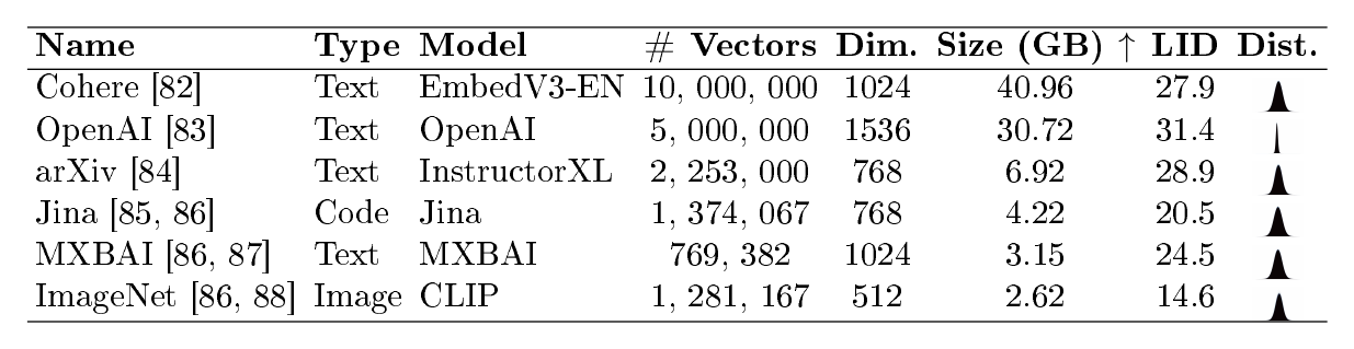
::: {caption="Table 2: Vector embedding datasets used for evaluation"}

:::

4. Evaluation

Section Summary: The evaluation tests the indexing pipeline on multiple vector datasets by measuring three main factors: how well the resulting cluster centroids support accurate vector search via recall metrics in IVF indexes, the reduction in storage needed during clustering, and the overall runtime for repeated k-means iterations. Quality is further checked using cluster compactness scores and by comparing quantized approaches against raw vectors under different search probing levels. Results highlight that select quantization methods combined with acceleration techniques deliver near-ideal search performance alongside major gains in storage and speed.

We experimentally evaluate our indexing pipeline using the vector embedding datasets presented in Table 2. Our evaluation focuses on three aspects: (i) clustering quality, (ii) storage reduction, and (iii) clustering speed. For clustering quality, we assess how well the generated centroids perform in vector search tasks when used as an entry point for an IVF index. To quantify this, we use the recall@k metric together with the number of vectors explored during search, which serves as a proxy for the amount of distance computation required. Recall@k measures the proportion of the true nearest neighbors (i.e., the ground truth) that are retrieved among the top- $k$ results. In our evaluation, we retrieve the top 100 neighbors (i.e., recall@100). In IVF indexes, recall can be tuned by varying the number of clusters probed during search. We report results for two probing configurations that correspond to exploring 1% and 3% of the available clusters. For a given recall level, exploring fewer vectors is preferable as it indicates that the search requires fewer distance computations.

Additionally, we record the within-cluster sum of squares (WCSS), which measures the compactness of clusters by summing the squared distances of each point to its centroid (lower is better). Regarding storage reduction, we report the reduction in storage required to perform the clustering iterations. Finally, in terms of clustering speed, we measure the end-to-end runtime of our clustering pipeline over 10 iterations of $k$-means, setting the number of clusters to $4\sqrt{N}$ [8, 42], where $N$ is the number of vectors in the collection.

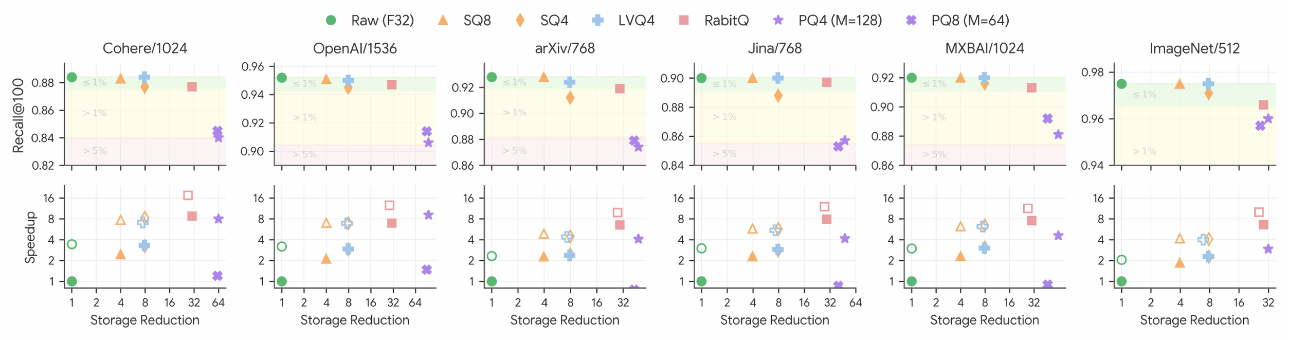
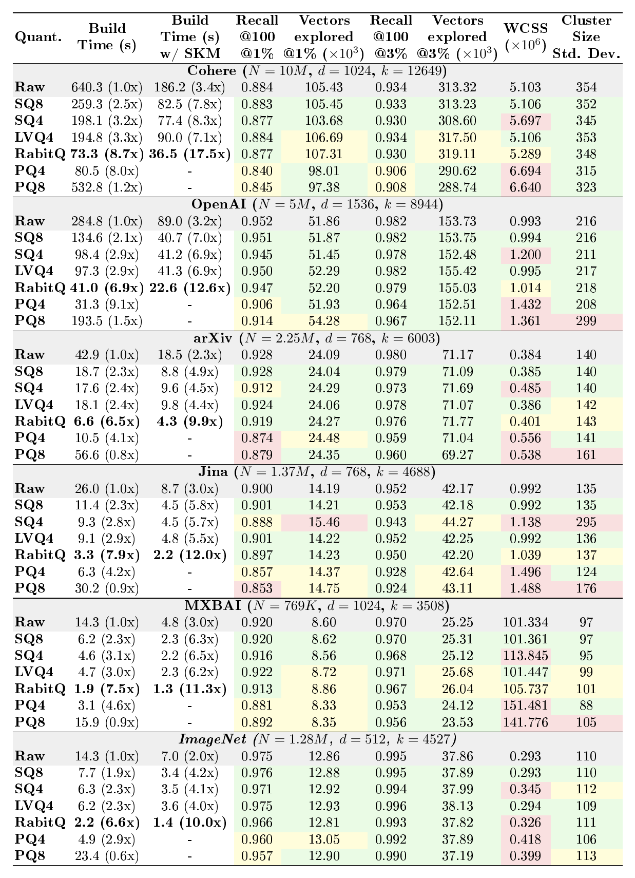
::: {caption="Table 3: Quality of the generated centroids for VSS tasks when clustering quantized vectors. To measure recall, we do top-100 IVF index searches by probing 1% and 3% of the clusters. Color coding is the same as in Table 3."}

:::

Index Materialization: The last step of our pipeline materializes the index to be used for VSS. Notably, the same representations can be used for both VSS and clustering, which avoids a round-trip to the raw vectors during index materialization. Recent studies have proposed vector indexes that utilize not only quantization but also dimensionality reduction [30, 28, 29, 45], aligning with the principles of our pipeline. To ensure a fair comparison across techniques, we compute the recall@k based on cluster membership. In other words, we assume that the vectors within the probed clusters are ranked correctly. This helps us circumvent artifacts introduced by VSS pipelines, such as re-ranking. Finally, we materialize the trained centroids for the IVF index as codewordfloat32 vectors. Unless stated otherwise, these centroids are computed solely from the reconstruction of the quantized codes of the trained centroids.

Hardware and Software: We used an AMD Zen 5 EPYC 9R45 CPU (4.5 GHz) with 256GB of RAM and 32 cores (codewordr8a.8xlarge in AWS). Our implementations extend the C++ SuperKMeans codebase [89]. We use 8- and 4-bit GEMM kernels found in the NumKong library [72] and codewordfloat32 GEMM kernels from OpenBLAS [90]. Our experiments use all the available cores.

4.1 Quantization Techniques

Table 3 (top) shows the quality of the resulting centroids for vector search tasks based on the recall they yield when used as entry points for an IVF index and probing 1% of clusters. Table 3 presents these results in detail, reporting several metrics that characterize clustering quality. SQ8 always achieves a clustering quality on-par with using raw codewordfloat32 vectors in all aspects, while providing 4x storage reduction and up to 8x speedups when paired with SuperKMeans (bottom of Table 3). LVQ4 and RabitQ achieve near-optimal clustering quality (with no more than 1% difference in recall) with 8x and 30x storage reduction, resp., while mostly maintaining cluster balance and providing significant speedups. RabitQ results in a slightly higher imbalance in cluster size. However, it provides up to 17x acceleration when paired with SuperKMeans' pruning, where the additional metadata to use SuperKMeans degrades storage reduction by around 10%. Finally, LVQ4 outperforms SQ4 in terms of clustering quality, despite both achieving the same level of storage reduction.

::: {caption="Table 4: Profiling of clustering in the Cohere dataset. The additional work of quantization methods (encoding and precomputing terms) is negligible, except on PQ4 and PQ8. The phases of SuperKMeans (SKM) are broken down."}

:::

On the other hand, PQ vectors provide the highest storage reduction but compromise clustering quality, affecting both recall and the balance of clusters. PQ struggles with clustering quality because it builds a global codebook from raw vectors, whereas PQ is typically applied to the residuals after clustering, allowing vectors to be centered around the clusters' means [8]. A way to improve the quality of PQ-based clustering is to use the raw vectors to update the centroids during the final $k$-means iteration. This brings the WCSS into the yellow zone, improving recall from 0.84 to 0.85 in the Cohere dataset, albeit at the cost of accessing the raw vectors.

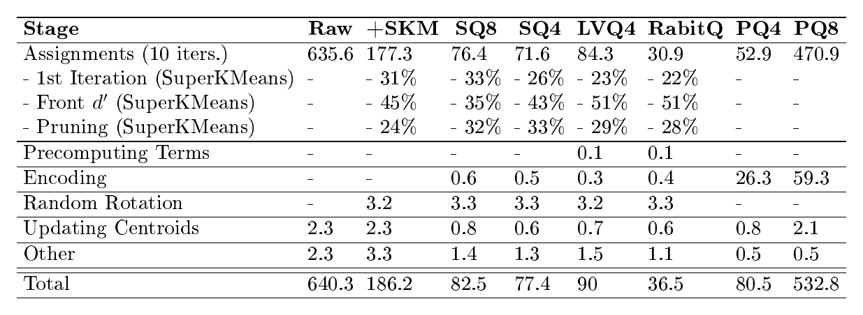
Table 4 breaks down the clustering time into different phases. All techniques, except for PQ4 and PQ8, use SuperKMeans. Notably, the time spent on encoding and precomputing constant terms in SQ, LVQ, and RabitQ is negligible. In contrast, encoding consumes a significant portion of PQ's runtime, limiting its speedup. Finally, in RabitQ and LVQ, a considerable amount of time during the assignment step is consumed by the overhead of computing partial L2 distances of the front $d'$ dimensions.

Closing RabitQ's Gap in Balance: Despite RabitQ achieving exceptional end-to-end recall, the balance of clusters is negatively impacted. Further inspection reveals that when clustering RabitQ codes, outer clusters covering the periphery of the data distribution bleed boundary points into denser in-distribution clusters–explaining the higher number of vectors explored. These outer cluster centroids are the furthest from the dataset mean ($m$ in Equation 4), which is also the root of the issue. Recall that the decoding of RabitQ codes reconstructs each coordinate $x_{r_i}$ as $x_{r_i} \approx m_i + \frac{1}{\sqrt{d}} \cdot \colorbox{softpink}{(\displaystyle ||x_r - m||/\langle \bar{x}, x \rangle)} \cdot (2\bar{x}_i - 1); ;; \bar{x}_i \in {0, 1}$. Hereby, the decoded residual sits on the sphere of radius $\displaystyle ||x_r - m||/\langle \bar{x}, x \rangle$ around $m$. By Cauchy–Schwarz, $||x_r - m||_1 \le \sqrt{d} ; ||x_r - m||$, so this radius is always at least $||x_r - m||$. Consequently, each RabitQ-decoded vector has a systematic outward reconstruction bias from the dataset mean. When these decoded vectors are averaged to form a centroid, the bias largely cancels for inner clusters (whose constituent sign patterns are diverse) but survives for peripheral clusters (whose vectors' sign patterns are highly aligned). The result is that peripheral cluster centroids are reconstructed less precisely than central ones, overshooting outward. A simple way to counteract this effect is to use the raw vectors in the last iteration to update the centroids. This brings RabitQ clusters into the green zone across all metrics, albeit at the cost of accessing the raw vectors, which may be unfeasible if they reside in a slower storage unit.

4.2 Dimensionality Reduction Techniques

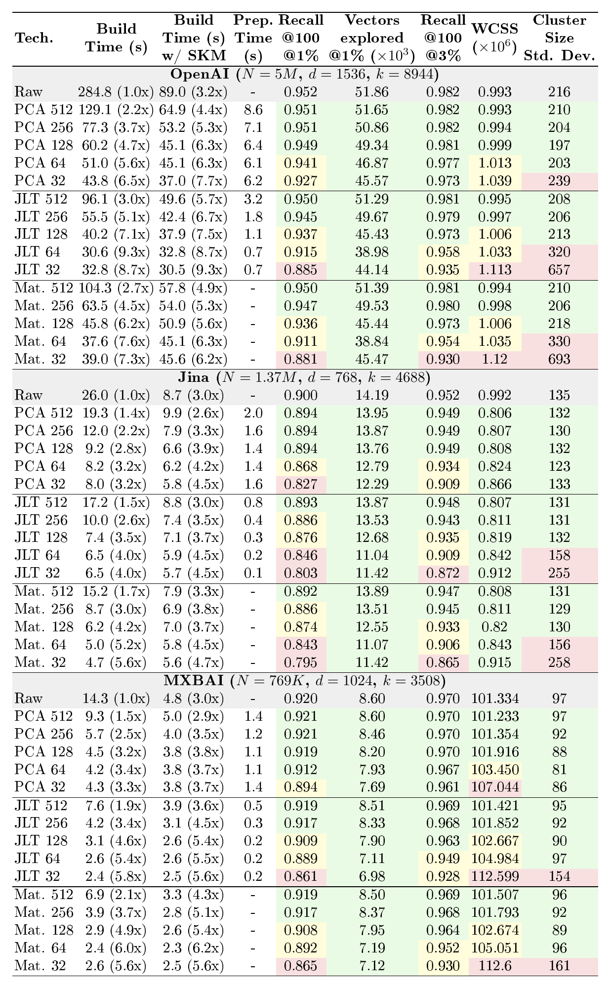
Figure 6 shows the quality of the resulting centroids for vector search tasks when dimensionality reduction techniques are applied to the vectors prior to clustering. Table 5 presents these results in detail. PCA is the most effective method for preserving the quality of the centroids. Figure 7 shows that preserving 60–70% of the total variance after applying PCA is sufficient to achieve clustering quality within 1% of the ideal, while maintaining 80% of the variance (3-4x reduction of $d$) achieves optimal quality. In contrast, the quality of JLT projections degrades much sooner. Using Matryoshka prefixes performs comparably to JLT on the OpenAI, Jina, and MXBAI datasets, whose vectors stem from a model that produces Matryoshka representations.

::: {caption="Table 5: Quality of the generated centroids for VSS tasks as vector dimensionality is reduced. PCA projections achieve the highest quality. Only the datasets with Matryoshka embeddings are shown."}

{width=80%}

:::

The effect of dimensionality reduction on clustering speed is shown in Figure 8 and Table 5. The preprocessing time for PCA is the highest, while remaining negligible relative to the total clustering time. Notably, if the vector search pipeline requires PCA-projected vectors (e.g., MRQ [30]), this preprocessing would otherwise occur at index materialization time. On the other hand, Matryoshka representations eliminate preprocessing requirements. It is important to note that speedup is sublinear with respect to dimensionality reduction, a known phenomenon in GEMM routines [91]. Remarkably, SuperKMeans delivers modest speedups, ranging from 20% to 2x. Figure 8 shows that SuperKMeans accelerates the clustering of wider vectors to achieve similar speedups to those of thinner vectors without sacrificing quality. Finally, note that SuperKMeans is disabled when $d < 128$, as pruning can be detrimental for performance when approaching this threshold [11].

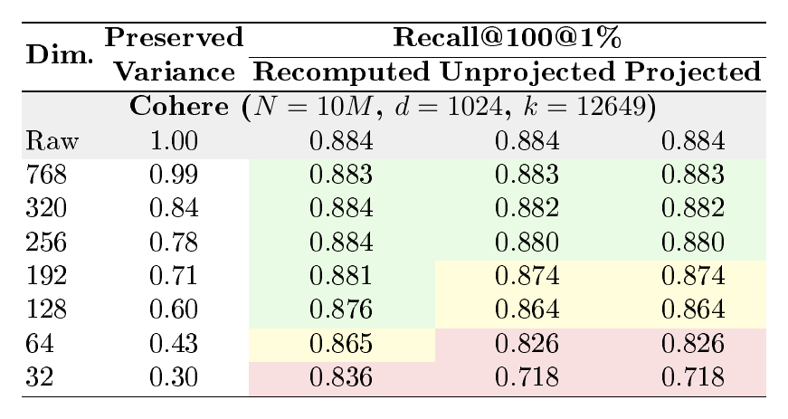
Dimensionality Reduction and Vector Search: Reducing the dimensionality of the raw vectors will affect index materialization, leading to three possible approaches: 1) recompute the full-dimensional centroids using cluster membership (requires access to raw vectors), 2) unproject centroids back to the original dimensionality (not possible when using Matryoshka vectors), and 3) utilize projected centroids for vector search in the reduced space [24]. The results shown in this section use approach #1. Table 6 shows a comparison of all strategies. Both unprojected and projected centroids yield lower clustering quality than recomputed full-dimensional centroids because energy from discarded dimensions is lost. However, the difference between the approaches is minimal at higher levels of preserved variance, allowing the pipeline to avoid accessing the raw vectors entirely after preprocessing. Previous studies have shown the feasibility of using projected vectors and centroids for vector search [24, 30], although these approaches still require storing the residuals of the PCA projection for re-ranking.

::: {caption="Table 6: Quality of the generated centroids when using three different strategies to materialize the centroids: recomputing centroids at full-d (best), unprojecting the centroids to the original dimensionality, and using the projected centroids."}

{width=60%}

:::

4.3 Mixing Techniques

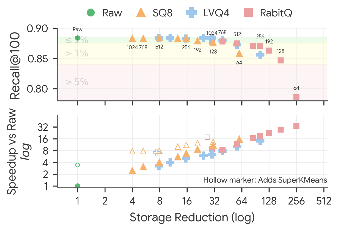
Figure 9 shows the result of combining techniques in our largest dataset (Cohere/1024). We present results for SQ8, LVQ4, and RabitQ, combined with PCA as dimensionality-reduction method. If maintaining quality equivalent to clustering raw vectors is essential, LVQ with 80% of preserved variance is the best choice. However, if quality can deviate by up to 1% from the optimal value, then RabitQ with 80% of PCA variance becomes the preferred option. For prioritizing speed while still aiming for near-optimal quality, RabitQ combined with SuperKMeans is the optimal choice. It is worth noting that using RabitQ with PCA and SuperKMeans can degrade performance due to the additional floating-point operations required to compute partial L2 distances for pruning, particularly for thinner vectors. In contrast, SQ8 consistently benefits from SuperKMeans because its distance calculations do not require any additional adjustments.

{width=60%}

4.4 Other Accelerators

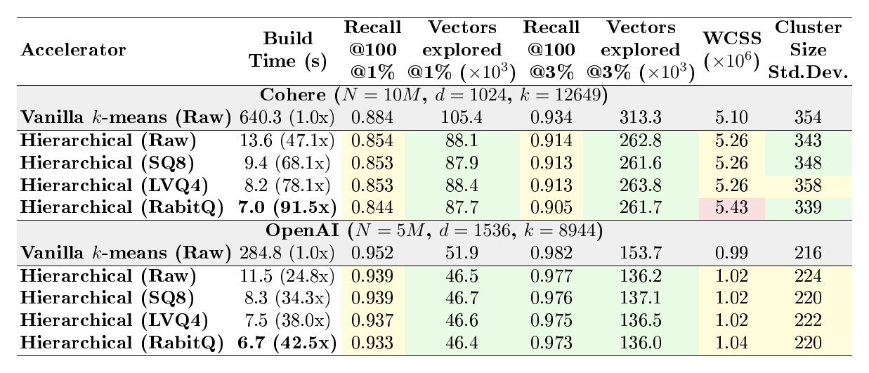
Hierarchical k-Means: Hierarchical $k$-means [92] has recently emerged as an alternative for clustering large collections of vector embeddings [23, 7, 64, 93, 16, 21, 11] because it reduces the complexity of vanilla $k$-means from $O(N * k * d)$ to $O(N * \sqrt{k} * d)$ by dividing the clustering process into two phases: MESO- and FINE-CLUSTERING. In the MESO-CLUSTERING phase, a coarser clustering is performed, creating only $\sqrt{k}$ clusters. In the subsequent FINE-CLUSTERING phase, $k$-means is applied within each meso-cluster, with the number of clusters set to $\sqrt{n_{i}}$, where $n_{i}$ is the number of points in the i-th meso-cluster. Finally, an optional refinement iteration of vanilla $k$-means can be performed to improve clustering quality further. Table 7 shows the quality of the resulting centroids for vector search tasks on our two largest datasets, Cohere and OpenAI, when using hierarchical $k$-means. The performance gains are remarkable, reaching up to 91x when hierarchical $k$-means is combined with RabitQ. Note that hierarchical $k$-means produces clusters with more uniform sizes in dense regions of the space, as indicated by the lower number of vectors explored. Nonetheless, this improved balance negatively affects recall and requires probing more clusters.

::: {caption="Table 7: Quality of the generated centroids for VSS using hierarchical k-means. Hierarchical k-means achieves remarkable speedups while producing more balanced clusters."}

:::

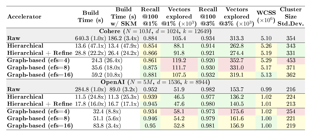
::: {caption="Table 8: Quality of the generated centroids for VSS tasks when using hierarchical k-means and graph-based assignments with HNSW."}

:::

Graph-based Assignments: Graph-based indexes for VSS have recently been used to determine assignments during clustering [94, 24]. This approach builds a graph-based vector index over the centroids (e.g., HNSW [53]). Consequently, determining assignments becomes a series of top-1 searches on the graph index. Both hierarchical $k$-means and graph-based assignments help clustering scale to larger datasets. Table 8 compares their performance on Cohere and OpenAI—our two largest datasets. For the graph-based assignment approach, we created an HNSW index using codewordef_construction = 128 and codewordM=16. We use a vanilla implementation of HNSW from the FAISS library [95]. Additionally, we incorporated an optimization that starts the graph traversal from the centroid assigned in the previous $k$-means iteration [24].

Both methods significantly accelerate clustering compared to vanilla $k$-means. However, graph-based assignments produce less balanced clusters, leading to more vectors explored during VSS. Additionally, the graph-based approach introduces the added complexity of tuning the codewordef_search parameter, which controls search quality. If this value is set too low, it improves speed but compromises clustering quality. Conversely, if set too high, it reduces speed improvements. Note that the graph construction over the centroids takes less than 0.1% of the total runtime.

Sampling: Sampling reduces clustering runtime proportionally to the fraction of vectors sampled from the data [11, 22]. Sampling around 20–30% of the data is sufficient to maintain clustering quality and balance [11]. Sampling can be used in conjunction with our proposed pipeline. However, note that the final assignment step and index materialization still need to use all vectors.

4.5 Scalability

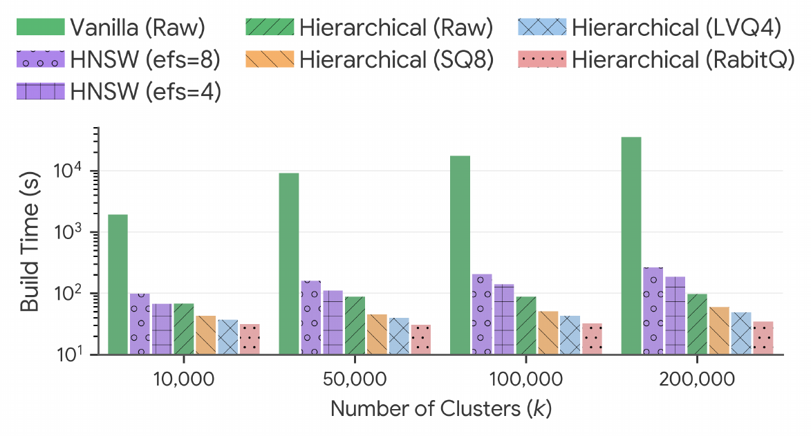
The optimal ratio of points per cluster varies depending on the application. Recent studies suggest that a lower points-per-cluster ratio (i.e., a higher $k$) is beneficial for vector search indexes [24]. Consequently, the scalability of our pipeline with respect to $k$ is critical. For this scalability experiment, we scale our Cohere dataset to 50M embeddings [82], totaling 200GB of data, and run our pipeline while progressively increasing the number of clusters to create ($k$). Additionally, we scale our machine to 512GB of RAM and 64 cores (codewordr8a.16xlarge in AWS). Figure 10 shows the results of this experiment. Hierarchical $k$-means with RabitQ vectors is the fastest approach: even when creating 200K clusters, centroid training remains under 1 minute. Notably, both hierarchical $k$-means and graph-based assignments scale sublinearly with respect to the number of clusters. This sublinear scalability is essential for indexing large vector collections, which would otherwise require several hours. The latter, combined with the clustering of quantized vectors, facilitates scalability in both storage requirements and runtime, all while maintaining index quality (as shown in Table 7).

{width=70%}

5. Discussion

Section Summary: Recent research on large-scale vector systems shows that clustering remains the standard way to organize data efficiently in cloud environments where every bit of computing time adds to the bill. The study finds that using full-precision vectors for this clustering step is unnecessary, and that applying the same approximation methods already used for search—such as quantization or dimensionality reduction—can speed up data ingestion instead. This unified approach lets systems reuse one simplified vector representation for both searching and indexing, opening the door to new techniques designed to handle both tasks at once.

Vector indexing through clustering remains the preferred method for large-scale cloud vector systems [7, 12, 3, 71], where every second of compute counts towards billing. The insights presented in this study show that using full-precision vectors for clustering is excessive: systems can improve the performance of data ingestion pipelines by first applying approximation techniques [24], wherein method selection can be guided by the algorithms used in the vector search pipeline. For instance, systems using LVQ for vector search [96] should apply the encoding before the clustering pipeline. The same applies to dimensionality reduction techniques, as recent studies propose combining them with quantization [30, 28, 29, 45, 24]. Ultimately, our design allows the same vector representations to be used for both vector search and clustering, enabling more streamlined indexing and ingestion in vector systems. The latter opens new research directions toward quantization techniques that can efficiently serve a dual purpose: efficient search and indexing.

6. Conclusions and Future Work

Section Summary: The researchers presented a new clustering method for organizing large sets of vector data, applying speed-up tricks such as data compression and dimension reduction before the actual grouping step. Tests showed these shortcuts cut storage needs by as much as 60 times and made the process much faster, while still producing results nearly as good as the full-precision approach. They also outlined plans to test the method on specialized computer hardware, graph-based data structures, and additional types of datasets to broaden its usefulness.

We have introduced a clustering pipeline for indexing vector embeddings in which approximation techniques commonly used for vector search are applied before clustering. Our experiments indicate that clustering is highly resilient to approximation techniques and show that even aggressive encodings (RabitQ), combined with dimensionality reduction (PCA) and dimension pruning (SuperKMeans), can reduce storage by up to 60x and substantially accelerate clustering, all while maintaining near-optimal clustering quality. Another striking feat of our study is the adaptation of quantization techniques for clustering pipelines and their integration with dimension pruning.

In future work, we aim to explore how the availability of specialized hardware units for specific data types (e.g., Intel's AMX) can lead to different trade-offs between speed and storage reduction. Additionally, replicating our study with graph-based indexes (e.g., HNSW, DiskANN) remains a future research opportunity attractive for systems that implement graph-based vector indexes. In the context of the graph-based assignment approach, exploring the performance of different graph indexes or developing novel indexes tailored for this purpose could yield significant benefits. Finally, an evaluation using multi-vector embeddings [97] and classic vector datasets that do not stem from AI embedding models (e.g., SIFT, GIST) would broaden the applicability of our pipeline.

References

Section Summary: The references section compiles a list of academic papers, technical reports, and online resources centered on vector indexing, quantization methods, and approximate nearest-neighbor search in large-scale data systems. The entries emphasize clustering techniques such as k-means, specialized libraries like Faiss, and practical implementations for cloud and on-device databases. Most sources are recent, spanning 2022 to 2026, with a few foundational works from earlier decades.

[1] Lloyd, Stuart (1982). Least squares quantization in PCM. IEEE transactions on information theory. 28(2). pp. 129–137.

[2] Mohoney et al. (2025). Quake: Adaptive Indexing for Vector Search. arXiv preprint arXiv:2506.03437.

[3] Papakonstantinou et al. (2024). ScaNN for AlloyDB. https://services.google.com/fh/files/misc/scann_for_alloydb_whitepaper.pdf.

[4] Jääsaari et al. (2024). Lorann: Low-rank matrix factorization for approximate nearest neighbor search. Advances in Neural Information Processing Systems. 37. pp. 102121–102153.

[5] Guo et al. (2020). Accelerating large-scale inference with anisotropic vector quantization. In International Conference on Machine Learning. pp. 3887–3896.

[6] Gao et al. (2024). Practical and Asymptotically Optimal Quantization of High-Dimensional Vectors in Euclidean Space for Approximate Nearest Neighbor Search. arXiv preprint arXiv:2409.09913.

[7] (2025). turbopuffer: Serverless Vector and Full‑Text Search on Object Storage. Accessed: 2025-12-24. https://turbopuffer.com/.

[8] Douze et al. (2024). The faiss library. arXiv preprint arXiv:2401.08281.

[9] Shi et al. (2026). GPU-Native Approximate Nearest Neighbor Search with IVF-RaBitQ: Fast Index Build and Search. arXiv preprint arXiv:2602.23999.

[10] Pound et al. (2025). MicroNN: An On-device Disk-resident Updatable Vector Database. In Companion of the 2025 International Conference on Management of Data. pp. 608–621.

[11] Kuffo et al. (2026). A Super Fast K-means for Indexing Vector Embeddings. arXiv preprint arXiv:2603.20009.

[12] Databricks (2026). Decoupled by Design: Billion-Scale Vector Search. https://www.databricks.com/blog/decoupled-design-billion-scale-vector-search.

[13] Ramani et al. (2025). Panorama: Fast-Track Nearest Neighbors. arXiv preprint arXiv:2510.00566.

[14] Santhanam et al. (2022). PLAID: an efficient engine for late interaction retrieval. In Proceedings of the 31st ACM International Conference on Information & Knowledge Management. pp. 1747–1756.

[15] Zhu et al. (2025). An Experimental Evaluation of Hybrid Querying on Vectors. Proceedings of the VLDB Endowment. 19(2). pp. 183–195.

[16] Xu et al. (2023). Spfresh: Incremental in-place update for billion-scale vector search. In Proceedings of the 29th Symposium on Operating Systems Principles. pp. 545–561.

[17] Mageirakos et al. (2025). Cracking Vector Search Indexes. arXiv preprint arXiv:2503.01823.

[18] Li et al. (2025). Cloud-Native Vector Search: A Comprehensive Performance Analysis. arXiv preprint arXiv:2511.14748.

[19] Kuffo, Leonardo and Boncz, Peter (2025). Bang for the Buck: Vector Search on Cloud CPUs. In Proceedings of the 21st International Workshop on Data Management on New Hardware. pp. 1–8.

[20] Matsui et al. (2017). Pqk-means: Billion-scale clustering for product-quantized codes. In Proceedings of the 25th ACM international conference on Multimedia. pp. 1725–1733.

[21] Martinico et al. (2026). Efficient Multivector Retrieval with Token-Aware Clustering and Hierarchical Indexing. In Proceedings of the 49th International ACM SIGIR Conference on Research and Development in Information Retrieval. pp. 3982–3987.

[22] Junyu Chen (2025). How We Made 100M Vector Indexing in 20 Minutes Possible on PostgreSQL. https://blog.vectorchord.ai/how-we-made-100m-vector-indexing-in-20-minutes-possible-on-postgresql.

[23] Thomas Veasey (2025). K-means for building vector indices. https://www.elastic.co/search-labs/blog/k-means-for-vector-indices.

[24] Wang et al. (2026). LindormVector: A Distributed Vector Engine on a Cloud-Native Multi-Model NoSQL Database. In Companion of the International Conference on Management of Data. pp. 451–463.

[25] Boutsidis et al. (2010). Random projections for $ k $-means clustering. Advances in neural information processing systems. 23.

[26] Johnson et al. (1984). Extensions of Lipschitz mappings into a Hilbert space. Contemporary mathematics. 26(189-206). pp. 1.

[27] Abdi, Hervé and Williams, Lynne J (2010). Principal component analysis. Wiley interdisciplinary reviews: computational statistics. 2(4). pp. 433–459.

[28] Tepper et al. (2023). LeanVec: Searching vectors faster by making them fit. arXiv preprint arXiv:2312.16335.

[29] Tepper et al. (2024). GleanVec: Accelerating vector search with minimalist nonlinear dimensionality reduction. arXiv preprint arXiv:2410.22347.

[30] Yang et al. (2024). Quantization Meets Projection: A Happy Marriage for Approximate k-Nearest Neighbor Search. arXiv preprint arXiv:2411.06158.

[31] Kusupati et al. (2022). Matryoshka representation learning. Advances in Neural Information Processing Systems. 35. pp. 30233–30249.

[32] Aguerrebere et al. (2023). Similarity search in the blink of an eye with compressed indices. arXiv preprint arXiv:2304.04759.

[33] Gao, Jianyang and Long, Cheng (2024). RaBitQ: Quantizing High-Dimensional Vectors with a Theoretical Error Bound for Approximate Nearest Neighbor Search. Proceedings of the ACM on Management of Data. 2(3). pp. 1–27.

[34] Dwango Media Village (2017). pqkmeans: Product Quantization k-means clustering. https://github.com/DwangoMediaVillage/pqkmeans.

[35] Jegou et al. (2010). Product quantization for nearest neighbor search. IEEE transactions on pattern analysis and machine intelligence. 33(1). pp. 117–128.

[36] Kuffo et al. (2025). PDX: A Data Layout for Vector Similarity Search. Proceedings of the ACM on Management of Data. 3(3). pp. 1–26.

[37] Zheng et al. (2026). Distance Comparison Operations Are Not Silver Bullets in Vector Similarity Search: A Benchmark Study on Their Merits and Limits. arXiv preprint arXiv:2604.02801.

[38] Wang et al. (2026). Distance Comparison Operation Optimization in ANNS: A Survey and Experimental Evaluation.. In EDBT. pp. 578–591.

[39] Gao, Jianyang and Long, Cheng (2023). High-dimensional approximate nearest neighbor search: with reliable and efficient distance comparison operations. Proceedings of the ACM on Management of Data. 1(2). pp. 1–27.

[40] Deng et al. (2024). Efficient data-aware distance comparison operations for high-dimensional approximate nearest neighbor search. arXiv preprint arXiv:2411.17229.

[41] Pace et al. (2025). Lance: Efficient Random Access in Columnar Storage through Adaptive Structural Encodings. arXiv preprint arXiv:2504.15247.

[42] Wang et al. (2021). Milvus: A purpose-built vector data management system. In Proceedings of the 2021 International Conference on Management of Data. pp. 2614–2627.

[43] Zandieh et al. (2025). Turboquant: Online vector quantization with near-optimal distortion rate. arXiv preprint arXiv:2504.19874.

[44] Wei et al. (2025). Subspace Collision: An Efficient and Accurate Framework for High-dimensional Approximate Nearest Neighbor Search. Proceedings of the ACM on Management of Data. 3(1). pp. 1–29.

[45] Li et al. (2025). SAQ: Pushing the Limits of Vector Quantization through Code Adjustment and Dimension Segmentation. Proceedings of the ACM on Management of Data. 3(6). pp. 1–25.

[46] Gou et al. (2025). SymphonyQG: towards symphonious integration of quantization and graph for approximate nearest neighbor search. Proceedings of the ACM on Management of Data. 3(1). pp. 1–26.

[47] Sun et al. (2023). SOAR: improved indexing for approximate nearest neighbor search. Advances in Neural Information Processing Systems. 36. pp. 3189–3204.

[48] Wei et al. (2026). PDET-LSH: Scalable In-Memory Indexing for High-Dimensional Approximate Nearest Neighbor Search with Quality Guarantees. IEEE Transactions on Knowledge and Data Engineering.

[49] Chen et al. (2021). Spann: Highly-efficient billion-scale approximate nearest neighborhood search. Advances in Neural Information Processing Systems. 34. pp. 5199–5212.

[50] Azizi et al. (2023). Elpis: Graph-based similarity search for scalable data science. Proceedings of the VLDB Endowment. 16(6). pp. 1548–1559.

[51] Tatsuno et al. (2024). AiSAQ: All-in-Storage ANNS with Product Quantization for DRAM-free Information Retrieval. arXiv preprint arXiv:2404.06004.

[52] Jayaram Subramanya et al. (2019). Diskann: Fast accurate billion-point nearest neighbor search on a single node. Advances in Neural Information Processing Systems. 32.

[53] Malkov, Yu A and Yashunin, Dmitry A (2018). Efficient and robust approximate nearest neighbor search using hierarchical navigable small world graphs. IEEE transactions on pattern analysis and machine intelligence. 42(4). pp. 824–836.

[54] Manohar et al. (2024). Parlayann: Scalable and deterministic parallel graph-based approximate nearest neighbor search algorithms. In Proceedings of the 29th ACM SIGPLAN Annual Symposium on Principles and Practice of Parallel Programming. pp. 270–285.

[55] Xu et al. (2025). In-place updates of a graph index for streaming approximate nearest neighbor search. arXiv preprint arXiv:2502.13826.

[56] Patel et al. (2024). Acorn: Performant and predicate-agnostic search over vector embeddings and structured data. Proceedings of the ACM on Management of Data. 2(3). pp. 1–27.

[57] Gollapudi et al. (2023). Filtered-diskann: Graph algorithms for approximate nearest neighbor search with filters. In Proceedings of the ACM Web Conference 2023. pp. 3406–3416.

[58] Lu et al. (2026). An in-depth study of filter-agnostic vector search on a postgresql database system:[experiments & analysis]. Proceedings of the ACM on Management of Data. 4(3 (SIGMOD). pp. 1–26.

[59] Tekin, Selim Furkan and Bordawekar, Rajesh (2025). B+ ANN: A Fast Billion-Scale Disk-based Nearest-Neighbor Index. arXiv preprint arXiv:2511.15557.

[60] Mortensen et al. (2023). Marigold: efficient k-means clustering in high dimensions. Proceedings of the VLDB Endowment. 16(7). pp. 1740–1748.

[61] Arthur, David and Vassilvitskii, Sergei (2006). k-means++: The advantages of careful seeding.

[62] Zhakubayev, Alibek and Hamerly, Greg (2024). Using Annealing to Accelerate Triangle Inequality k-means. In 2024 IEEE 11th International Conference on Data Science and Advanced Analytics (DSAA). pp. 1–9.

[63] Xie et al. (2025). Fast approximate similarity join in vector databases. Proceedings of the ACM on Management of Data. 3(3). pp. 1–26.

[64] RAPIDS AI (2025). rapidsai/cuVS: GPU-Accelerated Vector Search and Clustering Library. https://github.com/rapidsai/cuvs. Accessed: 2026-01-21.

[65] Gates et al. (2026). Vortex. https://github.com/vortex-data/vortex.

[66] Forgy, Edward W (1965). Cluster analysis of multivariate data: efficiency versus interpretability of classifications. biometrics. 21. pp. 768–769.

[67] RAPIDS AI (2026). K-Means — cuVS C++ API Documentation (stable 26.04).

[68] Zhakubayev, Alibek and Hamerly, Greg (2022). Clustering faster and better with projected data. In Proceedings of the 6th International Conference on Information System and Data Mining. pp. 1–6.

[69] Pan et al. (2023). Survey of vector database management systems. arXiv preprint arXiv:2310.14021.

[70] Aguerrebere et al. (2024). Locally-Adaptive Quantization for Streaming Vector Search. arXiv preprint arXiv:2402.02044.

[71] Xu et al. (2025). Harmony: A scalable distributed vector database for high-throughput approximate nearest neighbor search. Proceedings of the ACM on Management of Data. 3(4). pp. 1–28.

[72] Vardanian, Ash. NumKong: 2000 Mixed Precision Kernels For All. https://github.com/ashvardanian/NumKong.

[73] Deng et al. (2025). Demystifying ARM SME to Optimize General Matrix Multiplications. arXiv preprint arXiv:2512.21473.

[74] Unity Technologies (n.d.). Unity.Burst.Intrinsics.Arm.Neon.vdotq_s32 Method. Arm NEON dot-product intrinsic (SDOT equivalent); Accessed: 2026-05-06. https://docs.unity3d.com/Packages/[email protected]/api/Unity.Burst.Intrinsics.Arm.Neon.vdotq_s32.html.

[75] Félix Cloutier (n.d.). VPDPBUSD — Multiply and Add Unsigned and Signed Bytes. x86 instruction reference; Accessed: 2026-05-06. https://www.felixcloutier.com/x86/vpdpbusd.

[76] Intel Corporation (2024). What Is Intel® Advanced Matrix Extensions (Intel® AMX)?. Accessed: 2026-05-06. https://www.intel.com/content/www/us/en/products/docs/accelerator-engines/what-is-intel-amx.html.

[77] Kim et al. (2024). Exploiting intel advanced matrix extensions (AMX) for large language model inference. IEEE Computer Architecture Letters. 23(1). pp. 117–120.

[78] Kuffo et al. (2026). Semantic Recall for Vector Search. In Proceedings of the 49th International ACM SIGIR Conference on Research and Development in Information Retrieval. pp. 3907–3912.

[79] André et al. (2016). Cache locality is not enough: High-performance nearest neighbor search with product quantization fast scan. In 42nd International Conference on Very Large Data Bases. pp. 12.

[80] Google (2026). ruy: The ruy Matrix Multiplication Library. https://github.com/google/ruy. GitHub repository, accessed 2026-05-31.

[81] Félix Cloutier (n.d.). PSHUFB — Packed Shuffle Bytes. x86 instruction reference (SSSE3/AVX/AVX-512); Accessed: 2026-05-06. https://www.felixcloutier.com/x86/pshufb.

[82] Cohere Labs (2024). TREC-RAG 2024 Corpus (MSMARCO 2.1) - Encoded with Cohere Embed English v3). https://huggingface.co/datasets/CohereLabs/msmarco-v2.1-embed-english-v3.

[83] Qdrant (2024). DBpedia Entities with OpenAI text-embedding-3-large (1536-dim, 1M vectors). https://huggingface.co/datasets/Qdrant/dbpedia-entities-openai3-text-embedding-3-large-1536-1M.

[84] Qdrant (2023). arXiv Titles Instructor XL Embeddings (768-dim, 2.25M vectors). https://huggingface.co/datasets/Qdrant/arxiv-titles-instructorxl-embeddings.

[85] Daria Kryvosheieva et al. (2025). Efficient Code Embeddings from Code Generation Models. https://arxiv.org/abs/2508.21290. arXiv:2508.21290.

[86] Jääsaari et al. (2025). VIBE: Vector Index Benchmark for Embeddings. arXiv preprint arXiv:2505.17810.

[87] Sean Lee et al. (2024). Open Source Strikes Bread – New Fluffy Embeddings Model. https://www.mixedbread.ai/blog/mxbai-embed-large-v1.

[88] Deng et al. (2009). Imagenet: A large-scale hierarchical image database. In 2009 IEEE conference on computer vision and pattern recognition. pp. 248–255.

[89] CWI Database Architectures Group (2026). SuperKMeans. https://github.com/cwida/SuperKMeans.

[90] OpenBLAS Contributors (2026). OpenBLAS: An optimized BLAS library. https://github.com/OpenMathLib/OpenBLAS.

[91] Masliah et al. (2016). High-performance matrix-matrix multiplications of very small matrices. In European Conference on Parallel Processing. pp. 659–671.

[92] Steinbach et al. (2000). A comparison of document clustering techniques.

[93] Jin et al. (2026). Curator: Efficient Vector Search with Low-Selectivity Filters. Proceedings of the ACM on Management of Data. 4(1 (SIGMOD). pp. 1–27.

[94] Spalding-Jamieson et al. (2025). Scalable k-Means Clustering for Large k via Seeded Approximate Nearest-Neighbor Search. arXiv preprint arXiv:2502.06163.

[95] Meta Research (2024). Faiss: A library for efficient similarity search and clustering of dense vectors.. https://github.com/facebookresearch/faiss.

[96] Intel (2025). Scalable Vector Search. https://github.com/intel/ScalableVectorSearch. GitHub repository, accessed 2026-05-15.

[97] Khattab, Omar and Zaharia, Matei (2020). Colbert: Efficient and effective passage search via contextualized late interaction over bert. In Proceedings of the 43rd International ACM SIGIR conference on research and development in Information Retrieval. pp. 39–48.