Accelerated Coordinate Encoding: Learning to Relocalize in Minutes Using RGB and Poses

Eric BrachmannTommaso CavallariVictor Adrian Prisacariu

article2023CVPR174 citations

Presents Accelerated Coordinate Encoding, an approach that trains accurate visual relocalization models in under five minutes from posed RGB images alone, speeding up scene coordinate mapping by up to 300 times compared to existing methods.

Listen

Visual relocalization is essential for real-time applications such as augmented reality, mobile robotics, and navigation, where a system must quickly determine a camera's precise position and orientation within an environment. While learning-based methods achieve high accuracy and generate compact, privacy-preserving scene representations, they traditionally require hours or days of retraining for every single new scene. This extensive mapping delay creates a major operational bottleneck and incurs high computational and financial costs, severely limiting the real-world viability of learning-based relocalizers.

The article introduces Accelerated Coordinate Encoding (ACE), a visual relocalization pipeline designed to train scene coordinate regression networks in under five minutes while matching or exceeding the accuracy of state-of-the-art methods.

To achieve this, the article separates the relocalization architecture into a fixed, scene-agnostic convolutional feature extractor and a small, scene-specific multi-layer perceptron. In the first minute of mapping, the feature extractor processes standard RGB images and their known camera positions into an 8-million-feature training buffer. Over the next four minutes, the regression network samples randomized patches across thousands of distinct camera views in parallel batches. This process eliminates correlated gradient updates, allowing the system to use high learning rates safely. The framework also replaces slow end-to-end optimization with an adaptive curriculum over a reprojection loss, using a smoothly tightening error boundary to focus model capacity on reliable geometry without needing dedicated depth sensors or 3D meshes.

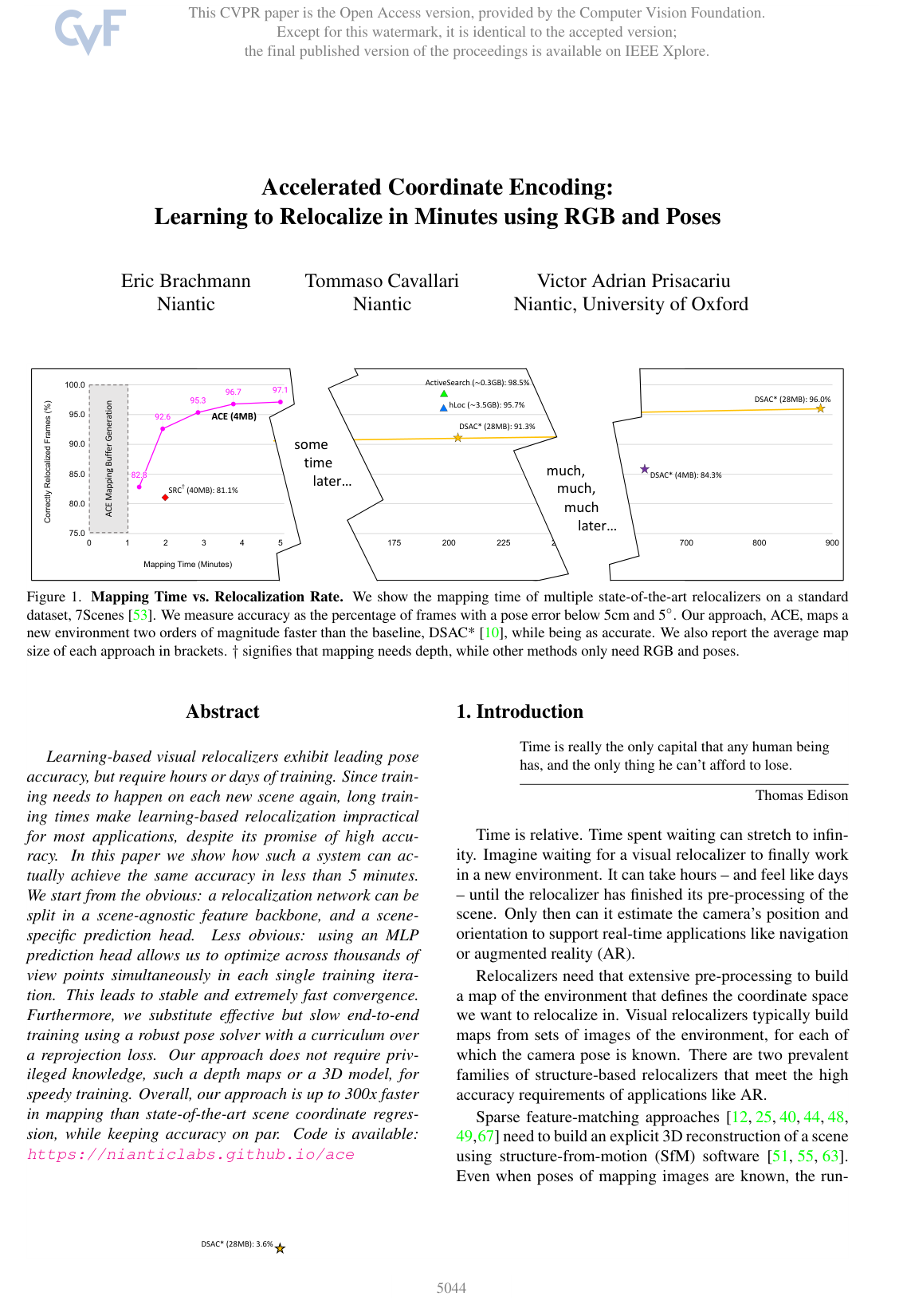
Evaluations across indoor and outdoor benchmarks demonstrate that ACE maps environments up to 300 times faster than the leading baseline, DSAC*. On indoor benchmarks, ACE mapped scenes in five minutes and achieved a 97.1% success rate on 7Scenes and 99.9% on 12Scenes, matching the accuracy of systems that took 11 to 15 hours to train. On outdoor phone scans from the Wayspots dataset, ACE attained a 52.2% average relocalization rate, outperforming the full baseline's 50.7%. Furthermore, ACE compresses complete scene environments into 4MB map files—reducing storage needs by up to seven times compared to prior neural relocalizers and hundreds of times compared to traditional point-cloud methods. Additionally, ACE proved resilient to budget compute hardware, incurring only a 10% training slowdown on low-cost GPUs where traditional baselines doubled their training times to 28 hours.

These results demonstrate that fast, accurate, and low-cost visual mapping can be achieved on standard consumer devices without requiring specialized depth cameras or costly 3D reconstruction pipelines. By lowering training compute time from 15 hours to under five minutes on budget hardware, the method reduces infrastructure costs, lowers energy consumption, and enables on-demand mapping for dynamic user environments.

Organizations developing spatial computing, augmented reality, or robotics platforms should consider adopting decoupled architectures and patch-decorrelation training workflows to eliminate scene pre-processing bottlenecks. When deploying to expansive outdoor environments, teams can explore multi-model ensembles, as demonstrated by the quad-model variant in the article, to balance map footprint against geometric coverage. Further engineering improvements, such as running buffer generation and network training on parallel execution threads, should be prioritized to reduce mapping latency even further.

Decision-makers should note that ACE relies on known initial mapping camera poses, typically supplied by standard visual odometry or structure-from-motion tools, and performance can still degrade in highly repetitive or untextured outdoor scenes. Nonetheless, the empirical evidence provides high confidence that ACE establishes a practical, highly scalable standard for learning-based visual relocalization.

arXiv: 2305.14059

No sufficiently relevant recommendations were found.
Cover for Accelerated Coordinate Encoding: Learning to Relocalize in Minutes Using RGB and Poses

Abstract

Learning-based visual relocalizers exhibit leading pose accuracy, but require hours or days of training. Since training needs to happen on each new scene again, long training times make learning-based relocalization impractical for most applications, despite its promise of high accuracy. In this paper we show how such a system can actually achieve the same accuracy in less than 5 minutes. We start from the obvious: a relocalization network can be split in a scene-agnostic feature backbone, and a scene-specific prediction head. Less obvious: using an MLP prediction head allows us to optimize across thousands of view points simultaneously in each single training iteration. This leads to stable and extremely fast convergence. Furthermore, we substitute effective but slow end-to-end training using a robust pose solver with a curriculum over a reprojection loss. Our approach does not require privileged knowledge, such as depth maps or a 3D model, for speedy training. Overall, our approach is up to 300x faster in mapping than state-of-the-art scene coordinate regression, while keeping accuracy on par. Code is available: https://nianticlabs.github.io/ace

Table of Contents

  • 1. Introduction
  • 2. Related Work
  • 3. Method
  • 3.1. Efficient Training by Gradient Decorrelation
  • 3.2. Curriculum Training
  • 3.3. Backbone Training
  • 3.4. Further Improvements
  • 4. Experiments
  • 4.1. Indoor Relocalization
  • 4.2. Outdoor Relocalization
  • 4.3. Analysis
  • 5. Conclusion and Future Work
  • References

Knowls

  1. Knowl 1 — Accelerated Coordinate Encoding Architecture and Network Split

    model/method

    Accelerated Coordinate Encoding (ACE) decomposes scene coordinate regression into a two-part neural architecture: a scene-agnostic feature backbone fBf_\text{B} and a scene-specific prediction head fHf_\text{H}. Given an RGB image II and a 2D pixel coordinate xi\mathbf{x}_i, an image patch pi=P(xi,I)∈RCI×HP×WP\mathbf{p}_i = \mathcal{P}(\mathbf{x}_i, I) \in \mathbb{R}^{C_\text{I} \times H_\text{P} \times W_\text{P}} (typically grayscale with CI=1C_\text{I}=1 and spatial dimensions HP=WP=81pxH_\text{P} = W_\text{P} = 81\text{px}) is mapped to a predicted 3D scene coordinate yi∈R3\mathbf{y}_i \in \mathbb{R}^3 via:

    yi=f(pi;w)=fH(fB(pi;wB);wH)\mathbf{y}_i = f(\mathbf{p}_i; \mathbf{w}) = f_\text{H}(f_\text{B}(\mathbf{p}_i; \mathbf{w}_\text{B}); \mathbf{w}_\text{H})

    where w={wB,wH}\mathbf{w} = \{\mathbf{w}_\text{B}, \mathbf{w}_\text{H}\} are network parameters.

    The backbone fB:RCI×HP×WP→RCff_\text{B}: \mathbb{R}^{C_\text{I} \times H_\text{P} \times W_\text{P}} \to \mathbb{R}^{C_f} is a fully convolutional neural network that extracts a dense feature vector fi∈RCf\mathbf{f}_i \in \mathbb{R}^{C_f}. The scene-specific head fH:RCf→R3f_\text{H}: \mathbb{R}^{C_f} \to \mathbb{R}^3 is a multi-layer perceptron (MLP) implemented using shared-weight 1×11 \times 1 convolutions. Because fHf_\text{H} operates on point-wise feature vectors without requiring spatial context across neighboring pixels, feature representations extracted from across an entire mapping image collection can be pooled, shuffled, and sampled independently during scene-specific training.

  2. Knowl 2 — ACE Two-Stage Mapping Algorithm with Gradient Decorrelation

    algorithm

    ACE maps a new scene from a set of posed RGB mapping images IM={(Im,hm∗,Km)}m=1M\mathcal{I}_\text{M} = \{(I_m, \mathbf{h}_m^*, \mathbf{K}_m)\}_{m=1}^M using a two-stage training procedure. In Stage 1 (Buffer Generation, taking approximately 1 minute), the pre-trained, frozen backbone fBf_\text{B} extracts high-dimensional feature descriptors across all mapping frames to populate a fixed-size feature buffer containing 8×1068 \times 10^6 entries. In Stage 2 (MLP Training Loop, taking approximately 4 minutes), the scene-specific MLP fHf_\text{H} is trained for 16 epochs using large minibatches drawn uniformly from the shuffled buffer.

    Input: Mapping dataset IM={(Im,hm∗,Km)}m=1M\mathcal{I}_\text{M} = \{(I_m, \mathbf{h}_m^*, \mathbf{K}_m)\}_{m=1}^M, pre-trained backbone fBf_\text{B}, batch size B=5120B=5120, total epochs E=16E=16, learning rate schedule OneCycleLR(5×10−4,5×10−3)\text{OneCycleLR}(5\times 10^{-4}, 5\times 10^{-3})
    Output: Trained scene-specific MLP head weights wH\mathbf{w}_\text{H}
    Initialize empty buffer B←∅\mathcal{B} \leftarrow \emptyset
    for each (Im,hm∗,Km)∈IM(I_m, \mathbf{h}_m^*, \mathbf{K}_m) \in \mathcal{I}_\text{M} do
        Extract dense feature map Fm=fB(Im)\mathbf{F}_m = f_\text{B}(I_m)
        for sampled pixel locations xi\mathbf{x}_i in image mm do
            Extract feature vector fi=Fm[xi]\mathbf{f}_i = \mathbf{F}_m[\mathbf{x}_i]
            B←B∪{(fi,xi,hm∗,Km)}\mathcal{B} \leftarrow \mathcal{B} \cup \{(\mathbf{f}_i, \mathbf{x}_i, \mathbf{h}_m^*, \mathbf{K}_m)\}
        end for
    end for
    Initialize MLP weights wH\mathbf{w}_\text{H} in float16 precision
    for epoch e=1e = 1 to EE do
        Shuffle buffer B\mathcal{B}
        for each batch S⊂B\mathcal{S} \subset \mathcal{B} of size BB do
            Compute relative progress t∈(0,1)t \in (0, 1)
            Update curriculum threshold τ(t)=1−t2⋅τmax+τmin\tau(t) = \sqrt{1 - t^2} \cdot \tau_\text{max} + \tau_\text{min}
            Compute loss L=1∣S∣∑(fi,xi,hi∗,Ki)∈Sℓπ(xi,fH(fi;wH),hi∗,Ki,τ(t))L = \frac{1}{|\mathcal{S}|} \sum_{(\mathbf{f}_i, \mathbf{x}_i, \mathbf{h}_i^*, \mathbf{K}_i) \in \mathcal{S}} \ell_\pi(\mathbf{x}_i, f_\text{H}(\mathbf{f}_i; \mathbf{w}_\text{H}), \mathbf{h}_i^*, \mathbf{K}_i, \tau(t))
            Update wH\mathbf{w}_\text{H} via AdamW optimizer with current scheduled learning rate
        end for
    end for
    return wH\mathbf{w}_\text{H}

    Sampling patches across thousands of distinct mapping views within every single minibatch decorrelates training gradients, providing gradient stability that allows aggressive learning rates.

  3. Knowl 3 — Curriculum Reprojection Loss with Dynamic Tanh Clamping

    equation

    To eliminate the need for computationally expensive end-to-end differentiable RANSAC pose optimization during mapping, ACE optimizes a pixel-level reprojection loss governed by a dynamic inlier-clamping curriculum:

    ℓπ(xi,yi,hi∗)={e^π(xi,yi,hi∗)if yi∈V∥yi−yˉi∥0otherwise\ell_\pi(\mathbf{x}_i, \mathbf{y}_i, \mathbf{h}_i^*) = \begin{cases} \hat{e}_\pi(\mathbf{x}_i, \mathbf{y}_i, \mathbf{h}_i^*) & \text{if } \mathbf{y}_i \in \mathcal{V} \\ \|\mathbf{y}_i - \bar{\mathbf{y}}_i\|_0 & \text{otherwise} \end{cases}

    where xi∈R2\mathbf{x}_i \in \mathbb{R}^2 is the 2D image pixel location, yi∈R3\mathbf{y}_i \in \mathbb{R}^3 is the predicted 3D scene coordinate, and hi∗\mathbf{h}_i^* is the ground-truth rigid camera pose. The valid coordinate set V\mathcal{V} contains predictions located between 0.10m0.10\text{m} and 1000m1000\text{m} in front of the camera plane with reprojection error eπ<1000pxe_\pi < 1000\text{px}. For invalid predictions yi∉V\mathbf{y}_i \notin \mathcal{V}, the loss penalizes the distance to a fallback coordinate yˉi\bar{\mathbf{y}}_i computed from hi∗\mathbf{h}_i^* at an assumed depth of 10m10\text{m}.

    The robust reprojection error e^π\hat{e}_\pi is clamped using a hyperbolic tangent scaled by a time-varying threshold τ(t)\tau(t):

    e^π(xi,yi,hi∗)=τ(t)tanh⁡(eπ(xi,yi,hi∗)τ(t))\hat{e}_\pi(\mathbf{x}_i, \mathbf{y}_i, \mathbf{h}_i^*) = \tau(t) \tanh\left(\frac{e_\pi(\mathbf{x}_i, \mathbf{y}_i, \mathbf{h}_i^*)}{\tau(t)}\right)

    τ(t)=w(t)τmax+τmin,with w(t)=1−t2\tau(t) = w(t) \tau_\text{max} + \tau_\text{min}, \quad \text{with } w(t) = \sqrt{1 - t^2}

    where t∈(0,1)t \in (0, 1) represents the fraction of total training completed, τmax=50px\tau_\text{max} = 50\text{px}, and τmin=1px\tau_\text{min} = 1\text{px}. The circular schedule keeps τ(t)\tau(t) loose early in training to guide coarse scene geometry before tightening towards τmin\tau_\text{min} at the end of training to refine high-precision structures.

  4. Knowl 4 — Homogeneous Coordinate Overparameterization with Softplus Clipping

    model/method

    In ACE, the scene-specific MLP head outputs an overparameterized 4D homogeneous coordinate representation y′=(x,y,z,w)⊤∈R4\mathbf{y}' = (x, y, z, w)^\top \in \mathbb{R}^4 rather than directly regressing 3D Euclidean coordinates (x,y,z)⊤(x, y, z)^\top.

    To ensure numerical stability and prevent sign ambiguity, the scalar scale parameter ww is constrained to be strictly positive via a softplus operation:

    wclipped=softplus(w)=ln⁡(1+ew)w_\text{clipped} = \text{softplus}(w) = \ln(1 + e^w)

    The Euclidean 3D scene coordinate y∈R3\mathbf{y} \in \mathbb{R}^3 supplied to the reprojection loss and subsequent PnP solver is then obtained by perspective division:

    y=(xwclipped,ywclipped,zwclipped)⊤\mathbf{y} = \left( \frac{x}{w_\text{clipped}}, \frac{y}{w_\text{clipped}}, \frac{z}{w_\text{clipped}} \right)^\top

  5. Knowl 5 — Multi-Head Bottleneck Pre-Training for Scene-Agnostic Feature Backbone

    model/method

    The scene-agnostic feature backbone fBf_\text{B} in ACE is trained to produce dense descriptors tailored for scene coordinate regression across arbitrary indoor and outdoor environments. Unlike descriptors engineered for sparse keypoint matching, the backbone must generate distinctive embeddings at every valid image coordinate.

    The backbone is pre-trained by connecting fBf_\text{B} to N=100N = 100 parallel scene-specific MLP regression heads, each corresponding to an independent training scene from the ScanNet dataset. The full multi-head network is trained jointly for one week using the curriculum reprojection loss. This multi-task bottleneck architecture prevents individual scene heads from overfitting while forcing fBf_\text{B} to encode universal geometric features. The resulting backbone weights require 11MB11\text{MB} of storage and remain completely frozen when mapping new scenes.

  6. Knowl 6 — Indoor Visual Relocalization Performance on 7Scenes and 12Scenes

    data/table

    ACE was evaluated against feature matching (FM) and scene coordinate regression (SCR) methods on the 7Scenes and 12Scenes benchmarks. Accuracy is reported as the percentage of test query frames estimated within 5cm5\text{cm} translation error and 5∘5^\circ rotation error under both SfM ground-truth poses and Depth-SLAM (D-SLAM) ground-truth poses.

    Method Depth Req. Map Time Map Size 7Scenes (SfM) 7Scenes (D-SLAM) 12Scenes (SfM)
    AS (SIFT) No ∼\sim1.5h ∼\sim200MB 98.5% 68.7% 99.8%
    D.VLAD+R2D2 No ∼\sim1.5h ∼\sim1GB 95.7% 77.6% 99.9%
    hLoc (SP+SG) No ∼\sim1.5h ∼\sim2GB 95.7% 76.8% 100%
    pixLoc No ∼\sim1.5h ∼\sim1GB N/A 75.7% N/A
    DSAC* (Full, w/ depth) Yes 15h 28MB 98.2% 84.0% 99.8%
    DSAC* (Tiny, w/ depth) Yes 11h 4MB 85.6% 70.0% 84.4%
    SANet Yes ∼\sim2.3 min ∼\sim550MB N/A 68.2% N/A
    SRC Yes 2 min 40MB 81.1% 55.2% N/A
    DSAC* (Full) No 15h 28MB 96.0% 81.1% 99.6%
    DSAC* (Tiny) No 11h 4MB 84.3% 69.1% 81.9%
    ACE (ours) No 5 min 4MB 97.1% 80.8% 99.9%

    ACE is the only method that achieves top-tier relocalization accuracy (97.1%97.1\% on 7Scenes SfM and 99.9%99.9\% on 12Scenes SfM) in under 10 minutes of mapping time, using under 10MB10\text{MB} of storage (4MB4\text{MB} per scene), while requiring strictly RGB images and poses without depth or 3D meshes.

  7. Knowl 7 — Outdoor Relocalization on Cambridge Landmarks and Poker Quad-Ensemble

    data/table

    ACE and an ensemble configuration denoted Poker were evaluated on the outdoor Cambridge Landmarks dataset. Results report median position error (in cm) and orientation error (in degrees) across five scenes. Poker partitions the mapping frames into four separate ACE sub-models (mapping time 20 min, total map size 16MB) and selects the pose hypothesis with the highest RANSAC inlier count during query time.

    Method Mapping Time Size Court King's Hospital Shop St. Mary's Average
    AS (SIFT) No ∼\sim35m ∼\sim200MB 24 / 0.1∘^\circ 13 / 0.2∘^\circ 20 / 0.4∘^\circ 4 / 0.2∘^\circ 8 / 0.3∘^\circ 14 / 0.2∘^\circ
    hLoc (SP+SG) No ∼\sim35m ∼\sim800MB 16 / 0.1∘^\circ 12 / 0.2∘^\circ 15 / 0.3∘^\circ 4 / 0.2∘^\circ 7 / 0.2∘^\circ 11 / 0.2∘^\circ
    PoseNet17 No 4–24h 50MB 683 / 3.5∘^\circ 88 / 1.0∘^\circ 320 / 3.3∘^\circ 88 / 3.8∘^\circ 157 / 3.3∘^\circ 267 / 3.0∘^\circ
    DSAC* (Full) No 15h 28MB 34 / 0.2∘^\circ 18 / 0.3∘^\circ 21 / 0.4∘^\circ 5 / 0.3∘^\circ 15 / 0.6∘^\circ 19 / 0.4∘^\circ
    DSAC* (Tiny) No 11h 4MB 98 / 0.5∘^\circ 27 / 0.4∘^\circ 33 / 0.6∘^\circ 11 / 0.5∘^\circ 56 / 1.8∘^\circ 45 / 0.8∘^\circ
    ACE (single) No 5m 4MB 43 / 0.2∘^\circ 28 / 0.4∘^\circ 31 / 0.6∘^\circ 5 / 0.3∘^\circ 18 / 0.6∘^\circ 25 / 0.4∘^\circ
    Poker (Quad ACE) No 20m 16MB 28 / 0.1∘^\circ 18 / 0.3∘^\circ 25 / 0.5∘^\circ 5 / 0.3∘^\circ 9 / 0.3∘^\circ 17 / 0.3∘^\circ

    A single 4MB ACE model maps an outdoor scene in 5 minutes with a median error of 25cm/0.4∘25\text{cm} / 0.4^\circ (outperforming DSAC* Tiny at 45cm/0.8∘45\text{cm} / 0.8^\circ), while the Poker ensemble achieves 17cm/0.3∘17\text{cm} / 0.3^\circ, outperforming the 15-hour DSAC* Full baseline (19cm/0.4∘19\text{cm} / 0.4^\circ).

  8. Knowl 8 — RGB-Only Visual Odometry Relocalization on the Wayspots Benchmark

    empirical result

    The Wayspots benchmark tests visual relocalization in practical mobile settings where mapping data consists of raw RGB phone video registered via visual odometry (without depth sensors or SfM 3D point clouds). On 10 outdoor scenes from the MapFree corpus evaluated under a 10cm,5∘10\text{cm}, 5^\circ threshold:

    1. ACE achieved an average accuracy of 52.2%52.2\% across all scenes with a 5-minute training time per scene.
    2. DSAC* Full achieved an average accuracy of 50.7%50.7\% after 15 hours of training per scene.
    3. DSAC* Tiny (4MB model) achieved an average accuracy of 43.6%43.6\% after 11 hours of training per scene.
    4. When DSAC* training was prematurely terminated after 5 minutes, its relocalization accuracy dropped to single-digit percentages.
  9. Knowl 9 — ACE Mapping Efficiency Across GPU Compute Tiers

    data/table

    Training speed and mapping turnaround times were evaluated across a high-end compute GPU (NVIDIA Tesla V100) and an entry-level budget GPU (NVIDIA Tesla T4):

    GPU Architecture Relocalization Method Mapping Time ACE Speed-up
    NVIDIA V100 ACE (4MB) 291 s —
    DSAC* (Tiny, 4MB) 11 h 130×\times
    DSAC* (Full, 28MB) 15 h 180×\times
    NVIDIA T4 ACE (4MB) 327 s —
    DSAC* (Tiny, 4MB) 14 h 150×\times
    DSAC* (Full, 28MB) 28 h 310×\times

    On the budget T4 GPU, DSAC* mapping time doubles from 15 hours to 28 hours. In contrast, ACE experiences only a 10%10\% slowdown (291 seconds to 327 seconds) because mapping updates only the scene-specific MLP head using float16 half-precision computation, yielding a speedup of up to 310×310\times over DSAC*.

  10. Knowl 10 — Map Size and Network Capacity Scaling in ACE

    empirical result

    Varying the depth of the MLP regression head in ACE controls the map size and convergence characteristics under a fixed 5-minute training budget:

    1. Compact 2.5MB models achieve slightly lower accuracy than the standard 4MB configuration but still exceed 95%95\% relocalization accuracy (5cm,5∘5\text{cm}, 5^\circ) on the 7Scenes benchmark.
    2. Standard 4MB models balance representational capacity and parameter update throughput, achieving 97.1%97.1\% accuracy on 7Scenes after 16 epochs over the 8M feature buffer.
    3. Enlarging the MLP head to 5.5MB decreases final accuracy under a fixed 5-minute time budget because the increased parameter count reduces the total number of full dataset passes possible in 5 minutes.
    4. Due to the high learning rates permitted by gradient decorrelation, ACE reaches approximately 80%80\% relocalization accuracy after just one training epoch (75 seconds).

Coverage note — Ablation results mentioned in brief summary (such as testing SuperPoint and DISK as substitute backbones, which are relegated to the supplementary material) were omitted as their full details and tables were not included in the main paper text.

References

  1. 1.Apple. ARKit. Accessed: 11 November 2022. 3, 6
  2. 2.Relja Arandjelovic, Petr Gronat, Akihiko Torii, Tomas Pajdla, and Josef Sivic. NetVLAD: CNN architecture for weakly supervised place recognition. In CVPR, 2016. 2
  3. 3.Eduardo Arnold, Jamie Wynn, Sara Vicente, Guillermo Garcia-Hernando, Aron Monszpart, Victor Adrian Prisacariu, Daniyar Turmukhambetov, and Eric Brachmann. Map-free visual relocalization: Metric pose relative to a single image. In ECCV, 2022. 2, 7, 8
  4. 4.Eric Brachmann, Martin Humenberger, Carsten Rother, and Torsten Sattler. On the limits of pseudo ground truth in visual camera re-localisation. In ICCV, 2021. 2, 6
  5. 5.Eric Brachmann, Alexander Krull, Sebastian Nowozin, Jamie Shotton, Frank Michel, Stefan Gumhold, and Carsten Rother. DSAC-differentiable ransac for camera localization. In CVPR, 2017. 2, 3, 4
  6. 6.Eric Brachmann, Frank Michel, Alexander Krull, Michael Y. Yang, Stefan Gumhold, and Carsten Rother. Uncertaintydriven 6D pose estimation of objects and scenes from a single RGB image. In CVPR, 2016. 3
  7. 7.Eric Brachmann and Carsten Rother. Learning Less is More - 6D Camera Localization via 3D Surface Regression. In CVPR, 2018. 2, 3, 4, 7
  8. 8.Eric Brachmann and Carsten Rother. Expert sample consensus applied to camera re-localization. In ICCV, 2019. 3, 4
  9. 9.Eric Brachmann and Carsten Rother. Neural-guided RANSAC: Learning where to sample model hypotheses. In ICCV, 2019. 4
  10. 10.Eric Brachmann and Carsten Rother. Visual camera relocalization from RGB and RGB-D images using DSAC. TPAMI, 2021. 1, 2, 3, 4, 5, 6, 7
  11. 11.Samarth Brahmbhatt, Jinwei Gu, Kihwan Kim, James Hays, and Jan Kautz. Geometry-aware learning of maps for camera localization. In CVPR, 2018. 2
  12. 12.Federico Camposeco, Andrea Cohen, Marc Pollefeys, and Torsten Sattler. Hybrid scene compression for visual localization. In CVPR, 2019. 1, 2, 3, 7
  13. 13.Tommaso Cavallari, Luca Bertinetto, Jishnu Mukhoti, Philip Torr, and Stuart Golodetz. Let’s take this online: Adapting scene coordinate regression network predictions for online rgb-d camera relocalisation. In 3DV, 2019. 3
  14. 14.Tommaso Cavallari, Stuart Golodetz, Nicholas A Lord, Julien Valentin, Luigi Di Stefano, and Philip HS Torr. Onthe-fly adaptation of regression forests for online camera relocalisation. In CVPR, 2017. 3
  15. 15.Tommaso Cavallari, Stuart Golodetz, Nicholas A. Lord, Julien Valentin, Victor A. Prisacariu, Luigi Di Stefano, and Philip H. S. Torr. Real-time rgb-d camera pose estimation in novel scenes using a relocalisation cascade. TPAMI, 2019. 3
  16. 16.Kunal Chelani, Fredrik Kahl, and Torsten Sattler. How privacy-preserving are line clouds? recovering scene details from 3d lines. In CVPR, 2021. 2
  17. 17.Angela Dai, Angel X Chang, Manolis Savva, Maciej Halber, Thomas Funkhouser, and Matthias Nießner. ScanNet: Richly-annotated 3D reconstructions of indoor scenes. In CVPR, 2017. 5
  18. 18.Angela Dai, Matthias Nießner, Michael Zollhöfer, Shahram Izadi, and Christian Theobalt. Bundlefusion: Real-time globally consistent 3D reconstruction using on-the-fly surface reintegration. TOG, 2017. 6
  19. 19.Daniel DeTone, Tomasz Malisiewicz, and Andrew Rabinovich. Superpoint: Self-supervised interest point detection and description. In CVPRW, 2018. 5, 7
  20. 20.Siyan Dong, Shuzhe Wang, Yixin Zhuang, Juho Kannala, Marc Pollefeys, and Baoquan Chen. Visual localization via few-shot scene region classification. In 3DV, 2022. 2, 3, 4, 6, 7
  21. 21.Martin A Fischler and Robert C Bolles. Random sample consensus: a paradigm for model fitting with applications to image analysis and automated cartography. Communications of the ACM, 1981. 3
  22. 22.Xiao-Shan Gao, Xiao-Rong Hou, Jianliang Tang, and Hang-Fei Cheng. Complete solution classification for the perspective-three-point problem. TPAMI, 2003. 3
  23. 23.Google. Google Compute Engine GPU Pricing. Accessed: 11 November 2022. 7
  24. 24.Google. ARCore. Accessed: 11 November 2022. 3, 6
  25. 25.Martin Humenberger, Yohann Cabon, Nicolas Guerin, Julien Morat, Jer´ ome Revaud, Philippe Rerole, No ˆ e Pion, Cesar de ´ Souza, Vincent Leroy, and Gabriela Csurka. Robust image retrieval-based visual localization using Kapture, 2020. 1, 3, 6
  26. 26.Arnold Irschara, Christopher Zach, Jan-Michael Frahm, and Horst Bischof. From structure-from-motion point clouds to fast location recognition. In CVPR, 2009. 3
  27. 27.Shahram Izadi, David Kim, Otmar Hilliges, David Molyneaux, Richard Newcombe, Pushmeet Kohli, Jamie Shotton, Steve Hodges, Dustin Freeman, Andrew Davison, et al. Kinectfusion: real-time 3D reconstruction and interaction using a moving depth camera. In UIST, 2011. 3, 6
  28. 28.Alex Kendall and Roberto Cipolla. Geometric loss functions for camera pose regression with deep learning. CVPR, 2017. 2, 7
  29. 29.Alex Kendall, Matthew Grimes, and Roberto Cipolla. Posenet: A convolutional network for real-time 6-DOF camera relocalization. In CVPR, 2015. 2, 6, 7
  30. 30.K. Levenberg. A method for the solution of certain problems in least squares. Quaterly Journal on Applied Mathematics, 1944. 3
  31. 31.Xiaotian Li, Shuzhe Wang, Yi Zhao, Jakob Verbeek, and Juho Kannala. Hierarchical scene coordinate classification and regression for visual localization. In CVPR, 2020. 2, 3
  32. 32.Ce Liu, Jenny Yuen, and Antonio Torralba. SIFT flow: Dense correspondence across scenes and its applications. TPAMI, 2011. 5
  33. 33.J. Long, E. Shelhamer, and T. Darrell. Fully convolutional networks for semantic segmentation. In CVPR, 2015. 4
  34. 34.Ilya Loshchilov and Frank Hutter. Decoupled weight decay regularization. In ICLR, 2019. 6
  35. 35.Simon Lynen, Bernhard Zeisl, Dror Aiger, Michael Bosse, Joel Hesch, Marc Pollefeys, Roland Siegwart, and Torsten Sattler. Large-scale, real-time visual–inertial localization revisited. Intl. Journal of Robotics Research, 2020. 3
  36. 36.Dominic Maggio, Marcus Abate, Jingnan Shi, Courtney Mario, and Luca Carlone. Loc-NeRF: Monte carlo localization using neural radiance fields, 2022. 3
  37. 37.Donald W. Marquardt. An algorithm for least-squares estimation of nonlinear parameters. Journal of the Society for Industrial and Applied Mathematics, 1963. 3
  38. 38.Ben Mildenhall, Pratul P. Srinivasan, Matthew Tancik, Jonathan T. Barron, Ravi Ramamoorthi, and Ren Ng. Nerf: Representing scenes as neural radiance fields for view synthesis. In ECCV, 2020. 3
  39. 39.Richard A Newcombe, Shahram Izadi, Otmar Hilliges, David Molyneaux, David Kim, Andrew J Davison, Pushmeet Kohi, Jamie Shotton, Steve Hodges, and Andrew Fitzgibbon. KinectFusion: Real-time dense surface mapping and tracking. In ISMAR, 2011. 3
  40. 40.Vojtech Panek, Zuzana Kukelova, and Torsten Sattler. MeshLoc: Mesh-Based Visual Localization. In ECCV, 2022. 1, 3
  41. 41.Adam Paszke, Sam Gross, Soumith Chintala, Gregory Chanan, Edward Yang, Zachary DeVito, Zeming Lin, Alban Desmaison, Luca Antiga, and Adam Lerer. Automatic differentiation in PyTorch. In NIPS-W, 2017. 6
  42. 42.Jerome Revaud, Jon Almazan, Rafael Rezende, and Cesar De Souza. Learning with average precision: Training image retrieval with a listwise loss. In ICCV, 2019. 2
  43. 43.Jerome Revaud, Philippe Weinzaepfel, Cesar Roberto de ´ Souza, and Martin Humenberger. R2D2: repeatable and reliable detector and descriptor. In NeurIPS, 2019. 5
  44. 44.Paul-Edouard Sarlin, Cesar Cadena, Roland Siegwart, and Marcin Dymczyk. From coarse to fine: Robust hierarchical localization at large scale. In CVPR, 2019. 1, 2, 3, 6, 7
  45. 45.Paul-Edouard Sarlin, Daniel DeTone, Tomasz Malisiewicz, and Andrew Rabinovich. SuperGlue: Learning feature matching with graph neural networks. In CVPR, 2020. 6, 7
  46. 46.Paul-Edouard Sarlin, Ajaykumar Unagar, Mans Larsson, ˚ Hugo Germain, Carl Toft, Victor Larsson, Marc Pollefeys, Vincent Lepetit, Lars Hammarstrand, Fredrik Kahl, and Torsten Sattler. Back to the Feature: Learning Robust Camera Localization from Pixels to Pose. In CVPR, 2021. 6, 7
  47. 47.Torsten Sattler, Bastian Leibe, and Leif Kobbelt. Fast imagebased localization using direct 2D-to-3D matching. In ICCV, 2011. 3
  48. 48.Torsten Sattler, Bastian Leibe, and Leif Kobbelt. Improving image-based localization by active correspondence search. In ECCV, 2012. 1
  49. 49.Torsten Sattler, Bastian Leibe, and Leif Kobbelt. Efficient & Effective Prioritized Matching for Large-Scale Image-Based Localization. TPAMI, 2017. 1, 2, 3, 6, 7
  50. 50.Torsten Sattler, Qunjie Zhou, Marc Pollefeys, and Laura Leal-Taixe. Understanding the limitations of cnn-based absolute camera pose regression. In CVPR, 2019. 2
  51. 51.Johannes Lutz Schönberger and Jan-Michael Frahm. Structure-from-motion revisited. In CVPR, 2016. 1, 3, 6, 7
  52. 52.Yoli Shavit, Ron Ferens, and Yosi Keller. Learning multiscene absolute pose regression with transformers. In ICCV, 2021. 2, 7
  53. 53.Jamie Shotton, Ben Glocker, Christopher Zach, Shahram Izadi, Antonio Criminisi, and Andrew Fitzgibbon. Scene coordinate regression forests for camera relocalization in RGBD images. In CVPR, 2013. 1, 2, 3, 4, 6
  54. 54.Leslie N. Smith and Nicholay Topin. Super-convergence: very fast training of neural networks using large learning rates. In Artificial Intelligence and Machine Learning for Multi-Domain Operations Applications, 2019. 5, 6
  55. 55.Noah Snavely, Steven M. Seitz, and Richard Szeliski. Photo tourism: Exploring photo collections in 3d. In SIGGRAPH, 2006. 1
  56. 56.Pablo Speciale, Johannes L. Schonberger, Sing Bing Kang, Sudipta N. Sinha, and Marc Pollefeys. Privacy preserving image-based localization. In CVPR, June 2019. 2, 3
  57. 57.Akihiko Torii, Relja Arandjelovic, Josef Sivic, Masatoshi Okutomi, and Tomas Pajdla. 24/7 place recognition by view synthesis. In CVPR, 2015. 2
  58. 58.Mehmet Ozg ¨ ur T ¨ urko ¨ glu, Eric Brachmann, Konrad ˘ Schindler, Gabriel Brostow, and Aron Monszpart. Visual ´ Camera Re-Localization Using Graph Neural Networks and Relative Pose Supervision. In 3DV, 2021. 2
  59. 59.MichałTyszkiewicz, Pascal Fua, and Eduard Trulls. DISK: Learning local features with policy gradient. In NeurIPS, 2020. 5, 7
  60. 60.Julien Valentin, Angela Dai, Matthias Nießner, Pushmeet Kohli, Philip Torr, Shahram Izadi, and Cem Keskin. Learning to navigate the energy landscape. In 3DV, 2016. 6
  61. 61.Julien Valentin, Matthias Nießner, Jamie Shotton, Andrew Fitzgibbon, Shahram Izadi, and Philip H. S. Torr. Exploiting uncertainty in regression forests for accurate camera relocalization. In CVPR, 2015. 3
  62. 62.Dominik Winkelbauer, Maximilian Denninger, and Rudolph Triebel. Learning to localize in new environments from synthetic training data. In ICRA, 2021. 2
  63. 63.Changchang Wu. VisualSFM: A visual structure from motion system, 2011. 1, 6
  64. 64.Luwei Yang, Ziqian Bai, Chengzhou Tang, Honghua Li, Yasutaka Furukawa, and Ping Tan. SANet: Scene agnostic network for camera localization. In ICCV, 2019. 2, 3, 6, 7
  65. 65.Luwei Yang, Rakesh Shrestha, Wenbo Li, Shuaicheng Liu, Guofeng Zhang, Zhaopeng Cui, and Ping Tan. Scenesqueezer: Learning to compress scene for camera relocalization. In CVPR, 2022. 3
  66. 66.Lin Yen-Chen, Pete Florence, Jonathan T. Barron, Alberto Rodriguez, Phillip Isola, and Tsung-Yi Lin. iNeRF: Inverting neural radiance fields for pose estimation. In IROS, 2021. 3
  67. 67.Qunjie Zhou, Sergio Agostinho, Aljo ´ sa O ˇ sep, and Laura ˇ Leal-Taixe. Is geometry enough for matching in visual lo- ´ calization? In ECCV, 2022. 1, 2, 3, 7
  68. 68.Qunjie Zhou, Torsten Sattler, Marc Pollefeys, and Laura Leal-Taixe. To learn or not to learn: Visual localization from essential matrices. In ICRA, 2020. 2

Citation

MLA
Brachmann, E., et al. “Accelerated Coordinate Encoding: Learning to Relocalize in Minutes Using RGB and Poses”. arXiv, 2023, http://arxiv.org/abs/2305.14059v1.
APA
Brachmann, E., Cavallari, T., & Prisacariu, V. A. (2023). Accelerated Coordinate Encoding: Learning to Relocalize in Minutes using RGB and Poses. arXiv. http://arxiv.org/abs/2305.14059v1
Chicago
Brachmann, E., T. Cavallari, and V. A. Prisacariu. 2023. “Accelerated Coordinate Encoding: Learning to Relocalize in Minutes Using RGB and Poses”. arXiv. http://arxiv.org/abs/2305.14059v1.
Harvard
Brachmann, E., Cavallari, T. and Prisacariu, V.A. (2023) “Accelerated Coordinate Encoding: Learning to Relocalize in Minutes using RGB and Poses”, arXiv [Preprint]. Available at: http://arxiv.org/abs/2305.14059v1.
Vancouver
1. Brachmann E, Cavallari T, Prisacariu VA (2023) Accelerated Coordinate Encoding: Learning to Relocalize in Minutes using RGB and Poses. arXiv

BibTeX

@article{brachmann2023accelerated,
  title = {Accelerated Coordinate Encoding: Learning to Relocalize in Minutes using RGB and Poses},
  author = {Brachmann, Eric and Cavallari, Tommaso and Prisacariu, Victor Adrian},
  year = {2023},
  journal = {arXiv},
  url = {http://arxiv.org/abs/2305.14059v1},
  eprint = {2305.14059}
}
Metadata:arXiv

Access the Paper

This paper is available from its original source. Click below to access the PDF.

Open PDF
License: IEEE