Maximum Likelihood Training for Score-based Diffusion ODEs by High Order Denoising Score Matching

Cheng LuKaiwen ZhengFan BaoJianfei ChenChongxuan LiJun Zhu

article2022ICML117 citations

Proves that first-order score matching fails to maximize the likelihood of score-based diffusion ODEs and proposes a high-order denoising score matching method that bounds the ODE likelihood error using higher-order score terms to achieve superior likelihood evaluation without sacrificing sample quality.

Listen

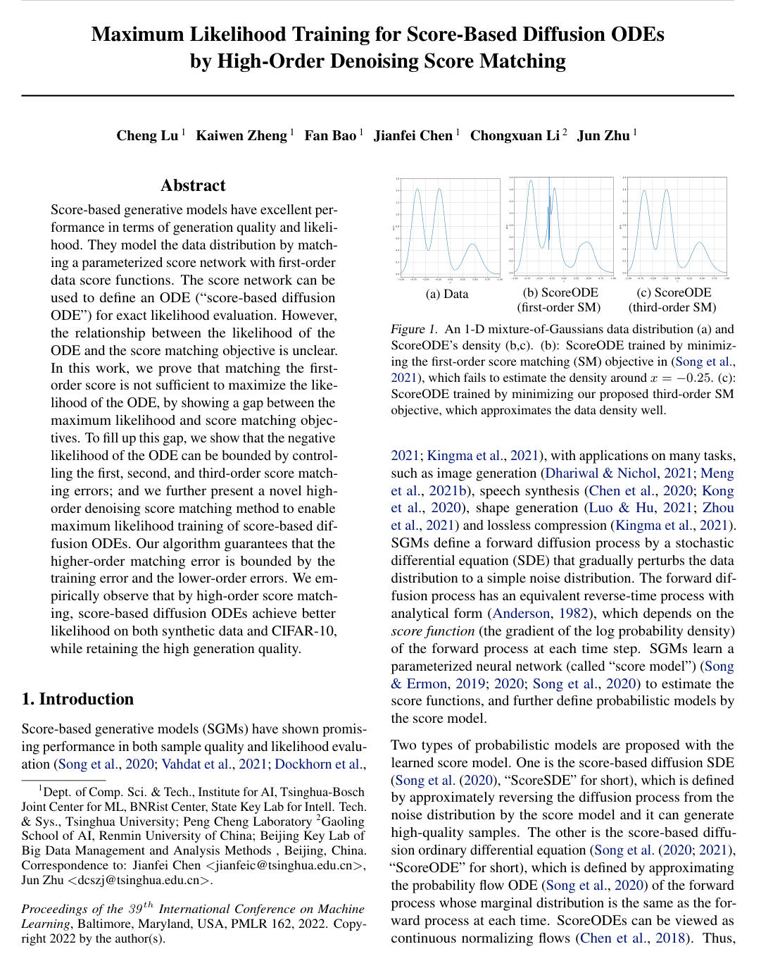
Score-based generative models have emerged as leading tools for creating high-fidelity images, audio, and complex synthetic data. These models operate through two primary mathematical representations: stochastic differential equations, which excel at generating realistic samples, and ordinary differential equations (diffusion ODEs), which enable exact evaluation of data likelihood for density estimation and model comparison. However, standard training procedures minimize only first-order score matching errors (matching the gradient of the log data distribution). While this maximizes the likelihood of the stochastic model, it does not guarantee high likelihood for the corresponding diffusion ODE, often resulting in severe density misestimations even on simple synthetic datasets.

The main objective of the article is to establish the theoretical relationship between score matching objectives and diffusion ODE likelihood, and to develop an error-bounded training method that directly maximizes ODE likelihood without sacrificing sample quality or computational scalability.

To address this objective, the authors conduct mathematical proofs to identify the gap between the Kullback-Leibler divergence (a standard measure of difference between probability distributions) and first-order score matching. They prove that ODE likelihood can be bounded by simultaneously controlling first-, second-, and third-order score matching errors (the gradient, Hessian, and gradient of the Hessian trace). Rather than using slow, step-by-step differential equation solvers during training, the authors introduce a scalable high-order denoising score matching algorithm that uses Monte Carlo random sampling and efficient trace estimators. They evaluate their method using synthetic 1-D and 2-D data distributions alongside benchmark image datasets (CIFAR-10 and ImageNet 32x32) using Variance Exploding diffusion models.

The key findings are structured as follows:

Theoretical Gap: Minimizing standard first-order score matching leaves an uncontrolled error term in the diffusion ODE's likelihood, explaining why previous models produced poor density estimates.
Error-Bounded Framework: The proposed high-order algorithm mathematically guarantees that higher-order score matching errors remain strictly bounded by lower-order errors and empirical training error.
Improved Likelihood: On CIFAR-10 image benchmarks, the method improves the negative log-likelihood of deep Variance Exploding models from 3.45 to 3.27 bits per dimension, and on ImageNet 32x32 from 4.21 to 4.03 bits per dimension.
Preserved Generation Quality: The model retains state-of-the-art sample quality (achieving competitive image quality scores of 2.61 vs. 2.19 on CIFAR-10) because the optimal model state remains aligned with the true data score function.
Practical Computational Overhead: The training method requires no expensive differential equation solvers; memory consumption and runtime remain practical, with third-order training running in less than double the time of standard first-order training.

These findings resolve a longstanding discrepancy between high sample quality and poor likelihood evaluation in diffusion models. By establishing bounded high-order score matching, the article provides a path to train generative models that are both top-tier data generators and reliable density estimators. This dual capability reduces technical risk in applications requiring rigorous probabilistic guarantees, such as anomaly detection, data compression, and uncertainty quantification.

For practical implementation, teams deploying diffusion models should consider fine-tuning existing pretrained model checkpoints with second- or third-order objectives rather than training from scratch, which converges in approximately 100,000 iterations (roughly half a day of compute). Practitioners should also adopt standard trace estimators and variance-reduction weighting to keep compute costs manageable. Future development should focus on extending these high-order principles to other diffusion architectures, including latent-space and critically-damped Langevin models.

The study's primary limitation is that near the starting time step (t close to zero), numerical instability and unbounded score errors can diminish likelihood gains on certain architecture types (such as Variance Preserving models). However, the theoretical framework is mathematically sound, and empirical results provide strong confidence in the effectiveness of high-order score matching for scalable, high-performing density modeling.

Department of Computer Science and Technology Peng Cheng Laboratory Renmin University of China Tsinghua-Bosch Joint ML Center Tsinghua University matching algorithm matching methods ordinary differential equations score-based diffusion ODEs high-order denoising score matching maximum likelihood training

arXiv: 2206.08265 LuChengTHU/mle_score_ode

Paper: Score-Based Generative Modeling through Stochastic Differential Equations, Yang Song et al. (2021). Introduces the continuous-time stochastic differential equation and probability flow ODE formulations of score-based diffusion models that this work directly analyzes and optimizes.
Paper: Estimation of Non-Normalized Statistical Models by Score Matching, Aapo Hyvärinen (2005). Establishes foundational score matching for non-normalized densities, providing the mathematical underpinning extended here to higher-order score derivatives.
Paper: Generative Modeling by Estimating Gradients of the Data Distribution, Yang Song et al. (2019). Pioneers noise-conditional score networks trained via denoising score matching, which this paper enhances through higher-order objectives.
Paper: Denoising Diffusion Probabilistic Models, Jonathan Ho et al. (2020). Connects discrete denoising diffusion probabilistic models to continuous score matching, establishing the base training framework examined in this paper.
Paper: Variational Diffusion Models, Diederik P. Kingma et al. (2021). Investigates likelihood estimation bounds in continuous-time diffusion models, highlighting the likelihood gap that higher-order score matching addresses.
Paper: Denoising Diffusion Implicit Models, Jiaming Song et al. (2021). Develops deterministic implicit sampling trajectories that correspond to continuous diffusion ODEs evaluated for exact likelihood computation.
Paper: Improved Techniques for Training Score-Based Generative Models, Yang Song et al. (2020). Provides key technical and architectural foundations for scaling variance-exploding score-based generative models.

Paper: Elucidating the Design Space of Diffusion-Based Generative Models, Tero Karras et al. (2022). Systematizes the design space of diffusion ODEs and deterministic higher-order solvers, complementing exact likelihood-driven ODE training.
Paper: Flow Matching for Generative Modeling, Yaron Lipman et al. (2023). Extends continuous ODE-based generative paths by directly matching continuous velocity fields rather than higher-order score gradients.
Paper: Consistency Models, Yang Song et al. (2023). Enforces consistency along probability flow ODE trajectories to enable rapid single- and few-step sampling from models trained via continuous ODE dynamics.
Paper: Stochastic Interpolants: A Unifying Framework for Flows and Diffusions, Michael S. Albergo et al. (2025). Unifies deterministic ODE flows and stochastic diffusions through finite-time interpolants, generalizing probability flow modeling.
Paper: Score-Based Diffusion Models in Function Space, Jae Hyun Lim 0001 et al. (2025). Extends score-based diffusion differential equation formulations from finite Euclidean spaces to infinite-dimensional function spaces.
Paper: A Mathematical Introduction to Diffusion Models, Jianfeng Lu (2026). Provides a comprehensive mathematical treatment of continuous reverse dynamics, discretization errors, and score-matching sample bounds.

Cover for Maximum Likelihood Training for Score-based Diffusion ODEs by High Order Denoising Score Matching

Abstract

Score-based generative models have excellent performance in terms of generation quality and likelihood. They model the data distribution by matching a parameterized score network with first-order data score functions. The score network can be used to define an ODE (“score-based diffusion ODE”) for exact likelihood evaluation. However, the relationship between the likelihood of the ODE and the score matching objective is unclear. In this work, we prove that matching the first-order score is not sufficient to maximize the likelihood of the ODE, by showing a gap between the maximum likelihood and score matching objectives. To fill up this gap, we show that the negative likelihood of the ODE can be bounded by controlling the first, second, and third-order score matching errors; and we further present a novel high-order denoising score matching method to enable maximum likelihood training of score-based diffusion ODEs. Our algorithm guarantees that the higher-order matching error is bounded by the training error and the lower-order errors. We empirically observe that by high-order score matching, score-based diffusion ODEs achieve better likelihood on both synthetic data and CIFAR-10, while retaining the high generation quality.

Topics

matching algorithm matching methods ordinary differential equations posterior probability maximum likelihood method

Keywords

score-based diffusion ODEs high-order denoising score matching maximum likelihood training second-order score matching objective probability flow ODE score function estimation diffusion models stochastic differential equations

1. Introduction
2. Score-Based Generative Models
2.1. ScoreSDEs and Maximum Likelihood Training
2.2. ScoreODEs and Exact Likelihood Evaluation
3. Relationship between Score Matching and KL Divergence of ScoreODEs
3.1. KL Divergence of ScoreODEs
3.2. Bounding the KL Divergence of ScoreODEs by High-Order Score Matching Errors
4. Error-Bounded High-Order Denoising Score Matching (DSM)
4.1. First-Order Denoising Score Matching
4.2. High-Order Denoising Score Matching
5. Training Score Models by High-Order DSM
5.1. Variance Reduction by Time-Reweighting
5.2. Scalability and Numerical Stability
6. Related Work
7. Experiments
7.1. Example: 1-D Mixture of Gaussians
7.2. Density Modeling on 2-D Checkerboard Data
7.3. Density Modeling on Image Datasets
8. Conclusion
Acknowledgements
References
A. Assumptions
B. Distribution gap between score-based diffusion SDEs and ODEs
C. KL divergence and variational gap of ScoreSDEs
D. Instantaneous change of score function of ODEs
E. KL divergence of ScoreODEs
E.1. Proof of Theorem 3.1
E.2. Proof of Theorem 3.2
E.3. Maximum likelihood training of ScoreODE by ODE solvers
F. Error-bounded High-Order Denoising Score Matching
F.1. Proof of Theorem 4.1
F.2. Proof of Corollary 4.2
F.3. Proof of Theorem 4.3
F.4. Difference between error-bounded high-order denoising score matching and previous high-order score matching in Meng et al. (2021a)
G. Estimated objectives of high-order DSM for high-dimensional data
G.1. Relationship between the estimated objectives and the original objectives for high-order DSM
H. Training algorithm
I. Experiment details
I.1. Choosing of λ 1 , λ 2
I.2. 1-D mixture of Gaussians
I.3. 2-D checkerboard data
I.4. CIFAR-10 experiments
I.5. ImageNet 32x32 experiments
J. Additional results for VE, VP and subVP types

Knowls

Knowl 1 — Decomposition of KL Divergence for Score-Based Diffusion ODEs
theoretical result
Let $q_0(x_0)$ be an unknown $d$ -dimensional data distribution, and consider the forward diffusion stochastic differential equation (SDE): $dx_t = f(x_t, t)dt + g(t)dw_t, \quad t \in [0, T]$ where $f(\cdot, t): \mathbb{R}^d \to \mathbb{R}^d$ , $g(t) \in \mathbb{R}$ , $w_t$ is a standard Wiener process, and $q_t(x_t)$ is the marginal distribution at time $t$ . The ScoreODE associated with a parameterized score model $s_\theta(x_t, t)$ is defined by: $\frac{dx_t}{dt} = f(x_t, t) - \frac{1}{2}g(t)^2 s_\theta(x_t, t)$ with marginal distribution $p_t^{\mathrm{ODE}}(x_t)$ and terminal distribution $p_T^{\mathrm{ODE}}(x_T) = \mathcal{N}(x_T \mid 0, \sigma_T^2 I)$ .

Under regularity conditions, the KL divergence between $q_0$ and $p_0^{\mathrm{ODE}}$ decomposes as: $D_{\mathrm{KL}}(q_0 \parallel p_0^{\mathrm{ODE}}) = D_{\mathrm{KL}}(q_T \parallel p_T^{\mathrm{ODE}}) + J_{\mathrm{SM}}(\theta) + J_{\mathrm{Diff}}(\theta)$ where: $J_{\mathrm{SM}}(\theta) = \frac{1}{2} \int_0^T g(t)^2 \mathbb{E}_{q_t(x_t)}\left[ \|s_\theta(x_t, t) - \nabla_x \log q_t(x_t)\|_2^2 \right] dt$ $J_{\mathrm{Diff}}(\theta) = \frac{1}{2} \int_0^T g(t)^2 \mathbb{E}_{q_t(x_t)}\left[ (s_\theta(x_t, t) - \nabla_x \log q_t(x_t))^\top (\nabla_x \log p_t^{\mathrm{ODE}}(x_t) - s_\theta(x_t, t)) \right] dt$

While $J_{\mathrm{SM}}(\theta)$ bounds the KL divergence of the parameterized ScoreSDE ( $D_{\mathrm{KL}}(q_0 \parallel p_0^{\mathrm{SDE}}) \le D_{\mathrm{KL}}(q_T \parallel p_T^{\mathrm{SDE}}) + J_{\mathrm{SM}}(\theta)$ ), minimizing $J_{\mathrm{SM}}(\theta)$ alone does not minimize $D_{\mathrm{KL}}(q_0 \parallel p_0^{\mathrm{ODE}})$ due to the presence of $J_{\mathrm{Diff}}(\theta)$ , which depends on the model's instantaneous score $\nabla_x \log p_t^{\mathrm{ODE}}(x_t)$ .
Knowl 2 — Upper Bound on ScoreODE Fisher Divergence via High-Order Score Errors
theoretical result
Let $D_{\mathrm{F}}(q \parallel p) = \mathbb{E}_{q(x)}[\|\nabla_x \log p(x) - \nabla_x \log q(x)\|_2^2]$ denote the Fisher divergence between distributions $q$ and $p$ . In the KL divergence decomposition $D_{\mathrm{KL}}(q_0 \parallel p_0^{\mathrm{ODE}}) = D_{\mathrm{KL}}(q_T \parallel p_T^{\mathrm{ODE}}) + J_{\mathrm{ODE}}(\theta)$ where $J_{\mathrm{ODE}}(\theta) = J_{\mathrm{SM}}(\theta) + J_{\mathrm{Diff}}(\theta)$ , applying the Cauchy-Schwarz inequality yields: $J_{\mathrm{ODE}}(\theta) \le \sqrt{J_{\mathrm{SM}}(\theta)} \cdot \sqrt{J_{\mathrm{Fisher}}(\theta)}$ where $J_{\mathrm{Fisher}}(\theta) = \frac{1}{2} \int_0^T g(t)^2 D_{\mathrm{F}}(q_t \parallel p_t^{\mathrm{ODE}}) dt$ .

Assume there exists $C > 0$ such that $\|\nabla_x^2 \log p_t^{\mathrm{ODE}}(x_t)\|_2 \le C$ for all $t \in [0, T]$ and $x_t \in \mathbb{R}^d$ (where $\|\cdot\|_2$ is the spectral norm), and assume that the score network $s_\theta(x_t, t)$ satisfies uniform error bounds: $\|s_\theta(x_t, t) - \nabla_x \log q_t(x_t)\|_2 \le \delta_1$ $\|\nabla_x s_\theta(x_t, t) - \nabla_x^2 \log q_t(x_t)\|_F \le \delta_2$ $\|\nabla_x \operatorname{tr}(\nabla_x s_\theta(x_t, t)) - \nabla_x \operatorname{tr}(\nabla_x^2 \log q_t(x_t))\|_2 \le \delta_3$ where $\|\cdot\|_F$ is the Frobenius norm. Then there exists an upper bound $U(t; \delta_1, \delta_2, \delta_3, C, q) \ge 0$ independent of $\theta$ such that: $D_{\mathrm{F}}(q_t \parallel p_t^{\mathrm{ODE}}) \le U(t; \delta_1, \delta_2, \delta_3, C, q)$ For all $t \in [0, T]$ with $g(t) \neq 0$ , $U$ is strictly increasing in $\delta_1, \delta_2,$ and $\delta_3$ . Thus, bounding first, second, and third-order score errors bounds $J_{\mathrm{Fisher}}(\theta)$ and consequently $D_{\mathrm{KL}}(q_0 \parallel p_0^{\mathrm{ODE}})$ .
Knowl 3 — Error-Bounded Second-Order Denoising Score Matching
theoretical result
Let the forward diffusion process satisfy the Gaussian transition $q(x_t \mid x_0) = \mathcal{N}(x_t \mid \alpha_t x_0, \sigma_t^2 I)$ for scalar coefficients $\alpha_t \in \mathbb{R}, \sigma_t > 0$ . Let $\hat{s}_1(x_t, t)$ be an estimation of the first-order score $\nabla_x \log q_t(x_t)$ with point-wise error $\delta_1(x_t, t) := \|\hat{s}_1(x_t, t) - \nabla_x \log q_t(x_t)\|_2$ .

A second-order matrix score model $s_2(\cdot, t; \theta): \mathbb{R}^d \to \mathbb{R}^{d \times d}$ estimating the Hessian $\nabla_x^2 \log q_t(x_t)$ is learned by solving: $\theta^* = \arg\min_\theta \mathbb{E}_{x_0 \sim q_0, \epsilon \sim \mathcal{N}(0, I)}\left[ \frac{1}{\sigma_t^4} \left\| \sigma_t^2 s_2(x_t, t; \theta) + I - \ell_1 \ell_1^\top \right\|_F^2 \right]$ where $x_t = \alpha_t x_0 + \sigma_t \epsilon$ and $\ell_1(\epsilon, x_0, t) := \sigma_t \hat{s}_1(x_t, t) + \epsilon$ .

For any $x_t$ and parameter $\theta$ , the second-order estimation error satisfies the deterministic bound: $\|s_2(x_t, t; \theta) - \nabla_x^2 \log q_t(x_t)\|_F \le \|s_2(x_t, t; \theta) - s_2(x_t, t; \theta^*)\|_F + \delta_1(x_t, t)^2$ where $\|s_2(x_t, t; \theta) - s_2(x_t, t; \theta^*)\|_F$ is the surrogate training error.
Knowl 4 — Error-Bounded Second-Order Trace Denoising Score Matching
theoretical result
For a forward diffusion process with Gaussian transition $q(x_t \mid x_0) = \mathcal{N}(x_t \mid \alpha_t x_0, \sigma_t^2 I)$ and a first-order score estimate $\hat{s}_1(x_t, t)$ having error $\delta_1(x_t, t) = \|\hat{s}_1(x_t, t) - \nabla_x \log q_t(x_t)\|_2$ , a scalar trace score model $s_2^{\mathrm{trace}}(\cdot, t; \theta): \mathbb{R}^d \to \mathbb{R}$ targeting $\operatorname{tr}(\nabla_x^2 \log q_t(x_t))$ is trained by solving: $\theta^* = \arg\min_\theta \mathbb{E}_{x_0 \sim q_0, \epsilon \sim \mathcal{N}(0, I)}\left[ \frac{1}{\sigma_t^4} \left| \sigma_t^2 s_2^{\mathrm{trace}}(x_t, t; \theta) + d - \|\ell_1\|_2^2 \right|^2 \right]$ where $d$ is the data dimension, $x_t = \alpha_t x_0 + \sigma_t \epsilon$ , and $\ell_1 = \sigma_t \hat{s}_1(x_t, t) + \epsilon$ .

The estimation error for $s_2^{\mathrm{trace}}$ is bounded by: $\left| s_2^{\mathrm{trace}}(x_t, t; \theta) - \operatorname{tr}(\nabla_x^2 \log q_t(x_t)) \right| \le \left| s_2^{\mathrm{trace}}(x_t, t; \theta) - s_2^{\mathrm{trace}}(x_t, t; \theta^*) \right| + \delta_1(x_t, t)^2$
Knowl 5 — Error-Bounded Third-Order Denoising Score Matching
theoretical result
Let $\hat{s}_1(x_t, t)$ estimate $\nabla_x \log q_t(x_t)$ with error $\delta_1(x_t, t)$ , and let $\hat{s}_2(x_t, t)$ estimate $\nabla_x^2 \log q_t(x_t)$ with errors $\delta_2(x_t, t) := \|\hat{s}_2(x_t, t) - \nabla_x^2 \log q_t(x_t)\|_F$ and $\delta_{2,\mathrm{tr}}(x_t, t) := |\operatorname{tr}(\hat{s}_2(x_t, t)) - \operatorname{tr}(\nabla_x^2 \log q_t(x_t))|$ .

A third-order vector score model $s_3(\cdot, t; \theta): \mathbb{R}^d \to \mathbb{R}^d$ estimating $\nabla_x \operatorname{tr}(\nabla_x^2 \log q_t(x_t))$ is trained by minimizing: $\theta^* = \arg\min_\theta \mathbb{E}_{x_0 \sim q_0, \epsilon \sim \mathcal{N}(0, I)}\left[ \frac{1}{\sigma_t^6} \left\| \sigma_t^3 s_3(x_t, t; \theta) + \ell_3 \right\|_2^2 \right]$ where $x_t = \alpha_t x_0 + \sigma_t \epsilon$ , and the auxiliary variables are defined by: $\ell_1 := \sigma_t \hat{s}_1(x_t, t) + \epsilon$ $\ell_2 := \sigma_t^2 \hat{s}_2(x_t, t) + I$ $\ell_3 := \left( \|\ell_1\|_2^2 I - \operatorname{tr}(\ell_2)I - 2\ell_2 \right) \ell_1$

For any $x_t$ and $\theta$ , the third-order estimation error satisfies: $\|s_3(x_t, t; \theta) - \nabla_x \operatorname{tr}(\nabla_x^2 \log q_t(x_t))\|_2 \le \|s_3(x_t, t; \theta) - s_3(x_t, t; \theta^*)\|_2 + \left( \delta_1(x_t, t)^2 + \delta_{2,\mathrm{tr}}(x_t, t) + 2\delta_2(x_t, t) \right) \delta_1(x_t, t)$
Knowl 6 — Scalable High-Order DSM Training Algorithm with Trace Estimators
algorithm
To train a neural network score model $s_\theta(x, t)$ via high-order denoising score matching on high-dimensional data without $O(d^2)$ matrix operations, Hutchinson's trace estimator with random vector $v \sim p(v)$ (with $\mathbb{E}[v]=0$ and $\operatorname{Cov}[v]=I$ , such as standard Gaussian or Rademacher) is combined with forward-mode Jacobian-vector products (JVP) and reverse-mode vector-Jacobian products (VJP).

The time-reweighted multi-order loss optimized over $t \sim \mathcal{U}(\epsilon, T)$ is: $\min_\theta \mathcal{J}_{\mathrm{DSM}}^{(1)}(\theta) + \lambda_1 \left( \mathcal{J}_{\mathrm{DSM, est}}^{(2)}(\theta) + \mathcal{J}_{\mathrm{DSM, est}}^{(2,\mathrm{tr})}(\theta) \right) + \lambda_2 \mathcal{J}_{\mathrm{DSM, est}}^{(3)}(\theta)$ where gradients through the lower-order score estimates $\hat{s}_1 = \text{stop\_gradient}(s_\theta(x_t, t))$ and $\hat{s}_{\mathrm{jvp}} = \text{stop\_gradient}(\nabla_x s_\theta(x_t, t)v)$ are detached.
Input: Score network $s_\theta$ , hyperparameters $\lambda_1, \lambda_2$ , minimum time $\epsilon$ , forward process schedules $\alpha_t, \sigma_t$ , data sample $x_0 \sim q_0(x_0)$ .
Output: Denoising score matching loss $\mathcal{J}_{\mathrm{DSM}}(\theta)$ .
Sample $\epsilon \sim \mathcal{N}(0, I)$
Sample $v \sim \mathcal{N}(0, I)$ or Rademacher $(\pm 1)$
Sample $t \sim \mathcal{U}(\epsilon, T)$
Compute $x_t \leftarrow \alpha_t x_0 + \sigma_t \epsilon$
Compute $s_\theta(x_t, t)$ and $s_{\mathrm{jvp}} \leftarrow \nabla_x s_\theta(x_t, t)v$ using forward-mode autodiff (JVP)
Compute $v^\top \nabla_x s_{\mathrm{jvp}}$ using reverse-mode autodiff (VJP)
Set $\hat{s}_1 \leftarrow \text{stop\_gradient}(s_\theta(x_t, t))$
Set $\hat{s}_{\mathrm{jvp}} \leftarrow \text{stop\_gradient}(s_{\mathrm{jvp}})$
Compute $\mathcal{J}_{\mathrm{DSM}}^{(1)}(\theta) \leftarrow \|\sigma_t s_\theta(x_t, t) + \epsilon\|_2^2$
Compute $\mathcal{J}_{\mathrm{DSM, est}}^{(2)}(\theta) \leftarrow \|\sigma_t^2 s_{\mathrm{jvp}} + v - (\sigma_t \hat{s}_1 \cdot v + \epsilon \cdot v)(\sigma_t \hat{s}_1 + \epsilon)\|_2^2$
Compute $\mathcal{J}_{\mathrm{DSM, est}}^{(2,\mathrm{tr})}(\theta) \leftarrow |\sigma_t^2 v^\top s_{\mathrm{jvp}} + \|v\|_2^2 - |\sigma_t \hat{s}_1 \cdot v + \epsilon \cdot v|^2|^2$
Compute $\ell_3(v) \leftarrow |\sigma_t \hat{s}_1 \cdot v + \epsilon \cdot v|^2(\sigma_t \hat{s}_1 + \epsilon) - (\sigma_t^2 v^\top \hat{s}_{\mathrm{jvp}} + \|v\|_2^2)(\sigma_t \hat{s}_1 + \epsilon) - 2(\sigma_t \hat{s}_1 \cdot v + \epsilon \cdot v)(\sigma_t^2 \hat{s}_{\mathrm{jvp}} + v)$
Compute $\mathcal{J}_{\mathrm{DSM, est}}^{(3)}(\theta) \leftarrow \|\sigma_t^3 v^\top \nabla_x s_{\mathrm{jvp}} + \ell_3(v)\|_2^2$
return $\mathcal{J}_{\mathrm{DSM}}^{(1)}(\theta) + \lambda_1 (\mathcal{J}_{\mathrm{DSM, est}}^{(2)}(\theta) + \mathcal{J}_{\mathrm{DSM, est}}^{(2,\mathrm{tr})}(\theta)) + \lambda_2 \mathcal{J}_{\mathrm{DSM, est}}^{(3)}(\theta)$
Knowl 7 — Instantaneous Change of Score Function for ODEs
theoretical result
Let $z(t) \in \mathbb{R}^d$ be a continuous random variable with probability density $p(z(t), t)$ driven by the ordinary differential equation: $\frac{dz(t)}{dt} = f(z(t), t)$ Assuming $f \in C^3(\mathbb{R}^{d+1})$ , the instantaneous score function $\nabla_z \log p(z(t), t)$ evolves along the ODE trajectory according to the total derivative: $\frac{d \nabla_z \log p(z(t), t)}{dt} = -\nabla_z \left( \operatorname{tr}(\nabla_z f(z(t), t)) \right) - (\nabla_z f(z(t), t))^\top \nabla_z \log p(z(t), t)$

This differential equation allows computing the exact score $\nabla_x \log p_0^{\mathrm{ODE}}(x_0)$ of a ScoreODE by first integrating $\frac{dx_t}{dt} = h_p(x_t, t)$ forward from $t=0$ to $t=T$ to obtain $x_T$ , and then integrating the augmented reverse system $(x_t, \nabla_x \log p_t^{\mathrm{ODE}}(x_t))$ from $t=T$ back to $t=0$ starting with initial condition $(x_T, \nabla_x \log p_T^{\mathrm{ODE}}(x_T))$ .
Knowl 8 — Distribution Discrepancy Between ScoreSDE and ScoreODE Dynamics
theoretical result
For a forward SDE $dx_t = f(x_t, t)dt + g(t)dw_t$ with linear drift $f(x_t, t) = \alpha(t)x_t$ , the probability flow ODE associated with the reverse ScoreSDE $dx_t = [f(x_t, t) - g(t)^2 s_\theta(x_t, t)]dt + g(t)d\bar{w}_t$ is given by: $\frac{dx_t}{dt} = f(x_t, t) - g(t)^2 s_\theta(x_t, t) + \frac{1}{2}g(t)^2 \nabla_x \log p_t^{\mathrm{SDE}}(x_t)$ which differs in form from the ScoreODE $\frac{dx_t}{dt} = f(x_t, t) - \frac{1}{2}g(t)^2 s_\theta(x_t, t)$ .

If $s_\theta(x_t, t) \equiv \nabla_x \log p_t^{\mathrm{SDE}}(x_t)$ for all $x_t \in \mathbb{R}^d$ and $t \in [0, T]$ , then by the Fokker-Planck equation and Cramér's decomposition theorem, $p_t^{\mathrm{SDE}}$ is necessarily a Gaussian distribution for all $t \in [0, T]$ . Since non-trivial data distributions $q_0$ are non-Gaussian, $s_\theta(x_t, t) \neq \nabla_x \log p_t^{\mathrm{SDE}}(x_t)$ must hold at some $t$ , implying $p_0^{\mathrm{SDE}} \neq p_0^{\mathrm{ODE}}$ in practice. Consequently, maximizing the likelihood of $p_0^{\mathrm{SDE}}$ via first-order score matching does not maximize the likelihood of the ScoreODE $p_0^{\mathrm{ODE}}$ .

Knowl 9 — Quantitative Likelihood and Generation Quality on CIFAR-10 and ImageNet 32x32

data/table

Continuous score-based diffusion models of Variance Exploding (VE) type evaluated on CIFAR-10 and ImageNet $32\times 32$ show that incorporating high-order denoising score matching systematically improves the negative log-likelihood (NLL, measured in bits per dimension / bpd) of the ScoreODE while retaining the sample quality (FID score) of the ScoreSDE using the Predictor-Corrector (PC) sampler.

Model	CIFAR-10		ImageNet $32\times 32$
	NLL (bpd) $\downarrow$	FID $\downarrow$	NLL (bpd) $\downarrow$
VE (Song et al., 2020)	3.66	2.42	4.21
VE (second-order DSM)	3.44	2.37	4.06
VE (third-order DSM)	3.38	2.95	4.04
VE deep (Song et al., 2020)	3.45	2.19	4.21
VE deep (second-order DSM)	3.35	2.43	4.05
VE deep (third-order DSM)	3.27	2.61	4.03

Likelihood is evaluated exactly via uniform dequantization and ODE integration down to $\epsilon = 10^{-5}$ across test sets (averaged over 5 repetitions of trace estimation); FID is evaluated using 50k samples generated from the reverse SDE with 1000 steps. Third-order DSM reduces CIFAR-10 bpd from 3.66 to 3.38 (and 3.45 to 3.27 for deep VE) while maintaining FID below 3.0.

Knowl 10 — Error Propagation Comparison with Previous High-Order DSM Formulations
theoretical result
In the second-order denoising score matching objective proposed by Meng et al. (2021a): $\theta^* = \arg\min_\theta \mathbb{E}_{q_t, q_{t0}}\left[ \left\| s_2(\theta) - \nabla_x^2 \log q(x_t \mid x_0) - \nabla_x \log q(x_t \mid x_0)\nabla_x \log q(x_t \mid x_0)^\top + \hat{s}_1 \hat{s}_1^\top \right\|_F^2 \right]$ the optimal model Hessian satisfies: $s_2(\theta^*) - \nabla_x^2 \log q_t(x_t) = \nabla_x \log q_t(x_t)\nabla_x \log q_t(x_t)^\top - \hat{s}_1(x_t, t)\hat{s}_1(x_t, t)^\top$ If $\hat{s}_1(x_t, t) - \nabla_x \log q_t(x_t) = \delta_1 \mathbf{1}$ and the data score $\nabla_x \log q_t(x_t)$ is unbounded, the estimation error satisfies: $\|s_2(\theta^*) - \nabla_x^2 \log q_t(x_t)\|_F \ge 2\delta_1 \|\nabla_x \log q_t(x_t)\|_2 - \delta_1^2 d$ which can be arbitrarily large for any small $\delta_1 > 0$ when the true score is large.

In contrast, the error-bounded second-order DSM objective guarantees that: $\|s_2(\theta^*) - \nabla_x^2 \log q_t(x_t)\|_F = \|\hat{s}_1(x_t, t) - \nabla_x \log q_t(x_t)\|_2^2 = \delta_1(x_t, t)^2$ ensuring that the second-order score error is strictly upper bounded by the squared first-order error regardless of the magnitude of the score function.

Knowl 11 — Computational Overhead of High-Order Score Matching Training

data/table

Empirical runtime and GPU memory consumption benchmarks measured on CIFAR-10 using 8 NVIDIA GeForce RTX 2080 Ti GPUs (batch size 48) demonstrate the scalability of high-order DSM via automatic differentiation:

Second-order DSM training adds only +17.8% runtime and +12.0% memory overhead relative to standard first-order score matching. Third-order DSM costs less than double the per-iteration time (+57.1%) and converges rapidly when fine-tuning from pre-trained first-order checkpoints.

Knowl 12 — Start-Time Sensitivity and Unbounded Score Limitation in VP and subVP SDEs
limitation
When applying high-order denoising score matching to Variance Preserving (VP) and sub-Variance Preserving (subVP) SDEs, the method reduces negative log-likelihood for moderately small starting times $\epsilon$ (e.g., $\epsilon \ge 10^{-3}$ on CIFAR-10), but fails to improve likelihood when $\epsilon$ is pushed close to zero (e.g., $\epsilon = 10^{-5}$ ).

This limitation arises from the unbounded score problem near $t = 0$ in VP and subVP diffusions, where first-order score matching error diverges near $t=0$ , causing high-order surrogate targets to lose efficacy. In contrast, the score singularity near $t = 0$ in Variance Exploding (VE) diffusions is much milder, allowing high-order DSM to achieve substantial ScoreODE likelihood improvements across all tested evaluation thresholds down to $\epsilon = 10^{-5}$ .

Coverage note — None was omitted; all main theoretical bounds, algorithms, empirical evaluations, error comparisons, and documented limitations are covered.

References

1.Anderson, B. D. Reverse-time diffusion equation models. Stochastic Processes and their Applications, 12(3):313–326, 1982.
2.Bradbury, J., Frostig, R., Hawkins, P., Johnson, M. J., Leary, C., Maclaurin, D., Necula, G., Paszke, A., VanderPlas, J., Wanderman-Milne, S., and Zhang, Q. JAX: Composable transformations of Python+NumPy programs, 2018. URL http://github.com/google/jax.
3.Chen, N., Zhang, Y., Zen, H., Weiss, R. J., Norouzi, M., and Chan, W. Wavegrad: Estimating gradients for waveform generation. arXiv preprint arXiv:2009.00713, 2020.
4.Chen, R. T., Rubanova, Y., Bettencourt, J., and Duvenaud, D. Neural ordinary differential equations. arXiv preprint arXiv:1806.07366, 2018.
5.Deng, J., Dong, W., Socher, R., Li, L., Li, K., and Fei-Fei, L. ImageNet: A large-scale hierarchical image database. In 2009 IEEE Conference on Computer Vision and Pattern Recognition, pp. 248–255. IEEE, 2009.
6.Dhariwal, P. and Nichol, A. Diffusion models beat GANs on image synthesis. arXiv preprint arXiv:2105.05233, 2021.
7.Dockhorn, T., Vahdat, A., and Kreis, K. Score-based generative modeling with critically-damped langevin diffusion. arXiv preprint arXiv:2112.07068, 2021.
8.Finlay, C., Jacobsen, J.-H., Nurbekyan, L., and Oberman, A. How to train your Neural ODE: the world of Jacobian and kinetic regularization. In International Conference on Machine Learning, pp. 3154–3164. PMLR, 2020.
9.Grathwohl, W., Chen, R. T., Bettencourt, J., Sutskever, I., and Duvenaud, D. FFJORD: Free-form continuous dynamics for scalable reversible generative models. arXiv preprint arXiv:1810.01367, 2018.
10.Ho, J., Jain, A., and Abbeel, P. Denoising diffusion probabilistic models. arXiv preprint arXiv:2006.11239, 2020.
11.Huang, C.-W., Lim, J. H., and Courville, A. A variational perspective on diffusion-based generative models and score matching. arXiv preprint arXiv:2106.02808, 2021.
12.Hutchinson, M. F. A stochastic estimator of the trace of the influence matrix for Laplacian smoothing splines. Communications in Statistics-Simulation and Computation, 18(3):1059–1076, 1989.
13.Hyv¨arinen, A. and Dayan, P. Estimation of non-normalized statistical models by score matching. Journal of Machine Learning Research, 6(4), 2005.
14.Kingma, D. P. and Ba, J. Adam: A method for stochastic optimization. arXiv preprint arXiv:1412.6980, 2014.
15.Kingma, D. P., Salimans, T., Poole, B., and Ho, J. Variational diffusion models. arXiv preprint arXiv:2107.00630, 2021.
16.Kong, Z., Ping, W., Huang, J., Zhao, K., and Catanzaro, B. Diffwave: A versatile diffusion model for audio synthesis. arXiv preprint arXiv:2009.09761, 2020.
17.Krizhevsky, A. Learning multiple layers of features from tiny images. Technical report, 2009.
18.Luo, S. and Hu, W. Diffusion probabilistic models for 3D point cloud generation. In Proceedings of the IEEE/CVF Conference on Computer Vision and Pattern Recognition, pp. 2837–2845, 2021.
19.Meng, C., Song, Y., Li, W., and Ermon, S. Estimating high order gradients of the data distribution by denoising. Advances in Neural Information Processing Systems, 34, 2021a.
20.Meng, C., Song, Y., Song, J., Wu, J., Zhu, J.-Y., and Ermon, S. SDEdit: Image synthesis and editing with stochastic differential equations. arXiv preprint arXiv:2108.01073, 2021b.
21.Ramachandran, P., Zoph, B., and Le, Q. V. Searching for activation functions. arXiv preprint arXiv:1710.05941, 2017.
22.Skilling, J. The eigenvalues of mega-dimensional matrices. In Maximum Entropy and Bayesian Methods, pp. 455–466. Springer, 1989.
23.Song, Y. and Ermon, S. Generative modeling by estimating gradients of the data distribution. arXiv preprint arXiv:1907.05600, 2019.
24.Song, Y. and Ermon, S. Improved techniques for training score-based generative models. arXiv preprint arXiv:2006.09011, 2020.
25.Song, Y., Sohl-Dickstein, J., Kingma, D. P., Kumar, A., Ermon, S., and Poole, B. Score-based generative modeling through stochastic differential equations. arXiv preprint arXiv:2011.13456, 2020.
26.Song, Y., Durkan, C., Murray, I., and Ermon, S. Maximum likelihood training of score-based diffusion models. arXiv e-prints, pp. arXiv–2101, 2021.
27.Vahdat, A., Kreis, K., and Kautz, J. Score-based generative modeling in latent space. arXiv preprint arXiv:2106.05931, 2021.
28.Vincent, P. A connection between score matching and denoising autoencoders. Neural computation, 23(7):1661–1674, 2011.
29.Zhou, L., Du, Y., and Wu, J. 3D shape generation and completion through point-voxel diffusion. arXiv preprint arXiv:2104.03670, 2021.

Citation

MLA

Lu, C., et al. “Maximum Likelihood Training for Score-based Diffusion ODEs by High Order Denoising Score Matching”. International Conference on Machine Learning, vol. 162, 2022, pp. 14429–60, https://proceedings.mlr.press/v162/lu22f.html.

APA

Lu, C., Zheng, K., Bao, F., Chen, J., Li, C., & Zhu, J. (2022). Maximum Likelihood Training for Score-based Diffusion ODEs by High Order Denoising Score Matching. International Conference on Machine Learning, 162, 14429–14460. https://proceedings.mlr.press/v162/lu22f.html

Chicago

Lu, C., K. Zheng, F. Bao, J. Chen, C. Li, and J. Zhu. 2022. “Maximum Likelihood Training for Score-based Diffusion ODEs by High Order Denoising Score Matching”. International Conference on Machine Learning 162: 14429–60. https://proceedings.mlr.press/v162/lu22f.html.

Harvard

Lu, C. et al. (2022) “Maximum Likelihood Training for Score-based Diffusion ODEs by High Order Denoising Score Matching”, International Conference on Machine Learning. PMLR, pp. 14429–14460. Available at: https://proceedings.mlr.press/v162/lu22f.html.

Vancouver

1. Lu C, Zheng K, Bao F, Chen J, Li C, Zhu J (2022) Maximum Likelihood Training for Score-based Diffusion ODEs by High Order Denoising Score Matching. In: International Conference on Machine Learning. PMLR, pp 14429–14460

BibTeX

@InProceedings{pmlr-v162-lu22f,
  title = 	 {Maximum Likelihood Training for Score-based Diffusion {ODE}s by High Order Denoising Score Matching},
  author =       {Lu, Cheng and Zheng, Kaiwen and Bao, Fan and Chen, Jianfei and Li, Chongxuan and Zhu, Jun},
  booktitle = 	 {Proceedings of the 39th International Conference on Machine Learning},
  pages = 	 {14429--14460},
  year = 	 {2022},
  editor = 	 {Chaudhuri, Kamalika and Jegelka, Stefanie and Song, Le and Szepesvari, Csaba and Niu, Gang and Sabato, Sivan},
  volume = 	 {162},
  series = 	 {Proceedings of Machine Learning Research},
  month = 	 {17--23 Jul},
  publisher =    {PMLR},
  pdf = 	 {https://proceedings.mlr.press/v162/lu22f/lu22f.pdf},
  url = 	 {https://proceedings.mlr.press/v162/lu22f.html},
  abstract = 	 {Score-based generative models have excellent performance in terms of generation quality and likelihood. They model the data distribution by matching a parameterized score network with first-order data score functions. The score network can be used to define an ODE (“score-based diffusion ODE”) for exact likelihood evaluation. However, the relationship between the likelihood of the ODE and the score matching objective is unclear. In this work, we prove that matching the first-order score is not sufficient to maximize the likelihood of the ODE, by showing a gap between the maximum likelihood and score matching objectives. To fill up this gap, we show that the negative likelihood of the ODE can be bounded by controlling the first, second, and third-order score matching errors; and we further present a novel high-order denoising score matching method to enable maximum likelihood training of score-based diffusion ODEs. Our algorithm guarantees that the higher-order matching error is bounded by the training error and the lower-order errors. We empirically observe that by high-order score matching, score-based diffusion ODEs achieve better likelihood on both synthetic data and CIFAR-10, while retaining the high generation quality.}
}

Metadata:DOI registry

Source Code

This paper has an official code repository available. Click below to access the source code.

View Repository

Access the Paper

This paper is available from its original source. Click below to access the PDF.

Open PDF

License: https://creativecommons.org/licenses/by/4.0/

Model	Time / iteration (s)	Peak Memory (GiB)	Training iterations
VE (first-order)	0.28	25.84	1200k
VE (second-order)	0.33	28.93	1200k + 100k
VE (third-order)	0.44	49.12	1200k + 100k

Maximum Likelihood Training for Score-based Diffusion ODEs by High Order Denoising Score Matching

Abstract

Topics

Keywords

Table of Contents

Knowls

Knowl 1 — Decomposition of KL Divergence for Score-Based Diffusion ODEs

Knowl 2 — Upper Bound on ScoreODE Fisher Divergence via High-Order Score Errors

Knowl 3 — Error-Bounded Second-Order Denoising Score Matching

Knowl 4 — Error-Bounded Second-Order Trace Denoising Score Matching

Knowl 5 — Error-Bounded Third-Order Denoising Score Matching

Knowl 6 — Scalable High-Order DSM Training Algorithm with Trace Estimators

Knowl 7 — Instantaneous Change of Score Function for ODEs

Knowl 8 — Distribution Discrepancy Between ScoreSDE and ScoreODE Dynamics