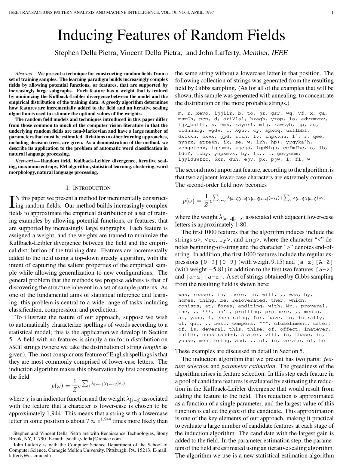
Inducing Features of Random Fields

Stephen Della PietraVincent J. Della PietraJ. Lafferty

article1995TPAMI1,355 citations

Introduces a principled framework for incrementally inducing complex features in random fields via maximum entropy and introduces the Improved Iterative Scaling algorithm to train non-Markovian exponential models with thousands of parameters.

Listen

Statistical learning models often struggle when dealing with rare events and high-dimensional data, such as natural language processing tasks where specific words appear only once in large corpora. The article introduces a method for automatically discovering structure from sample data by incrementally building non-Markovian random fields with thousands of parameters. The primary objective is to evaluate and demonstrate an incremental feature induction framework that constructs exponential probability models and estimates their parameters by minimizing relative entropy with respect to empirical training data.

The approach operates in two alternating stages: greedy feature selection and parameter estimation. During feature selection, candidate features are evaluated in parallel by estimating their potential information gain while holding other parameters fixed. The best candidate is added, and all model parameters are then re-estimated using Improved Iterative Scaling, a new algorithm that removes standard constraints and guarantees convergence via auxiliary functions. For large configuration spaces where exact summation is intractable, the approach computes expectations using Monte Carlo Gibbs sampling.

The evaluation yields several important findings. First, the greedy gain approximation allows the simultaneous evaluation of thousands of candidate features efficiently. Second, Improved Iterative Scaling guarantees monotonic convergence to the optimal maximum entropy distribution without requiring features to sum to a constant. Third, when applied to English word morphology across a 100,000-word vocabulary, the model progressively discovered foundational spelling rules—starting from basic lowercase characters, progressing to affixes like '-ed' and '-ion' across 100 features, and capturing complex structural regularities and macro symbols by 1,500 features.

These results demonstrate that feature induction can mitigate data sparsity and small-count problems by learning shared, sub-structural patterns rather than treating complex entities as atomic units. This improves modeling accuracy and generalization for downstream tasks such as word clustering and classification without relying on rigid probabilistic automata or restrictive Markovian assumptions.

To apply this approach, practitioners should consider incorporating batches of candidate features per iteration or delaying full parameter re-estimation to reduce computational overhead. Further work is required to develop principled Bayesian priors over candidate features to establish robust stopping criteria. Confidence in the mathematical foundation and convergence of the parameter estimation algorithm is high, though caution is warranted regarding computational scalability in higher-dimensional domains such as large-scale image processing, where Monte Carlo sampling of high-degree polynomials may become difficult.

Carnegie Mellon University Renaissance Technologies computer vision decision trees demonstrations feature induction random fields feature selection

arXiv: cmp-lg/9506014

Paper: Markov Random Field Texture Models, G. R. Cross et al. (1983). It provides foundational background on generative Markov-Gibbs random field models and parameter estimation for spatial interactions that the source paper contrasts against and extends to non-Markovian random fields.
Paper: A Bayesian method for the induction of probabilistic networks from data, Gregory F. Cooper et al. (1992). It establishes early principles and greedy heuristic methods for learning the structure of probabilistic networks from data, offering essential context for the source's greedy feature-induction paradigm.

Paper: Conditional Random Fields: Probabilistic Models for Segmenting and Labeling Sequence Data, John D. Lafferty et al. (2001). It builds directly upon iterative scaling and random field parameter estimation to formulate discriminative conditional random fields for sequence labeling.
Paper: Early results for Named Entity Recognition with Conditional Random Fields, Feature Induction and Web-Enhanced Lexicons, A. McCallum et al. (2003). It directly integrates automated feature induction with conditional random fields to scale up structured named-entity recognition in natural language processing.
Paper: Shallow Parsing with Conditional Random Fields, Fei Sha et al. (2003). It extends feature-rich conditional random field modeling to large-scale shallow parsing tasks in NLP, comparing iterative scaling and advanced optimization techniques.
Paper: Markov logic networks, Matthew Richardson et al. (2006). It generalizes random field induction and weight estimation to first-order relational knowledge structures through Markov logic networks.
Paper: Max-Margin Markov Networks, Ben Taskar et al. (2003). It incorporates high-dimensional feature representations and large-margin optimization into Markov networks for structured prediction.
Paper: An Introduction to Variational Methods for Graphical Models, MICHAEL I. JORDAN et al. (1999). It develops advanced variational approximation methods for inference and parameter estimation in complex graphical models where exact methods are intractable.
Paper: Efficient Inference in Fully Connected CRFs with Gaussian Edge Potentials, Philipp Krähenbühl et al. (2011). It enables practical inference in fully connected, dense random fields with non-local pairwise potential functions.

Cover for Inducing Features of Random Fields

Abstract

We present a technique for constructing random fields from a set of training samples. The learning paradigm builds increasingly complex fields by allowing potential functions, or features, that are supported by increasingly large subgraphs. Each feature has a weight that is trained by minimizing the Kullback-Leibler divergence between the model and the empirical distribution of the training data. A greedy algorithm determines how features are incrementally added to the field and an iterative scaling algorithm is used to estimate the optimal values of the weights.

The random field models and techniques introduced in this paper differ from those common to much of the computer vision literature in that the underlying random fields are non-Markovian and have a large number of parameters that must be estimated. Relations to other learning approaches, including decision trees, are given. As a demonstration of the method, we describe its application to the problem of automatic word classification in natural language processing.

Topics

computer vision decision trees demonstrations training sample natural language understanding classification models

Keywords

feature induction random fields feature selection automatic word classification empirical distribution EM algorithm reference distribution decision trees

I. Introduction
II. The Learning Paradigm
B. Two optimization problems
C. Inducing field interactions
D. Incremental construction of random fields
III. Feature Selection
IV. Parameter Estimation
A. Duality
B. Auxiliary functions
C. Improved Iterative Scaling
D. Monte Carlo methods
V. Application: Word Morphology
A. Problem formulation
B. Description of the algorithm
C. Sample results
VI. Extensions and Relations to Other Approaches
A. Conditional exponential models
B. Decision trees
C. Extensions
Appendix
I. Duality
II. Dealing with
III. Acknowledgements
References

Knowls

Knowl 1 — Improved Iterative Scaling Algorithm
algorithm
Improved Iterative Scaling (IIS) is an iterative procedure for finding maximum likelihood parameter estimates in an exponential model or generalized Gibbs distribution relative to a reference distribution $\tilde{p}$ , without requiring that the sum of feature values across configurations is constant.

Let $\Omega$ be a finite configuration space, $\tilde{p}$ a reference distribution (such as an empirical distribution from training samples), and $q_0$ an initial distribution satisfying $\tilde{p} \ll q_0$ . Let $f_0, f_1, \dots, f_n : \Omega \to \mathbb{R}_{\ge 0}$ be a set of non-negative feature functions. The total feature count for a configuration $\omega \in \Omega$ is defined as: $f_\#(\omega) = \sum_{i=0}^n f_i(\omega)$
Input: Reference distribution $\tilde{p}$ , initial distribution $q_0$ with $\tilde{p} \ll q_0$ , non-negative features $f_0, f_1, \dots, f_n$
Output: Distribution $q_* = \arg\min_{q \in \bar{\mathcal{Q}}(f, q_0)} D(\tilde{p} \| q)$
Initialize $q^{(0)} \leftarrow q_0$ , $k \leftarrow 0$
repeat
    for each feature index $i \in \{0, 1, \dots, n\}$ do
        Find the unique solution $\gamma_i^{(k)} \in (-\infty, \infty]$ to the equation:
         $\sum_{\omega \in \Omega} q^{(k)}(\omega) f_i(\omega) \exp\left(\gamma_i^{(k)} f_\#(\omega)\right) = \sum_{\omega \in \Omega} \tilde{p}(\omega) f_i(\omega)$
    end for
    Compute the normalized distribution:
     $q^{(k+1)}(\omega) \leftarrow \frac{1}{Z_k} q^{(k)}(\omega) \exp\left(\sum_{i=0}^n \gamma_i^{(k)} f_i(\omega)\right)$
    where $Z_k = \sum_{\omega \in \Omega} q^{(k)}(\omega) \exp\left(\sum_{i=0}^n \gamma_i^{(k)} f_i(\omega)\right)$
     $k \leftarrow k + 1$
until $q^{(k)}$ has converged
return $q_* \leftarrow q^{(k)}$
The algorithm monotonically decreases the Kullback-Leibler divergence $D(\tilde{p} \| q^{(k)})$ at every iteration and converges to the unique maximum likelihood distribution $q_*$ .
Knowl 2 — Field Induction Algorithm
algorithm
The Field Induction Algorithm incrementally constructs a random field (or exponential model) by greedily selecting new features from a candidate pool based on their potential reduction in Kullback-Leibler divergence, followed by updating all model parameters using iterative scaling.

Let $\mathcal{F}_{\text{atomic}}$ be a set of atomic binary features supported on single graph vertices. A feature $g$ is a candidate for a field $q$ with active features $\{f_0, \dots, f_n\}$ if $g \in \mathcal{F}_{\text{atomic}}$ or if $g(\omega) = a(\omega) f_i(\omega)$ for some $a \in \mathcal{F}_{\text{atomic}}$ and active feature $f_i$ such that $\text{supp}(a) \ominus \text{supp}(f_i) \in E$ (ensuring path-connected support). The candidate set is denoted $\mathcal{C}(q)$ .

The 1-parameter family induced by $g$ with weight $\alpha$ is $q_{\alpha, g}(\omega) = \frac{1}{Z_q(\alpha g)} q(\omega) e^{\alpha g(\omega)}$ , and the gain of candidate $g$ is defined as: $G_q(g) = \sup_\alpha \left[ D(\tilde{p} \| q) - D(\tilde{p} \| q_{\alpha, g}) \right] = \sup_\alpha \left[ \alpha \tilde{p}[g] - \log q\left[ e^{\alpha g} \right] \right]$
Input: Reference distribution $\tilde{p}$ , initial model $q_0$ (e.g., uniform distribution)
Output: Random field $q_*$ with active features $f_0, f_1, \dots, f_N$
Initialize $q \leftarrow q_0$ , active feature set $F \leftarrow \emptyset$
while stopping criterion is not satisfied do
    Construct candidate feature pool $\mathcal{C}(q)$ by conjoining atomic features with active features $F$
    for each candidate feature $g \in \mathcal{C}(q)$ do
        Compute candidate gain $G_q(g) = \sup_\alpha [ \alpha \tilde{p}[g] - \log q[e^{\alpha g}] ]$
    end for
    Select candidate with maximum gain: $f_{\text{new}} \leftarrow \arg\max_{g \in \mathcal{C}(q)} G_q(g)$
     $F \leftarrow F \cup \{f_{\text{new}}\}$
    Re-estimate all parameters of features in $F$ using Improved Iterative Scaling:
     $q \leftarrow \arg\min_{p \in \bar{\mathcal{Q}}(F, q_0)} D(\tilde{p} \| p)$
end while
return $q_* \leftarrow q$
Knowl 3 — Convergence of Improved Iterative Scaling via Auxiliary Functions
theoretical result
Let $\tilde{p}$ be a reference distribution on $\Omega$ , $q_0$ an initial distribution with $\tilde{p} \ll q_0$ , and $f = (f_0, \dots, f_n)$ non-negative feature functions ( $f_i(\omega) \ge 0$ ). Let $L(q) = -D(\tilde{p} \| q) = \sum_\omega \tilde{p}(\omega) \log q(\omega) + H(\tilde{p})$ be the log-likelihood objective function, and let $\gamma \circ q$ denote the generalized Gibbs distribution parameterized by increments $\gamma \in \mathbb{R}^{n+1}$ : $(\gamma \circ q)(\omega) = \frac{1}{Z_q(\gamma \cdot f)} q(\omega) \exp\left( \sum_{i=0}^n \gamma_i f_i(\omega) \right)$ where $Z_q(\gamma \cdot f) = \sum_\omega q(\omega) \exp\left(\sum_{i=0}^n \gamma_i f_i(\omega)\right)$ .

Define the auxiliary function $A(\gamma, q): \mathbb{R}^{n+1} \times \Delta \to \mathbb{R}$ by: $A(\gamma, q) = 1 + \gamma \cdot \tilde{p}[f] - \sum_{\omega \in \Omega} q(\omega) \sum_{i=0}^n \frac{f_i(\omega)}{f_\#(\omega)} \exp\left( \gamma_i f_\#(\omega) \right)$ where $f_\#(\omega) = \sum_{i=0}^n f_i(\omega)$ and $\tilde{p}[f] = (\tilde{p}[f_0], \dots, \tilde{p}[f_n])$ .

The auxiliary function satisfies:
1. Lower bound property: $L(\gamma \circ q) - L(q) \ge A(\gamma, q)$ for all $q \in \Delta$ and $\gamma \in \mathbb{R}^{n+1}$ .
2. Tangency at zero: $A(0, q) = 0$ and $\left.\frac{d}{dt}\right|_{t=0} A(t\gamma, q) = \left.\frac{d}{dt}\right|_{t=0} L((t\gamma) \circ q)$ .
Setting $\nabla_\gamma A(\gamma, q) = 0$ decouples the parameter updates into $n+1$ independent 1D equations: $\sum_{\omega \in \Omega} q(\omega) f_i(\omega) \exp\left( \gamma_i f_\#(\omega) \right) = \tilde{p}[f_i], \quad i = 0, \dots, n$ Consequently, updating $q^{(k+1)} = \gamma^{(k)} \circ q^{(k)}$ with $\gamma^{(k)} = \arg\max_\gamma A(\gamma, q^{(k)})$ guarantees that $L(q^{(k)})$ increases monotonically (i.e., $D(\tilde{p} \| q^{(k)})$ decreases monotonically) and $q^{(k)}$ converges to $q_* = \arg\max_{q \in \bar{\mathcal{Q}}(f, q_0)} L(q)$ .
Knowl 4 — Duality and Pythagorean Property for Generalized Gibbs Distributions
theoretical result
Let $\Omega$ be a finite configuration space, $q_0 \in \Delta$ an initial distribution on $\Omega$ , $\tilde{p} \in \Delta$ a reference distribution with $\tilde{p} \ll q_0$ , and $f = (f_0, \dots, f_n)$ a vector of feature functions on $\Omega$ .

Define the linear constraint family: $\mathcal{P}(f, \tilde{p}) = \{ p \in \Delta : p[f_i] = \tilde{p}[f_i] \text{ for all } i = 0, \dots, n \}$ and the generalized Gibbs distribution family based on $q_0$ : $\mathcal{Q}(f, q_0) = \left\{ (\lambda \cdot f) \circ q_0 : \lambda \in \mathbb{R}^{n+1} \right\}, \quad \text{where } ((\lambda \cdot f) \circ q_0)(\omega) = \frac{q_0(\omega) e^{\lambda \cdot f(\omega)}}{\sum_{\omega'} q_0(\omega') e^{\lambda \cdot f(\omega')}}$ Let $\bar{\mathcal{Q}}(f, q_0)$ denote the topological closure of $\mathcal{Q}(f, q_0)$ in the probability simplex $\Delta$ .

There exists a unique probability distribution $q_* \in \Delta$ satisfying each of the following four equivalent properties:
1. Intersection property: $q_* \in \mathcal{P}(f, \tilde{p}) \cap \bar{\mathcal{Q}}(f, q_0)$
2. Pythagorean property: For every $p \in \mathcal{P}(f, \tilde{p})$ and every $q \in \bar{\mathcal{Q}}(f, q_0)$ , $D(p \| q) = D(p \| q_*) + D(q_* \| q)$
3. Maximum Likelihood Gibbs distribution: $q_* = \arg\min_{q \in \bar{\mathcal{Q}}(f, q_0)} D(\tilde{p} \| q)$
4. Maximum Entropy constrained distribution: $q_* = \arg\min_{p \in \mathcal{P}(f, \tilde{p})} D(p \| q_0)$ Any one of these four properties uniquely determines $q_*$ .
Knowl 5 — Candidate Feature Gain and 1D Optimization
theoretical result
When evaluating a candidate feature $g : \Omega \to \mathbb{R}$ to add to a field $q$ , the improvement in Kullback-Leibler divergence with weight parameter $\alpha \in \mathbb{R}$ (holding other parameters fixed) is: $G_q(\alpha, g) = D(\tilde{p} \| q) - D(\tilde{p} \| q_{\alpha, g}) = \alpha \tilde{p}[g] - \log q\left[ e^{\alpha g} \right]$ where $q_{\alpha, g}(\omega) = \frac{1}{q[e^{\alpha g}]} q(\omega) e^{\alpha g(\omega)}$ and $\tilde{p}[g] = \sum_\omega \tilde{p}(\omega) g(\omega)$ .

If $g$ is non-constant, $G_q(\alpha, g)$ is strictly concave in $\alpha$ with derivative: $\frac{\partial}{\partial \alpha} G_q(\alpha, g) = \tilde{p}[g] - q_{\alpha, g}[g]$ and second derivative $\frac{\partial^2}{\partial \alpha^2} G_q(\alpha, g) = -\text{Var}_{q_{\alpha, g}}(g) < 0$ . The gain $G_q(g) = \sup_\alpha G_q(\alpha, g)$ is attained at the unique point $\hat{\alpha}$ satisfying: $\tilde{p}[g] = q_{\hat{\alpha}, g}[g]$

For features taking values in the non-negative integers $\{0, 1, \dots, N\}$ , with $\beta = e^\alpha$ and $g_k = q(\{\omega : g(\omega) = k\})$ , this condition becomes: $\tilde{p}[g] - \frac{\sum_{k=0}^N k g_k \beta^k}{\sum_{k=0}^N g_k \beta^k} = 0$ which has a unique positive root $\beta > 0$ computable via Newton's method.
Knowl 6 — Closed-Form Gain for Binary Candidate Features
theoretical result
When a candidate feature $g: \Omega \to \{0, 1\}$ is binary-valued, the optimal weight $\hat{\alpha}$ maximizing the gain $G_q(\alpha, g) = D(\tilde{p} \| q) - D(\tilde{p} \| q_{\alpha, g})$ has an exact closed-form expression: $\hat{\alpha} = \log \left( \frac{\tilde{p}[g](1 - q[g])}{q[g](1 - \tilde{p}[g])} \right)$ where $\tilde{p}[g] = \sum_\omega \tilde{p}(\omega) g(\omega)$ is the empirical expectation and $q[g] = \sum_\omega q(\omega) g(\omega)$ is the expectation under the current field model $q$ .

At this value $\hat{\alpha}$ , the maximum gain $G_q(g) = G_q(\hat{\alpha}, g)$ equals the Kullback-Leibler divergence between two Bernoulli random variables $B_p$ and $B_q$ with parameters $\tilde{p}[g]$ and $q[g]$ : $G_q(g) = D(B_p \| B_q) = \tilde{p}[g] \log \frac{\tilde{p}[g]}{q[g]} + (1 - \tilde{p}[g]) \log \frac{1 - \tilde{p}[g]}{1 - q[g]}$
Knowl 7 — Polynomial Formulation for Improved Iterative Scaling Updates
model/method
In the Improved Iterative Scaling algorithm for non-negative integer-valued or tied binary features, computing the parameter update $\gamma_i^{(k)}$ for feature $f_i$ at iteration $k$ reduces to finding the root of a single-variable polynomial.

Let $M = \max_{\omega \in \Omega} f_\#(\omega)$ where $f_\#(\omega) = \sum_{j=0}^n f_j(\omega)$ . Setting $\beta_i = \exp\left(\gamma_i^{(k)}\right)$ , the equation $q^{(k)}[f_i e^{\gamma_i^{(k)} f_\#}] = \tilde{p}[f_i]$ becomes: $\sum_{m=0}^M a_{m,i}^{(k)} \beta_i^m = 0$ where the coefficients are given by: $a_{m,i}^{(k)} = \begin{cases} \sum_{\omega \in \Omega} q^{(k)}(\omega) f_i(\omega) \delta(m, f_\#(\omega)) & \text{for } m > 0 \\ -\tilde{p}[f_i] & \text{for } m = 0 \end{cases}$ where $\delta(m, f_\#(\omega)) = 1$ if $f_\#(\omega) = m$ and $0$ otherwise.

Since $a_{m,i}^{(k)} \ge 0$ for all $m > 0$ and $a_{0,i}^{(k)} \le 0$ , the equation has a unique positive root $\beta_i > 0$ (provided $a_{m,i}^{(k)} > 0$ for some $m > 0$ ), which is solved via Newton's method. When the state space $\Omega$ is large, the coefficients $a_{m,i}^{(k)}$ across all features $i$ and counts $m$ are estimated simultaneously using a single Monte Carlo sample generated from $q^{(k)}$ (e.g., via Gibbs sampling).
Knowl 8 — Random Field Formulation for Word Morphology Induction
model/method
Word spellings are modeled as configurations on graphs to discover morphological structure. The space of ASCII strings $\Omega = \mathcal{A}^*$ is decomposed by string length $l$ : $p(w) = p_l(|w|) \, p_s(w \mid |w|)$ where $p_l$ is a fixed empirical length distribution and $p_s(w \mid l)$ is a random field on the space $\Omega_l$ of strings of length $l$ .

The graph for $\Omega_l$ is structured as an $(l+1)$ -gon with $l$ character positions and one fixed vertex labeled with length $\langle l \rangle$ . The model incorporates:
1. Tied parameters across positions (homogeneity): A substring feature has the same weight $\lambda$ regardless of where it appears in the string: $f_s(w) = 1$ if substring $s$ appears in $w$ , and $0$ otherwise.
2. Tied parameters across lengths: Feature weights $\lambda$ are shared across fields of different lengths $l$ .
3. Atomic features: Individual ASCII characters $c$ , boundary and length markers ( $\langle$ for start, $\rangle$ for end, $\langle l \rangle$ for exact length $l$ , and $7+$ for length $\ge 7$ ), and character class macros ( $[\text{a-z}]$ , $[\text{A-Z}]$ , $[0-9]$ , $[@-&]$ ).
Candidate features are formed by prepending or appending an atomic feature to an active substring feature. Because $|\Omega_l| = 100^l$ is intractable to sum over, candidate gains $G_q(g)$ and parameter scaling coefficients $a_{m,i}^{(k)}$ are estimated using 10,000 strings generated per iteration via Gibbs sampling.

Knowl 9 — Empirical Features and Weights in Word Morphology Induction

empirical result

Applying random field induction to the vocabulary distribution of a 365-million-word corpus (restricted to the top 100,000 spellings with infrequent words mapped to ***) transitions the model from producing random ASCII strings to structured, English-like word spellings.

The first 10 induced features and their multiplicative weights $\beta = e^\lambda$ are:

Feature	[a-z]	[a-z][a-z]	e	[a-z]>1	t
Weight $\beta = e^\lambda$	6.64	6.07	3.47	0.04	2.75
Feature	*	z	q	j	x
Weight $\beta = e^\lambda$	17.25	0.02	0.03	0.02	0.06

Weights $\beta > 1$ promote favored patterns, whereas $\beta < 1$ penalize rare configurations (for instance, isolated single-letter lowercase words [a-z]>1 have $\beta = 0.04$ , and rare characters z, q, j, x receive weights $\le 0.06$ ).

At subsequent induction milestones:

100 features: Captures high-frequency words and common affixes, including ,>1 ( $\beta=31.30$ ), . ( $\beta=22.36$ ), 3<the ( $\beta=11.05$ ), tion ( $\beta=5.89$ ), ed> ( $\beta=4.20$ ), ion>7+ ( $\beta=4.83$ ).
1000 features: Captures digit clustering [0-9][0-9] ( $\beta=9382.93$ ) alongside single digit suppression [0-9] ( $\beta=0.038$ ), case transition suppression [a-z][A-Z] ( $\beta=0.003$ ), and suffixes al>7+ ( $\beta=94.19$ ), ing> ( $\beta=16.18$ ), qu ( $\beta=526.42$ ).
1500 features: Discovers macro formats such as \[@-&]{ ( $\beta=913.22$ ) and {}> ( $\beta=120.56$ ), alongside prefixes and complex affixes like 7+<inte ( $\beta=4.23$ ) and ons>7+ ( $\beta=4.49$ ).

Knowl 10 — Relationship Between Random Field Feature Induction and Decision Tree Induction
theoretical result
Random field feature induction and top-down decision tree growing both incrementally refine features to maximize information gain (minimizing Kullback-Leibler divergence or conditional entropy), but differ in feature support:
1. Disjoint support in decision trees: A decision tree node split on predicate $a$ creates two conjunctions $a \wedge f_n$ and $(\neg a) \wedge f_n$ with disjoint support. In a 2-parameter exponential model: $q_{\lambda, \lambda'}(y \mid x) = \frac{1}{Z} q(y \mid x) \exp\left( \lambda (a(x,y) \wedge f_n(x,y)) + \lambda' (\neg a(x,y) \wedge f_n(x,y)) \right)$ the total gain decomposes additively into independent 1D gains: $G_q(a \wedge f_n, (\neg a) \wedge f_n) = G_q(a \wedge f_n) + G_q((\neg a) \wedge f_n)$ Maximum likelihood fitting of these parameters exactly recovers the leaf empirical distribution.
2. Overlapping support in random fields: Random field feature induction constructs features whose supports overlap on the graph. Because features overlap, adding a new feature changes the expectations of existing active features, requiring global parameter re-estimation (via Improved Iterative Scaling) rather than independent local updates.

Coverage note — None was omitted; all major theoretical contributions (duality, IIS convergence, gain formulation), algorithms, and empirical word morphology results were fully captured.

References

1.M. Almeida and B. Gidas, “A variational method for estimating the parameters of MRF from complete or incomplete data,” The Annals of Applied Probability, 3, No. 1, 103–136, 1993.
2.N. Balram and J. Moura, “Noncausal Gauss Markov random fields: Parameter structure and estimation,” IEEE Transactions on Information Theory 39, No. 4, 1333–1343, July, 1993.
3.A. Berger, V. Della Pietra, and S. Della Pietra, “A maximum entropy approach to natural language processing,” Computational Linguistics, 22, No. 1, 39–71, 1996.
4.L. Breiman, J. Friedman, R. Olshen, and C. Stone, Classification and Regression Trees, Wadsworth, Belmont, 1984.
5.D. Brown, “A note on approximations to discrete probability distributions,” Information and Control 2, 386–392 (1959).
6.P. Brown, V. Della Pietra, P. de Souza, J. Lai, and R. Mercer, “Class-based n-gram models of natural language,” Computational Linguistics 18, No. 4, 467–479, 1992.
7.P. F. Brown, J. Cocke, V. Della-Pietra, S. Della-Pietra, J. D. Lafferty, R. L. Mercer, and P. S. Roossin. “A statistical approach to machine translation,” Computational Linguistics, 16(2):79–85, 1990.
8.B. Chalmond, “An iterative Gibbsian technique for reconstruction of m-ary images,” Pattern Recognition, 22 No. 6, 747–761, 1989.
9.I. Csiszár, “I-Divergence geometry of probability distributions and minimization problems,” The Annals of Probability, 3, No. 1, 146–158, 1975.
10.I. Csiszár, “A geometric interpretation of Darroch and Ratcliff’s generalized iterative scaling,” The Annals of Statistics, 17, No. 3, 1409–1413, 1989.
11.I. Csiszár and G. Tusnády, “Information geometry and alternating minimization procedures,” Statistics & Decisions, Supplement Issue, 1, 205–237, 1984.
12.J. Darroch and D. Ratcliff, “Generalized iterative scaling for log-linear models,” Ann. Math. Statist. 43, 1470–1480, 1972.
13.A.P. Dempster, N.M. Laird, and D.B. Rubin, “Maximum likelihood from incomplete data via the EM algorithm,” Journal of the Royal Statistical Society 39, No. B, 1–38, 1977.
14.P. Diaconis and D. Ylvisaker, “Conjugate priors for exponential families,” Ann. Statist. 7, 269–281, 1979.
15.P. Ferrari, A. Frigessi and R. Schonmann, “Convergence of some partially parallel Gibbs samplers with annealing,” The Annals of Applied Probability, 3 No. 1, 137–152, 1993.
16.A. Frigessi, C. Hwang, and L. Younes, “Optimal spectral structure of reversible stochastic matrices, Monte Carlo methods and the simulation of Markov random fields,” The Annals of Applied Probability, 2, No. 3, 610–628, 1992.
17.S. Geman and D. Geman, “Stochastic relaxation, Gibbs distributions, and the Bayesian restoration of images,” IEEE Trans. Pattern Anal. Machine Intell. 6, 721–741, 1984.
18.C. Geyer and E. Thomson, “Constrained Monte Carlo maximum likelihood for dependent data (with discussion)”, J. Royal Stat. Soc. B-54, 657–699, 1992.
19.E. T. Jaynes, Papers on Probability, Statistics, and Statistical Physics, R. Rosenkrantz, ed., D. Reidel Publishing Co., Dordrecht–Holland, 1983.
20.J. Lafferty and R. Mercer, “Automatic word classification using features of spellings,” Proceedings of the 9th Annual Conference of the University of Waterloo Centre for the New OED and Text Research, Oxford University Press, Oxford, England, 1993.
21.G. Potamianos and J. Goutsias, “Partition function estimation of Gibbs random field images using Monte Carlo simulations,” IEEE Transactions on Information Theory 39, No. 4, 1322–1331, July, 1993.
22.L. Younes, “Estimation and annealing for Gibbsian fields,” Ann. Inst. H. Poincaré Probab. Statist. 24 No. 2, 269–294, 1988.

Citation

MLA

Pietra, S. D., et al. “Inducing Features of Random Fields”. arXiv, 1995, http://arxiv.org/abs/cmp-lg/9506014v1.

APA

Pietra, S. D., Pietra, V. D., & Lafferty, J. (1995). Inducing Features of Random Fields. arXiv. http://arxiv.org/abs/cmp-lg/9506014v1

Chicago

Pietra, S. D., V. D. Pietra, and J. Lafferty. 1995. “Inducing Features of Random Fields”. arXiv. http://arxiv.org/abs/cmp-lg/9506014v1.

Harvard

Pietra, S.D., Pietra, V.D. and Lafferty, J. (1995) “Inducing Features of Random Fields”, arXiv [Preprint]. Available at: http://arxiv.org/abs/cmp-lg/9506014v1.

Vancouver

1. Pietra SD, Pietra VD, Lafferty J (1995) Inducing Features of Random Fields. arXiv

BibTeX

@article{pietra1995inducing,
  title = {Inducing Features of Random Fields},
  author = {Pietra, S. Della and Pietra, V. Della and Lafferty, J.},
  year = {1995},
  journal = {arXiv},
  url = {http://arxiv.org/abs/cmp-lg/9506014v1},
  eprint = {cmp-lg/9506014}
}

Metadata:arXiv

Access the Paper

This paper is available from its original source. Click below to access the PDF.

Open PDF

Inducing Features of Random Fields

Abstract

Topics

Keywords

Table of Contents

Knowls

Knowl 1 — Improved Iterative Scaling Algorithm

Knowl 2 — Field Induction Algorithm

Knowl 3 — Convergence of Improved Iterative Scaling via Auxiliary Functions

Knowl 4 — Duality and Pythagorean Property for Generalized Gibbs Distributions

Knowl 5 — Candidate Feature Gain and 1D Optimization

Knowl 6 — Closed-Form Gain for Binary Candidate Features

Knowl 7 — Polynomial Formulation for Improved Iterative Scaling Updates

Knowl 8 — Random Field Formulation for Word Morphology Induction

Knowl 9 — Empirical Features and Weights in Word Morphology Induction

Knowl 10 — Relationship Between Random Field Feature Induction and Decision Tree Induction

References

Citation

BibTeX

Access the Paper