Local light field fusion

Ben MildenhallPratul P. SrinivasanRodrigo Ortiz-CayonNima Khademi KalantariRavi RamamoorthiRen NgAbhishek Kar

article2019TOG1,328 citationsFrontiers of Science Award

Develops a practical view synthesis pipeline that blends local multiplane image representations and derives plenoptic sampling bounds, allowing users to reliably capture and render complex real-world scenes using up to 4000x fewer views.

Listen

Immersive virtual exploration of real-world environments requires synthesizing novel viewpoints from captured photographs. Standard light field sampling methods demand an impractically large number of images—often millions per square meter—to render scenes smoothly without visual distortion. While geometry-assisted image-based rendering techniques attempt to reconstruct views from sparser inputs, they typically rely on trial-and-error capture setups and struggle with complex geometries, occlusions, and reflective surfaces.

The article develops and validates a practical view synthesis framework that combines deep learning with sampling theory to establish concrete mathematical guidelines for capturing real-world scenes reliably with significantly fewer photographs.

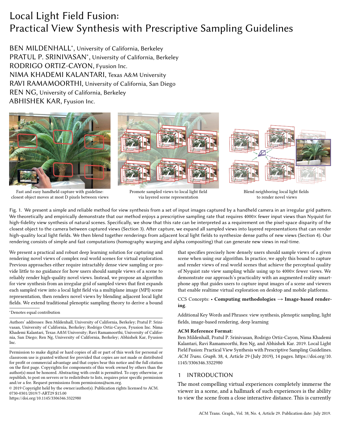
The approach introduces a two-stage pipeline. First, a deep three-dimensional convolutional neural network expands each captured image into a layered scene representation known as a multiplane image, which models local light fields and transparencies across depth planes. Second, novel viewpoints are rendered continuously in real time by projecting and blending adjacent multiplane representations using accumulated opacity to resolve occlusions. To support real-world use, the authors also developed an augmented reality smartphone capture application and evaluated performance across synthetic benchmarks and over 60 real handheld captures.

The primary finding is that this framework reduces the required number of captured views by up to 4000 times compared to traditional light field sampling standards while matching full perceptual visual quality. The maximum allowable disparity between adjacent views was determined to be 64 pixels, establishing a practical rule that governs the relationship between capture spacing, scene depth, and camera field of view. Quantitative and perceptual metrics demonstrated that the method consistently outperformed existing global mesh reconstruction, heuristic volume blending, and per-view deep warping techniques, particularly when handling fine geometric structures and non-Lambertian reflections.

These findings indicate that high-fidelity, interactive virtual exploration can be achieved casually using commodity handheld devices without specialized camera rigs or multi-hour reconstruction pipelines. By providing exact capture rules, the method eliminates costly guesswork and trial-and-error capture failures. Furthermore, the light rendering compute requirements make real-time interaction feasible on both desktop and mobile platforms.

Organizations developing virtual reality, augmented reality, or interactive 3D media applications should adopt the prescriptive sampling formulas to configure automated capture interfaces. Practitioners should ensure capture workflows guide users so that pixel shifts between adjacent views remain within the 64-pixel threshold. Future engineering work should explore multiresolution neural architectures to better support ultra-high-resolution imagery and improve geometric disambiguation in scenes with highly repetitive textures or moving objects.

The findings are supported by theoretical proofs, extensive quantitative evaluations, and diverse real-world demonstrations. However, users should exercise caution in environments containing subject motion or highly repetitive, untextured patterns, where local depth ambiguities can still produce minor visual artifacts.

Fyusion Inc.Texas A&M University University of California Berkeley University of California, San Diego augmented reality deep learning mobile platform Local Light Field Fusion Light Field Reconstruction Image-Based Rendering

arXiv: 1905.00889

Paper: Light field rendering, Marc Levoy et al. (1996). Introduces 4D light field rendering and sampling foundations that Local Light Field Fusion directly adapts and extends with multiplane image representations and sampling bounds.
Paper: The lumigraph, Steven J. Gortler et al. (1996). Provides the foundational plenoptic representation and geometry-assisted light field blending principles that motivate irregular-grid local light field fusion.
Paper: Layered depth images, Jonathan Shade et al. (1998). Pioneers layered depth representations for occlusion handling and novel view synthesis that serve as direct conceptual precursors to multiplane images.
Paper: High-quality video view interpolation using a layered representation, C. Lawrence Zitnick et al. (2004). Establishes layered scene decompositions for view interpolation to eliminate boundary and disocclusion artifacts.
Paper: MVSNet: Depth Inference for Unstructured Multi-view Stereo, Yao Yao et al. (2018). Demonstrates plane-sweep cost volumes for multi-view depth inference, underpinning modern deep learning pipelines for multiplane representations.

Paper: NeRF: Representing Scenes as Neural Radiance Fields for View Synthesis, Ben Mildenhall et al. (2020). Extends continuous view synthesis beyond local multiplane image blending by encoding 5D radiance fields into implicit coordinate neural networks (NeRF).
Paper: Mip-NeRF: A Multiscale Representation for Anti-Aliasing Neural Radiance Fields, Jonathan T. Barron et al. (2021). Improves neural radiance fields with cone tracing to resolve scale and anti-aliasing issues inherent in discrete view sampling.
Paper: Mip-NeRF 360: Unbounded Anti-Aliased Neural Radiance Fields, Jonathan T. Barron et al. (2022). Generalizes neural view synthesis from forward-facing captures to unbounded 360-degree scenes using scene contraction and proposal sampling.
Paper: Ref-NeRF: Structured View-Dependent Appearance for Neural Radiance Fields, Dor Verbin et al. (2022). Explicitly addresses complex specular highlights and view-dependent appearance that challenge traditional multiplane and radiance field fusion.
Paper: 3D Gaussian Splatting for Real-Time Radiance Field Rendering, Bernhard Kerbl et al. (2023). Replaces ray-marched implicit fields and blended MPIs with fast-rendering 3D Gaussian primitives to deliver real-time novel view synthesis.
Paper: Plenoxels: Radiance Fields without Neural Networks, Alex Yu et al. (2022). Develops explicit sparse voxel grids with spherical harmonics, achieving fast radiance field reconstruction without heavy neural networks.
Paper: PlenOctrees for Real-time Rendering of Neural Radiance Fields, Alex Yu et al. (2021). Converts continuous radiance fields into octree-based data structures to enable real-time view rendering on standard hardware.
Paper: TensoRF: Tensorial Radiance Fields, Anpei Chen et al. (2022). Factorizes 4D scene radiance fields using low-rank tensor decompositions to accelerate reconstruction and reduce memory overhead.

Abstract

We present a practical and robust deep learning solution for capturing and rendering novel views of complex real world scenes for virtual exploration. Previous approaches either require intractably dense view sampling or provide little to no guidance for how users should sample views of a scene to reliably render high-quality novel views. Instead, we propose an algorithm for view synthesis from an irregular grid of sampled views that first expands each sampled view into a local light field via a multiplane image (MPI) scene representation, then renders novel views by blending adjacent local light fields. We extend traditional plenoptic sampling theory to derive a bound that specifies precisely how densely users should sample views of a given scene when using our algorithm. In practice, we apply this bound to capture and render views of real world scenes that achieve the perceptual quality of Nyquist rate view sampling while using up to 4000x fewer views. We demonstrate our approach's practicality with an augmented reality smartphone app that guides users to capture input images of a scene and viewers that enable realtime virtual exploration on desktop and mobile platforms.

1 Introduction
2 Related Work
2.1 Plenoptic Sampling and Reconstruction
2.2 Geometry-Based View Synthesis
2.3 Deep Learning for View Synthesis
3 Theoretical Sampling Analysis
3.1 Nyquist Rate View Sampling
3.2 MPI Scene Representation and Rendering
3.3 View Sampling Rate Reduction
3.4 Image Space Interpretation of View Sampling
4 Practical View Synthesis Pipeline
4.1 MPI Prediction for Local Light Field Expansion
4.2 Continuous View Reconstruction by Blending
5 Training Our View Synthesis Pipeline
5.1 Training Dataset
5.2 Training Procedure
6 Experimental Evaluation
6.1 Sampling Theory Validation
6.2 Comparisons to Baseline Methods
6.3 Ablation Studies
7 Practical Usage
7.1 Prescriptive Scene Sampling Guidelines
7.2 Asymptotic Rendering Time and Space Complexity
7.3 Smartphone Capture App
7.4 Preprocessing
7.5 Real-Time Viewers
7.6 Limitations
8 Conclusion
A Baseline Methods Implementation Details
B Network Architecture
References

Knowls

Knowl 1 — Plenoptic Sampling Bound with Occlusion for Multiplane Image Representations
theoretical result
For a scene with closest depth $z_{\min}$ and farthest depth $z_{\max}$ , captured by a camera with focal length $f$ , pixel size $\Delta x$ , image width $W$ pixels, and maximum spatial frequency $K_x = \min(B_x, 1/(2\Delta x))$ (where $B_x$ is the highest continuous spatial frequency), predicting a multiplane image (MPI) with $D$ disparity-sampled depth layers and opacities reduces the required camera sampling rate. Under back-to-front alpha compositing—which convolves the light field spectrum with layer opacities—and ensuring that every scene point falls within the field of view of at least two adjacent views, the maximum camera baseline $\Delta u$ between neighboring views must satisfy:

$\Delta u \le \min \left( \frac{D}{2 K_x f (1/z_{\min} - 1/z_{\max})}, \frac{W \Delta x z_{\min}}{2 f} \right)$

For 2D viewpoint sampling lattices, this allows a reduction in the number of required view samples by up to $D^2$ relative to standard Nyquist view sampling ( $D=1$ ).
Knowl 2 — Disparity-Based View Sampling Bound
theoretical result
Assuming scene content extends to infinite distance ( $z_{\max} = \infty$ ) and spatial frequencies reach the Nyquist limit of the image sensor ( $K_x = 1/(2\Delta x)$ ), the camera baseline sampling bound translates directly into an upper bound on the maximum pixel disparity $d_{\max}$ of the closest scene point between adjacent input views:

$d_{\max} = \frac{\Delta u f}{\Delta x z_{\min}} \le \min\left(D, \frac{W}{2}\right)$

where $\Delta u$ is the camera baseline, $f$ is focal length, $\Delta x$ is pixel size, $z_{\min}$ is the closest depth, $W$ is the image width in pixels, and $D$ is the number of depth planes in each multiplane image (MPI). When $D=1$ , this bound recovers the classical Nyquist rate of at most $1$ pixel of disparity between adjacent views.
Knowl 3 — Prescriptive View Sampling Formula for Bounded Camera Trajectories
equation
For a camera with horizontal field of view $\theta$ used to sample $N$ images on a uniform 2D grid of side length $S$ (baseline $\Delta u = S/\sqrt{N}$ ), novel views can be reliably rendered across the bounding plane at Nyquist-level perceptual quality (subject to an empirical maximum disparity bound of $d_{\max} \le 64$ pixels) if the rendering resolution $W$ (pixels) and number of images $N$ satisfy:

$\frac{W}{\sqrt{N}} \le \frac{128 z_{\min} \tan(\theta/2)}{S}$

where $z_{\min}$ is the distance from the camera plane to the closest object in the scene. For a mobile phone camera with a $64^\circ$ field of view, this simplifies to:

$\frac{W}{\sqrt{N}} \le \frac{80 z_{\min}}{S}$
Knowl 4 — Alpha-Weighted Blending of Multiplane Image Renderings
model/method
To render a novel view at camera pose $p_t$ , multiple nearby predicted multiplane images (MPIs) $\{M_k\}$ at camera poses $\{p_k\}$ are each homography-warped and alpha-composited back-to-front into the target camera pose $p_t$ . This produces a set of RGB renderings $C_{t,k}$ and accumulated alpha maps $\alpha_{t,k}$ . The final color $C_t$ is synthesized via an alpha-weighted combination:

$C_t = \frac{\sum_k w_{t,k} \alpha_{t,k} C_{t,k}}{\sum_k w_{t,k} \alpha_{t,k}}$

where $w_{t,k}$ are viewpoint blending weights. For regularly spaced grids, bilinear weights from the 4 nearest MPIs are used. For irregular captures, weights over the 5 nearest MPIs are computed as:

$w_{t,k} \propto \exp\left(-\gamma \ell(p_t, p_k)\right), \quad \text{with } \gamma = \frac{f}{D z_{\min}}$

where $\ell(p_t, p_k)$ is the Euclidean distance between camera translation centers, $f$ is focal length, $z_{\min}$ is minimum scene depth, and $D$ is the number of planes. Weighting by accumulated alpha $\alpha_{t,k}$ ensures that disoccluded regions or areas outside a particular MPI's frustum are smoothly filled by other visible MPIs without ghosting or stretching artifacts.
Knowl 5 — 3D CNN Multiplane Image Prediction Pipeline
model/method
Local light field expansion converts each input image into a multiplane image (MPI) consisting of $D$ fronto-parallel RGB $\alpha$ planes sampled linearly in disparity within the reference view frustum. The prediction takes 5 input images: the reference view and its 4 nearest spatial neighbors. Each image is reprojected to the $D$ disparity planes to construct 5 plane sweep volumes (PSVs) of size $H \times W \times D \times 3$ .

A fully 3D convolutional neural network takes the 5 PSVs concatenated along the channel dimension ( $H \times W \times D \times 15$ ) and predicts 6 channels per voxel:
1. An opacity value $\alpha(x,y,d) \in [0, 1]$ generated via a sigmoid activation on one channel.
2. Five color selection weights $(s_1, \dots, s_5)$ generated by applying a softmax over the remaining four output channels and an explicit constant zero-logit channel, ensuring $\sum_{i=1}^5 s_i = 1$ .
The RGB color of voxel $(x, y, d)$ in the predicted MPI is formed by the linear combination $\text{RGB}(x,y,d) = \sum_{i=1}^5 s_i(x,y,d) \, \text{PSV}_i(x,y,d)$ . The 3D convolutional architecture enables the model to dynamically operate over a variable number of depth planes $D$ at test time.
Knowl 6 — End-to-End Training of MPI Prediction with Blending Supervision
model/method
The MPI prediction network is trained end-to-end through a differentiable multi-MPI rendering and blending pipeline. In each training step, two sets of 5 input views each are used to predict two separate MPIs. A held-out target view is rendered from both predicted MPIs and fused via alpha-weighted blending. The loss function is a VGG perceptual loss computed between the final blended image and the ground-truth target image.

Because warping, alpha compositing, and multi-MPI blending are differentiable, supervising only the final blended output teaches the network to set $\alpha \approx 0$ (creating alpha holes) in uncertain or occluded regions of an MPI, delegating the synthesis of those regions to neighboring MPIs.

Training proceeds in three stages:
1. Single MPI training for 500k iterations.
2. Two-MPI blended training for 100k iterations on synthetic data (SUNCG at $320 \times 240$ with up to $D=128$ , UnrealCV at $640 \times 480$ with up to $D=32$ ).
3. Real-data fine-tuning for 10k iterations on 24 real cellphone scenes with poses from structure-from-motion.
Optimization uses Adam with learning rate $2 \times 10^{-4}$ and batch size 1 across two GPUs.
Knowl 7 — 3D U-Net Architecture for Multiplane Image Prediction
model/method
The 3D CNN predicts an MPI from 5 concatenated Plane Sweep Volumes (15 input channels). All 3D convolutions use kernel size $3 \times 3 \times 3$ . Every intermediate convolution is followed by Layer Normalization and a ReLU activation. The layer configuration consists of:
- conv1_1: $15 \to 8$ chns, stride 1, dilation 1
- conv1_2: $8 \to 16$ chns, stride 2, dilation 1
- conv2_1: $16 \to 16$ chns, stride 1, dilation 1
- conv2_2: $16 \to 32$ chns, stride 2, dilation 1
- conv3_1: $32 \to 32$ chns, stride 1, dilation 1
- conv3_2: $32 \to 32$ chns, stride 1, dilation 1
- conv3_3: $32 \to 64$ chns, stride 2, dilation 1
- conv4_1, conv4_2, conv4_3: $64 \to 64$ chns, stride 1, dilation 2
- nnup5: $2\times$ nearest-neighbor upsampling on conv4_3 concatenated with conv3_3 ( $128$ chns)
- conv5_1: $128 \to 32$ chns, stride 1, dilation 1
- conv5_2, conv5_3: $32 \to 32$ chns, stride 1, dilation 1
- nnup6: $2\times$ upsampling on conv5_3 concatenated with conv2_2 ( $64$ chns)
- conv6_1: $64 \to 16$ chns, stride 1, dilation 1
- conv6_2: $16 \to 16$ chns, stride 1, dilation 1
- nnup7: $2\times$ upsampling on conv6_2 concatenated with conv1_2 ( $32$ chns)
- conv7_1: $32 \to 8$ chns, stride 1, dilation 1
- conv7_2: $8 \to 8$ chns, stride 1, dilation 1
- conv7_3: $8 \to 6$ chns, stride 1, dilation 1 (no normalization or activation; 1 channel feeds sigmoid for $\alpha$ , 4 channels feed softmax with a constant zero logit for 5 color selection weights).
Knowl 8 — Asymptotic Time and Storage Complexity of Local Light Field Fusion
theoretical result
When multiplane image plane count matches the maximum inter-view disparity ( $D = d_{\max} = \frac{W S}{2 \sqrt{N} z_{\min} \tan(\theta/2)}$ ) to satisfy the sampling bound for $N$ sampled views covering a baseline region of side length $S$ at image width $W$ :
1. Rendering Time per MPI: The number of voxels processed per MPI is $W^2 D$ , giving an asymptotic rendering time of: $W^2 D = \frac{W^3 S}{2 \sqrt{N} z_{\min} \tan(\theta/2)} = O(W^3 N^{-1/2})$ Rendering time per MPI decreases as more views $N$ are sampled, since fewer depth planes $D$ are required per MPI.
2. Total Storage Space: The storage requirement across all $N$ predicted MPIs scales as: $W^2 D \cdot N = \frac{W^3 S \sqrt{N}}{2 z_{\min} \tan(\theta/2)} = O(W^3 N^{1/2})$
3. Capture Time: Capturing $N$ images scales as $O(N)$ .

Knowl 9 — Quantitative View Synthesis Performance Across Disparity Sampling Rates

data/table

Evaluation on a synthetic benchmark of 8 UnrealCV scenes at $640 \times 480$ resolution across maximum adjacent-view disparities $d_{\max} \in \{16, 32, 64, 128\}$ pixels compares Local Light Field Fusion (LLFF) against Light Field Interpolation (LFI), Unstructured Lumigraph Rendering (ULR), Soft3D, and Backwards Warping Deep network (BW Deep), along with ablations (Single MPI and Average MPIs without alpha weighting):

	$d_{\max} = 16$			$d_{\max} = 32$			$d_{\max} = 64$			$d_{\max} = 128$
Algorithm	PSNR $\uparrow$	SSIM $\uparrow$	LPIPS $\downarrow$	PSNR $\uparrow$	SSIM $\uparrow$	LPIPS $\downarrow$	PSNR $\uparrow$	SSIM $\uparrow$	LPIPS $\downarrow$	PSNR $\uparrow$	SSIM $\uparrow$	LPIPS $\downarrow$
LFI	26.21	0.7776	0.2541	23.35	0.6982	0.3198	20.60	0.6243	0.3971	18.32	0.5560	0.4665
ULR	28.17	0.8320	0.1510	26.43	0.7987	0.1820	24.34	0.7679	0.2311	21.24	0.7062	0.3215
Soft3D	34.48	0.9430	0.1345	32.33	0.9216	0.1795	27.97	0.8588	0.2652	23.11	0.7382	0.3979
BW Deep	34.18	0.9433	0.1074	34.00	0.9476	0.1128	31.88	0.9192	0.1573	27.59	0.8363	0.2591
Single MPI	31.11	0.9482	0.1007	29.38	0.9424	0.1111	26.88	0.9250	0.1363	24.20	0.8734	0.1980
Avg. MPIs	32.67	0.9560	0.1140	31.34	0.9532	0.1248	29.31	0.9400	0.1423	27.02	0.8999	0.1961
Ours	34.57	0.9568	0.0942	34.48	0.9569	0.0954	33.58	0.9530	0.1012	31.96	0.9323	0.1374

LLFF achieves the highest PSNR and SSIM and lowest LPIPS at every sampling density. As disparity increases from $16$ to $128$ pixels, Soft3D and BW Deep degrade sharply due to stereo aggregation failure and disocclusion artifacts, whereas LLFF degrades significantly more gracefully.

Knowl 10 — Empirical Validation of the Nyquist Rate Sampling Bound
empirical result
Empirical evaluation of novel view synthesis quality across varying plane counts $D \in \{8, 16, 32, 64, 128\}$ and input view disparities $d_{\max} \in [1, 256]$ reveals:
1. Nyquist Quality at $4000\times$ Sparsity: Local Light Field Fusion matches the perceptual quality (LPIPS metric) of Nyquist-rate Light Field Interpolation ( $d_{\max} = 1$ ) up to an undersampling rate of $d_{\max} = 64$ pixels, provided $D \ge d_{\max}$ . In a 2D camera sampling grid, this represents an empirical reduction of $64^2 \approx 4000\times$ in required input images.
2. Plane Count Saturation: When $D \ge d_{\max}$ , adding more depth planes yields no further reduction in LPIPS error (for example, at $d_{\max}=32$ , error decreases from $D=8$ to $16$ to $32$ , but remains flat from $D=32$ to $128$ ), verifying that $D = d_{\max}$ planes is sufficient.
3. Occlusion Breakdown at Extreme Baselines: At $d_{\max} = 128$ , performance fails to reach Nyquist quality regardless of $D$ , because severe occlusions reduce the number of views observing background points, degrading stereo geometry estimation.
Knowl 11 — Limitations in Repetitive Textures, Scene Motion, and Resolution Scaling
limitation
Local Light Field Fusion exhibits three primary limitations:
1. Texture Ambiguity and Scene Motion: In regions with repetitive textures, uniform color, or moving scene elements between captures, the 3D CNN can assign high opacity to incorrect depth layers, producing floating or blurred artifacts in synthesized paths.
2. Cubic Scaling with Resolution: Memory footprint and per-MPI rendering complexity scale as $O(W^3 N^{-1/2})$ and total storage as $O(W^3 N^{1/2})$ with image width $W$ , making scaling to high-resolution images computationally demanding in GPU memory and compute.
3. Pose Estimation Dependence: The method relies on accurate offline structure-from-motion (such as COLMAP, taking 2–6 minutes for 20–30 views); real-time tracking from mobile AR frameworks (e.g., ARKit) produces poses that are not yet accurate enough to avoid rendering artifacts.

Coverage note — Omitted only the user interface details of the iOS ARKit capture app and specific OpenGL/Metal real-time viewer shader boilerplate, as these are direct software implementations of the core theoretical and algorithmic contributions.

References

1.Martín Abadi, Ashish Agarwal, Paul Barham, Eugene Brevdo, Zhifeng Chen, Craig Citro, Greg S. Corrado, Andy Davis, Jeffrey Dean, Matthieu Devin, et al. 2015. TensorFlow: Large-Scale Machine Learning on Heterogeneous Systems. (2015). https://www.tensorflow.org/
2.Robert Anderson, David Gallup, Jonathan T. Barron, Janne Kontkanen, Noah Snavely, Carlos Hernández, Sameer Agarwal, and Steven M Seitz. 2016. Jump: Virtual Reality Video. In SIGGRAPH Asia.
3.Chris Buehler, Michael Bosse, Leonard McMillan, Steven Gortler, and Michael Cohen. 2001. Unstructured Lumigraph Rendering. In SIGGRAPH.
4.Jin-Xiang Chai, Xin Tong, Sing-Chow Chan, and Heung-Yeung Shum. 2000. Plenoptic Sampling. In SIGGRAPH.
5.Gaurav Chaurasia, Sylvain Duchêne, Olga Sorkine-Hornung, and George Drettakis. 2013. Depth Synthesis and Local Warps for Plausible Image-based Navigation. In SIGGRAPH.
6.Qifeng Chen and Vladlen Koltun. 2017. Photographic Image Synthesis With Cascaded Refinement Networks. In ICCV.
7.Shenchang Eric Chen and Lance Williams. 1993. View Interpolation for Image Synthesis. In SIGGRAPH.
8.Abe Davis, Marc Levoy, and Fredo Durand. 2012. Unstructured Light Fields. In Computer Graphics Forum.
9.Paul Debevec, Camillo J. Taylor, and Jitendra Malik. 1996. Modeling and Rendering Architecture from Photographs: A Hybrid Geometry-and Image-Based Approach. In SIGGRAPH.
10.Piotr Didyk, Pitchaya Sitthi-Amorn, William T. Freeman, Fredo Durand, and Wojciech Matusik. 2013. 3DTV at Home: Eulerian-Lagrangian Stereo-to-Multiview Conversion. In SIGGRAPH Asia.
11.John Flynn, Ivan Neulander, James Philbin, and Noah Snavely. 2016. DeepStereo: Learning to Predict New Views From the World’s Imagery. In CVPR.
12.Steven J. Gortler, Radek Grzeszczuk, Richard Szeliski, and Michael F. Cohen. 1996. The Lumigraph. In SIGGRAPH.
13.Peter Hedman, Suhib Alsisan, Richard Szeliski, and Johannes Kopf. 2017. Casual 3D Photography. In SIGGRAPH Asia.
14.Peter Hedman and Johannes Kopf. 2018. Instant 3D Photography. In SIGGRAPH.
15.Peter Hedman, Julien Philip, True Price, Jan-Michael Frahm, George Drettakis, and Gabriel Brostow. 2018. Deep Blending for Free-Viewpoint Image-Based Rendering. In SIGGRAPH Asia.
16.Peter Hedman, Tobias Ritschel, George Drettakis, and Gabriel Brostow. 2016. Scalable Inside-Out Image-Based Rendering. In SIGGRAPH Asia.
17.Po-Han Huang, Kevin Matzen, Johannes Kopf, Narendra Ahuja, and Jia-Bin Huang. 2018. DeepMVS: Learning Multi-View Stereopsis. In CVPR.
18.Nima Khademi Kalantari, Ting-Chun Wang, and Ravi Ramamoorthi. 2016. Learning-Based View Synthesis for Light Field Cameras. In SIGGRAPH Asia.
19.Michael Kazhdan and Hugues Hoppe. 2013. Screened Poisson Surface Reconstruction. In SIGGRAPH.
20.Petr Kellnhofer, Piotr Didyk, Szu-Po Wang, Pitchaya Sitthi-Amorn, William Freeman, Fredo Durand, and Wojciech Matusik. 2017. 3DTV at Home: Eulerian-Lagrangian Stereo-to-Multiview Conversion. In SIGGRAPH.
21.Alex Kendall, Hayk Martirosyan, Saumitro Dasgupta, Peter Henry, Ryan Kennedy, Abraham Bachrach, and Adam Bry. 2017. End-to-End Learning of Geometry and Context for Deep Stereo Regression. In ICCV.
22.Diederik P. Kingma and Jimmy Ba. 2015. Adam: A Method for Stochastic Optimization. In ICLR.
23.Johannes Kopf, Fabian Langguth, Daniel Scharstein, Richard Szeliski, and Michael Goesele. 2013. Image-Based Rendering in the Gradient Domain. In SIGGRAPH Asia.
24.Philippe Lacroute and Marc Levoy. 1994. Fast Volume Rendering Using a Shear-Warp Factorization of the Viewing Transformation. In SIGGRAPH.
25.Douglas Lanman, Ramesh Raskar, Amit Agrawal, and Gabriel Taubin. 2008. Shield Fields: Modeling and Capturing 3D Occluders. In SIGGRAPH Asia.
26.Jimmy Lei Ba, Jamie Ryan Kiros, and Geoffrey E. Hinton. 2016. Layer Normalization. In arXiv:1607.06450.
27.Marc Levoy and Pat Hanrahan. 1996. Light Field Rendering. In SIGGRAPH.
28.Leonard McMillan and Gary Bishop. 1995. Plenoptic Modeling: An Image-Based Rendering System. In SIGGRAPH.
29.Rodrigo Ortiz-Cayon, Abdelaziz Djelouah, and George Drettakis. 2015. A Bayesian Approach for Selective Image-Based Rendering using Superpixels. In International Conference on 3D Vision (3DV).
30.Ryan S. Overbeck, Daniel Erickson, Daniel Evangelakos, Matt Pharr, and Paul Debevec. 2018. A System for Acquiring, Processing, and Rendering Panoramic Light Field Stills for Virtual Reality. In SIGGRAPH Asia.
31.Eric Penner and Li Zhang. 2017. Soft 3D Reconstruction for View Synthesis. In SIGGRAPH Asia.
32.Thomas Porter and Tom Duff. 1984. Compositing Digital Images. In SIGGRAPH.
33.Weichao Qiu, Fangwei Zhong, Yi Zhang, Siyuan Qiao, Zihao Xiao, Tae Soo Kim, Yizhou Wang, and Alan Yuille. 2017. UnrealCV: Virtual Worlds for Computer Vision. In ACM Multimedia Open Source Software Competition.
34.Johannes Lutz Schönberger and Jan-Michael Frahm. 2016. Structure-from-Motion Revisited. In CVPR.
35.Johannes Lutz Schönberger, Enliang Zheng, Marc Pollefeys, and Jan-Michael Frahm. 2016. Pixelwise View Selection for Unstructured Multi-View Stereo. In ECCV.
36.Jonathan Shade, Steven J. Gortler, Li wei He, and Richard Szeliski. 1998. Layered depth images. In SIGGRAPH.
37.Heung-Yeung Shum and Sing Bing Kang. 2000. A Review of Image-Based Rendering Techniques. In Proceedings of Visual Communications and Image Processing.
38.Sudipta Sinha, Johannes Kopf, Michael Goesele, Daniel Scharstein, and Richard Szeliski. 2012. Image-Based Rendering for Scenes with Reflections. In SIGGRAPH.
39.Shuran Song, Fisher Yu, Andy Zeng, Angel X Chang, Manolis Savva, and Thomas Funkhouser. 2017. Semantic Scene Completion from a Single Depth Image. In CVPR.
40.Pratul P. Srinivasan, Tongzhou Wang, Ashwin Sreelal, Ravi Ramamoorthi, and Ren Ng. 2017. Learning to Synthesize a 4D RGBD Light Field from a Single Image. In ICCV.
41.Rahul Swaminathan, Sing Bing Kang, Richard Szeliski, Antonio Criminisi, and Shree K. Nayar. 2002. On the Motion and Appearance of Specularities in Image Sequences. In ECCV.
42.Gordon Wetzstein, Douglas Lanman, Wolfgang Heidrich, and Ramesh Raskar. 2011. Layered 3D: Tomographic Image Synthesis for Attenuation-based Light Field and High Dynamic Range Displays. In SIGGRAPH.
43.Gordon Wetzstein, Douglas Lanman, Matthew Hirsch, and Ramesh Raskar. 2012. Tensor Displays: Compressive Light Field Synthesis using Multilayer Displays with Directional Backlighting. In SIGGRAPH.
44.Bennett Wilburn, Neel Joshi, Vaibhav Vaish, Eino-Ville Talvala, Emilio Antunez, Adam Barth, Andrew Adams, Marc Levoy, and Mark Horowitz. 2005. High Performance Imaging Using Large Camera Arrays. In SIGGRAPH.
45.Daniel N. Wood, Daniel I. Azuma, Ken Aldinger, Brian Curless, Tom Duchamp, David H. Salesin, and Werner Stuetzle. 2000. Surface Light Fields for 3D Photography. In SIGGRAPH.
46.Gaochang Wu, Mandan Zhao, Liangyong Wang, Qionghai Dai, Tianyou Chai, and Yebin Liu. 2017. Light Field Reconstruction Using Deep Convolutional Network on EPI. In CVPR.
47.Henry Wing Fung Yeung, Junhui Hou, Jie Chen, Yuk Ying Chung, and Xiaoming Chen. 2018. Fast Light Field Reconstruction with Deep Coarse-to-Fine Modeling of Spatial-Angular Clues. In ECCV.
48.Cha Zhang and Tsuhan Chen. 2003. Spectral Analysis for Sampling Image-Based Rendering Data. In IEEE Transactions on Circuits and Systems for Video Technology.
49.Richard Zhang, Phillip Isola, Alexei A Efros, Eli Shechtman, and Oliver Wang. 2018. The Unreasonable Effectiveness of Deep Features as a Perceptual Metric. In CVPR.
50.Zhoutong Zhang, Yebin Liu, and Qionghai Dai. 2015. Light Field from Micro-Baseline Image Pair. In CVPR.
51.Tinghui Zhou, Richard Tucker, John Flynn, Graham Fyffe, and Noah Snavely. 2018. Stereo Magnification: Learning View Synthesis using Multiplane Images. In SIGGRAPH.

Citation

MLA

Mildenhall, B., et al. “Local Light Field Fusion: Practical View Synthesis with Prescriptive Sampling Guidelines”. arXiv, 2019, http://arxiv.org/abs/1905.00889v1.

APA

Mildenhall, B., Srinivasan, P. P., Ortiz-Cayon, R., Kalantari, N. K., Ramamoorthi, R., Ng, R., & Kar, A. (2019). Local Light Field Fusion: Practical View Synthesis with Prescriptive Sampling Guidelines. arXiv. http://arxiv.org/abs/1905.00889v1

Chicago

Mildenhall, B., P. P. Srinivasan, R. Ortiz-Cayon, et al. 2019. “Local Light Field Fusion: Practical View Synthesis with Prescriptive Sampling Guidelines”. arXiv. http://arxiv.org/abs/1905.00889v1.

Harvard

Mildenhall, B. et al. (2019) “Local Light Field Fusion: Practical View Synthesis with Prescriptive Sampling Guidelines”, arXiv [Preprint]. Available at: http://arxiv.org/abs/1905.00889v1.

Vancouver

1. Mildenhall B, Srinivasan PP, Ortiz-Cayon R, Kalantari NK, Ramamoorthi R, Ng R, Kar A (2019) Local Light Field Fusion: Practical View Synthesis with Prescriptive Sampling Guidelines. arXiv

BibTeX

@article{mildenhall2019local,
  title = {Local Light Field Fusion: Practical View Synthesis with Prescriptive Sampling Guidelines},
  author = {Mildenhall, Ben and Srinivasan, Pratul P. and Ortiz-Cayon, Rodrigo and Kalantari, Nima Khademi and Ramamoorthi, Ravi and Ng, Ren and Kar, Abhishek},
  year = {2019},
  journal = {arXiv},
  url = {http://arxiv.org/abs/1905.00889v1},
  eprint = {1905.00889}
}

Metadata:arXiv

Access the Paper

This paper is available from its original source. Click below to access the PDF.

Open PDF

Local light field fusion

Abstract

Topics

Keywords

Table of Contents

Knowls

Knowl 1 — Plenoptic Sampling Bound with Occlusion for Multiplane Image Representations

Knowl 2 — Disparity-Based View Sampling Bound

Knowl 3 — Prescriptive View Sampling Formula for Bounded Camera Trajectories

Knowl 4 — Alpha-Weighted Blending of Multiplane Image Renderings

Knowl 5 — 3D CNN Multiplane Image Prediction Pipeline

Knowl 6 — End-to-End Training of MPI Prediction with Blending Supervision

Knowl 7 — 3D U-Net Architecture for Multiplane Image Prediction

Knowl 8 — Asymptotic Time and Storage Complexity of Local Light Field Fusion

Knowl 9 — Quantitative View Synthesis Performance Across Disparity Sampling Rates

Knowl 10 — Empirical Validation of the Nyquist Rate Sampling Bound

Knowl 11 — Limitations in Repetitive Textures, Scene Motion, and Resolution Scaling

References

Citation

BibTeX

Access the Paper