PlenOctrees for Real-time Rendering of Neural Radiance Fields

Alex YuRuilong LiMatthew TancikHao LiRen NgAngjoo Kanazawa

article2021ICCV1,342 citations

Develops PlenOctrees, an octree-based representation that pre-tabulates neural radiance fields using spherical harmonics to achieve real-time rendering at over 150 frames per second while preserving view-dependent visual quality.

Listen

Generating photorealistic, view-dependent 3D scenes from images using neural radiance fields has gained significant interest, but standard neural radiance approaches suffer from extremely slow rendering speeds that prevent real-time interactive use. The article evaluates an alternative representation called PlenOctrees (an octree-based radiance field representation) and investigates how spherical basis function choices, optimization, and compression techniques enable real-time rendering while maintaining visual fidelity.

The authors conducted experimental evaluations across standard synthetic and real-world benchmark datasets (such as NeRF-synthetic and Tanks&Temples). They analyzed rendering speeds, reconstruction quality, and memory storage using different spherical basis formulations, including spherical harmonics and learnable spherical Gaussians. The workflow involves training a modified neural radiance field model with spherical harmonics, converting it directly into an octree representation, and fine-tuning the structure using derived analytic rendering derivatives.

The findings demonstrate substantial performance gains. Converted and fine-tuned PlenOctrees achieve real-time rendering speeds averaging 167.7 frames per second on synthetic data and 42.2 frames per second on real-world datasets, compared to standard neural radiance baselines that render at less than 0.1 frames per second. Visual reconstruction quality remains on par with or slightly exceeds existing baselines after fine-tuning. Additionally, ablations show that lower-order spherical harmonics provide competitive visual quality while drastically reducing storage footprints and increasing framerates up to 261.7 frames per second. Applying standard quantization and data compression reduces overall file sizes by 20 to 30 times, making web-based transmission feasible.

These results indicate that volumetric neural rendering can transition from offline computational pipelines into interactive, consumer-facing applications, such as web and virtual reality environments, without compromising visual fidelity. The initial neural network training remains computationally intensive, requiring roughly 50 hours per scene on a single high-end processor, but the subsequent octree conversion and fine-tuning requires only about 10 minutes. Practitioners seeking to deploy real-time 3D viewers should adopt lower-order spherical harmonics with compression pipelines to balance visual accuracy against memory constraints, while future efforts should focus on reducing the upfront training duration.

Pinscreen University of California Berkeley University of Southern California closed-form expression geometry neural networks Neural Radiance Fields PlenOctrees real-time rendering

arXiv: 2103.14024 sxyu/plenoctree

Paper: NeRF: Representing Scenes as Neural Radiance Fields for View Synthesis, Ben Mildenhall et al. (2020). It introduces the fundamental Neural Radiance Fields (NeRF) representation and volumetric rendering formulation that PlenOctrees explicitly accelerates and tabulates into an octree.
Paper: Neural Sparse Voxel Fields, Lingjie Liu et al. (2020). It pioneers neural sparse voxel fields for bounding implicit scene evaluations within voxels to speed up rendering, providing direct context for voxel- and octree-based radiance field acceleration.
Paper: OctNet: Learning Deep 3D Representations at High Resolutions, Gernot Riegler et al. (2016). It introduces deep 3D representations utilizing hierarchical octree data structures to overcome volumetric cubic complexity, establishing the data structuring principles used in PlenOctrees.
Paper: Scene Representation Networks: Continuous 3D-Structure-Aware Neural Scene Representations, V. Sitzmann et al. (2019). It lays foundational ground for coordinate-based neural representations and differentiable ray-marching for continuous 3D scene rendering from 2D images.
Paper: Light field rendering, Marc Levoy et al. (1996). It establishes classic light field sampling and view-dependent radiance interpolation without heavy geometry, inspiring explicit plenoptic tabulation techniques.

Paper: Plenoxels: Radiance Fields without Neural Networks, Alex Yu et al. (2022). It extends PlenOctrees' spherical-harmonic voxel concept by completely discarding neural networks and optimizing explicit sparse voxel grids directly from scratch.
Paper: Direct Voxel Grid Optimization: Super-fast Convergence for Radiance Fields Reconstruction, Cheng Sun et al. (2021). It builds directly upon real-time explicit grid optimization by developing direct voxel grid optimization with post-activated interpolation for rapid convergence.
Paper: TensoRF: Tensorial Radiance Fields, Anpei Chen et al. (2022). It generalizes explicit radiance field representations like PlenOctrees by factorizing 3D voxel grids into low-rank tensor components for compact memory and fast rendering.
Paper: Instant neural graphics primitives with a multiresolution hash encoding, Thomas Müller et al. (2022). It advances real-time neural radiance field rendering and training by replacing explicit tree structures with a multiresolution hash table encoding.
Paper: 3D Gaussian Splatting for Real-Time Radiance Field Rendering, Bernhard Kerbl et al. (2023). It represents a major evolution in real-time view-dependent rendering, moving from octree-based voxel grids to explicit 3D Gaussian primitives with spherical harmonics.
Paper: Ref-NeRF: Structured View-Dependent Appearance for Neural Radiance Fields, Dor Verbin et al. (2022). It refines the modeling of view-dependent appearances and specularities in radiance fields, addressing limitations inherent to standard spherical harmonic parameterizations.
Paper: 4D Gaussian Splatting for Real-Time Dynamic Scene Rendering, Guanjun Wu et al. (2023). It builds upon explicit real-time radiance field rendering techniques to extend high-framerate novel view synthesis to dynamic 4D scenes.

Cover for PlenOctrees for Real-time Rendering of Neural Radiance Fields

Abstract

We introduce a method to render Neural Radiance Fields (NeRFs) in real time using PlenOctrees, an octree-based 3D representation which supports view-dependent effects. Our method can render 800x800 images at more than 150 FPS, which is over 3000 times faster than conventional NeRFs. We do so without sacrificing quality while preserving the ability of NeRFs to perform free-viewpoint rendering of scenes with arbitrary geometry and view-dependent effects. Real-time performance is achieved by pre-tabulating the NeRF into a PlenOctree. In order to preserve view-dependent effects such as specularities, we factorize the appearance via closed-form spherical basis functions. Specifically, we show that it is possible to train NeRFs to predict a spherical harmonic representation of radiance, removing the viewing direction as an input to the neural network. Furthermore, we show that PlenOctrees can be directly optimized to further minimize the reconstruction loss, which leads to equal or better quality compared to competing methods. Moreover, this octree optimization step can be used to reduce the training time, as we no longer need to wait for the NeRF training to converge fully. Our real-time neural rendering approach may potentially enable new applications such as 6-DOF industrial and product visualizations, as well as next generation AR/VR systems. PlenOctrees are amenable to in-browser rendering as well; please visit the project page for the interactive online demo, as well as video and code: this https URL

Topics

closed-form expression geometry neural networks neural radiance fields optimization reconstruction view-dependent viewpoint optimization problems

Keywords

Neural Radiance Fields PlenOctrees real-time rendering spherical harmonics spherical Gaussians radiance transfer NeRF-synthetic dataset Neural Volumes

1 Introduction
2 Related Work
3 Preliminaries
3.1 Neural Radiance Fields
4 Method
4.1 NeRF-SH: NeRF with Spherical Harmonics
4.2 PlenOctree: Octree-based Radiance Fields
4.3 PlenOctree Optimization
5 Results
5.1 Experimental Setup
5.2 Quality Evaluation
5.3 Speed Trade-off Analysis
5.4 Indirect Acceleration of NeRF Training
5.5 Real-time and In-browser Applications
6 Discussion
References
A Additional Results
A.1 Detailed comparisons
A.2 Spherical Basis Function Ablation
B Technical Details
B.1 Spherical Basis Functions: SH and SG
B.2 PlenOctree Compression
B.3 Analytic Derivatives of PlenOctree Rendering
B.3.1 Definitions
B.3.2 Derivation of the Derivatives
B.4 NeRF-SH Training Details
B.5 PlenOctree Optimization Details

Knowls

Knowl 1 — Analytic Gradient of Volume Rendering with Respect to Segment Densities
theoretical result
In piecewise-constant volume rendering along a camera ray partitioned into $N$ segments with endpoints $\{t_i\}_{i=0}^N$ , segment lengths $\delta_i = t_{i+1} - t_i$ , constant densities $\sigma = (\sigma_0, \dots, \sigma_{N-1})$ where $\sigma_i \ge 0$ , segment colors $c = (c_0, \dots, c_{N-1}) \in [0, 1]^{N \times 3}$ , and background color $c_N \in [0, 1]^3$ , the accumulated transmittance from $t_0$ to $t_i$ is:

$T_i(\sigma) = \prod_{j=0}^{i-1} \exp(-\delta_j \sigma_j)$

with $T_0(\sigma) = 1$ . The segment rendering weights are defined as $w_i(\sigma) = T_i(\sigma)(1 - \exp(-\sigma_i \delta_i)) = T_i(\sigma) - T_{i+1}(\sigma)$ for $i \in \{0, \dots, N-1\}$ and $w_N(\sigma) = T_N(\sigma)$ . The composited ray color is:

$\hat{C}(\sigma, c) = T_N(\sigma) c_N + \sum_{i=0}^{N-1} T_i(\sigma)(1 - e^{-\sigma_i \delta_i}) c_i = \sum_{i=0}^N w_i(\sigma) c_i$

The analytic derivative of the rendered ray color $\hat{C}$ with respect to the segment density $\sigma_i$ is:

$\frac{\partial \hat{C}}{\partial \sigma_i}(\sigma, c) = \delta_i \left( c_i T_{i+1}(\sigma) - \sum_{k=i+1}^N c_k w_k(\sigma) \right)$

When segment density is parameterized through an unconstrained network output $\tilde{\sigma}_i \in \mathbb{R}$ via a rectifier $\sigma_i = \max(0, \tilde{\sigma}_i)$ , the gradient is set to $0$ whenever $\tilde{\sigma}_i \le 0$ . For multi-channel RGB colors, the derivative is summed across color channels.

In an octree volume renderer, this gradient can be evaluated in two rendering passes: the first pass accumulates the total weighted color $\sum_{k=0}^N c_k w_k(\sigma)$ , and the second pass marches along the ray while subtracting prefix terms to compute the suffix sum $\sum_{k=i+1}^N c_k w_k(\sigma)$ with $O(1)$ auxiliary memory.
Knowl 2 — Analytic Gradient of Volume Rendering with Respect to Segment Colors and Spherical Harmonics
theoretical result
Under the piecewise-constant volume rendering formulation along a ray divided into $N$ segments with segment lengths $\delta_i = t_{i+1} - t_i$ , densities $\sigma_i \ge 0$ , and segment colors $c_i \in [0, 1]^3$ , the rendered color $\hat{C}(\sigma, c) = \sum_{i=0}^N w_i(\sigma) c_i$ is a linear combination of segment colors weighted by:

$w_i(\sigma) = T_i(\sigma)(1 - \exp(-\sigma_i \delta_i)) = T_i(\sigma) - T_{i+1}(\sigma)$

where $T_i(\sigma) = \prod_{j=0}^{i-1} \exp(-\delta_j \sigma_j)$ is the accumulated transmittance and $w_N(\sigma) = T_N(\sigma)$ is the background weight.

The analytic derivative of the rendered color with respect to the color vector $c_i$ of segment $i$ is:

$\frac{\partial \hat{C}}{\partial c_i}(\sigma, c) = w_i(\sigma)$

When segment color is parameterized by spherical basis functions (such as Spherical Harmonics $Y_\ell^m$ with RGB coefficients $k_{\ell, i}^m \in \mathbb{R}^3$ evaluated at ray direction $d$ ), the basis values $Y_\ell^m(d)$ remain constant along the ray. By the chain rule, the derivative with respect to each basis coefficient $k_{\ell, i}^m$ is:

$\frac{\partial \hat{C}}{\partial k_{\ell, i}^m} = w_i(\sigma) Y_\ell^m(d)$
Knowl 3 — Two-Stage Compression Pipeline for Octree Radiance Fields
algorithm
To enable fast downloading and real-time execution of Octree Radiance Fields (ORFs) within web browsers, uncompressed tree files are compressed using a two-stage pipeline combining lossy vector quantization and lossless tree compression:
1. Median-Cut Vector Quantization: Voxel densities $\sigma$ are retained unquantized. For each Spherical Harmonics (SH) basis function component $(\ell, m)$ , the three-dimensional RGB coefficients $k_\ell^m \in \mathbb{R}^3$ of all active voxels are quantized into $2^{16}$ representative RGB centroids using the median-cut algorithm. For each SH component, a $2^{16} \times 3$ codebook is stored in float16 precision, and each octree leaf node stores a 16-bit integer (int16) index pointing to its entry in the codebook.
2. Lossless Tree Compression: The full octree topology, including tree pointers, densities, and codebook indices, is compressed using the standard DEFLATE algorithm (ZLIB).
Additionally, browser representations use 9 SH basis functions (degree $\ell_{\max} = 2$ ) instead of 16 or 25 and apply a looser bounding box to reduce occupied voxel count. This entire compression scheme reduces the raw ORF file size by a factor of $20\times$ to $30\times$ . The browser client decompresses the tree structure fully into memory before starting GPU rendering.
Knowl 4 — Mathematical Formulation of Spherical Harmonics and Spherical Gaussians for Radiance Fields
model/method
Directional view-dependent radiance $L(d)$ for unit viewing direction $d = (\theta, \phi) \in \mathbb{S}^2$ can be parameterized in volume voxels using either Spherical Harmonics (SH) or Spherical Gaussians (SG):
- Real Spherical Harmonics (SH): The complex SH basis of degree $\ell \in \mathbb{N} \cup \{0\}$ and order $m \in \{-\ell, \dots, \ell\}$ is defined as:
$Y_\ell^m(\theta, \phi) = \sqrt{\frac{2\ell + 1}{4\pi} \frac{(\ell - m)!}{(\ell + m)!}} P_\ell^m(\cos \theta) e^{i m \phi}$

where $P_\ell^m$ are associated Legendre polynomials. The real SH basis $Y_\ell^m: \mathbb{S}^2 \to \mathbb{R}$ is:

$Y_\ell^m(\theta, \phi) = \begin{cases} \sqrt{2}(-1)^m \operatorname{Im}[Y_\ell^{|m|}] & \text{if } m < 0 \\ Y_\ell^0 & \text{if } m = 0 \\ \sqrt{2}(-1)^m \operatorname{Re}[Y_\ell^m] & \text{if } m > 0 \end{cases}$

Radiance is expanded linearly as $L(d) = \sum_{\ell=0}^{\ell_{\max}} \sum_{m=-\ell}^\ell k_\ell^m Y_\ell^m(\theta, \phi)$ with RGB coefficient vectors $k_\ell^m \in \mathbb{R}^3$ .
- Spherical Gaussians (SG): A normalized SG lobe with lobe axis $p \in \mathbb{S}^2$ and sharpness/bandwidth $\lambda \in \mathbb{R}$ is defined as:
$G(d; p, \lambda) = e^{\lambda (d \cdot p - 1)}$

A spherical radiance signal is represented with $n$ learnable SG components:

$L(d) \approx \sum_{j=1}^n k_j G_j(d; p_j, \lambda_j)$

where $k_j \in \mathbb{R}^3$ are RGB lobe weights.
Knowl 5 — Training Protocol for NeRF-SH and Direct Optimization of PlenOctrees
experimental setup
The training and optimization pipeline for NeRF with Spherical Harmonics (NeRF-SH) and PlenOctrees (Octree Radiance Fields, ORF) operates in two successive stages:
1. NeRF-SH Training:
  - Implementation: Built on JaxNeRF.
  - Ray sampling: Batch size of $1024$ rays, sampling $64$ points in the coarse volume and $128$ additional points in the fine volume per ray.
  - Optimizer: Adam optimizer with learning rate starting at $5 \times 10^{-4}$ and decaying exponentially to $5 \times 10^{-6}$ .
  - Duration: Trained for $2 \times 10^6$ iterations (approximately $50$ hours on a single NVIDIA V100 GPU).
2. Direct PlenOctree Optimization (Fine-Tuning):
  - Optimizer: Stochastic Gradient Descent (SGD) updating voxel densities and basis coefficients directly on the training set.
  - Learning rate: Fixed learning rate of $1 \times 10^7$ for NeRF-synthetic and $1.5 \times 10^6$ for Tanks & Temples.
  - Epochs & Early Stopping: Maximum of $80$ epochs for synthetic scenes and $40$ epochs for Tanks & Temples, monitored via validation set PSNR (holding out 10% of training data for Tanks & Temples).
  - Computation precision: Optimized in float32, stored in float16 to reduce memory.
  - Runtime: Approximately $10$ minutes per scene on a single NVIDIA V100 GPU.

Knowl 6 — Comparative View Synthesis and Speed Metrics on NeRF-Synthetic Dataset

data/table

The table below compares novel view synthesis reconstruction quality (PSNR, SSIM, LPIPS) and rendering frame rate (FPS) on the NeRF-synthetic benchmark across baseline neural rendering architectures and Octree Radiance Fields:

Model	PSNR $\uparrow$	SSIM $\uparrow$	LPIPS $\downarrow$	FPS $\uparrow$
NeRF (original)	31.01	0.947	0.081	0.023
NeRF	31.69	0.953	0.068	0.045
SRN	22.26	0.846	0.170	0.909
Neural Volumes	26.05	0.893	0.160	3.330
NSVF	31.75	0.953	0.047	0.815
AutoInt (8 sections)	25.55	0.911	0.170	0.380
NeRF-SH	31.57	0.952	0.063	0.051
ORF from NeRF-SH	31.02	0.951	0.066	167.68
ORF after fine-tuning	31.71	0.958	0.053	167.68

Fine-tuned PlenOctrees match the rendering quality of continuous implicit representations (PSNR of $31.71$ dB vs. $31.75$ dB for NSVF and $31.69$ dB for NeRF) while rendering at $167.68$ FPS, achieving an acceleration of over $200\times$ compared to NSVF ( $0.815$ FPS) and over $3{,}700\times$ compared to NeRF ( $0.045$ FPS).

Knowl 7 — Per-Scene Quantitative Performance on Tanks & Temples Dataset

data/table

The table below provides the per-scene quantitative breakdown across five real scenes from the Tanks & Temples benchmark for PSNR, SSIM, LPIPS, and rendering speed (FPS):

Metric / Method	Barn	Caterpillar	Family	Ignatius	Truck	Mean
PSNR $\uparrow$
NeRF (original)	24.05	23.75	30.29	25.43	25.36	25.78
NeRF	27.39	25.24	32.47	27.95	26.66	27.94
SRN	22.44	21.14	27.57	26.70	22.62	24.09
Neural Volumes	20.82	20.71	28.72	26.54	21.71	23.70
NSVF	27.16	26.44	33.58	27.91	26.92	28.40
NeRF-SH	27.05	25.06	32.28	28.06	26.66	27.82
PlenOctree from NeRF-SH	25.78	24.80	32.04	27.92	26.15	27.34
PlenOctree after fine-tuning	26.80	25.29	32.85	28.19	26.83	27.99
SSIM $\uparrow$
NeRF (original)	0.750	0.860	0.932	0.920	0.860	0.864
NeRF	0.842	0.892	0.951	0.940	0.896	0.904
SRN	0.741	0.834	0.908	0.920	0.832	0.847
Neural Volumes	0.721	0.819	0.916	0.922	0.793	0.834
NSVF	0.823	0.900	0.954	0.930	0.895	0.900
NeRF-SH	0.838	0.891	0.949	0.940	0.895	0.902
PlenOctree from NeRF-SH	0.820	0.889	0.948	0.940	0.889	0.897
PlenOctree after fine-tuning	0.856	0.907	0.962	0.948	0.914	0.917
LPIPS $\downarrow$
NeRF (original)	0.395	0.196	0.098	0.111	0.192	0.198
NeRF	0.286	0.189	0.092	0.102	0.173	0.168
SRN	0.448	0.278	0.134	0.128	0.266	0.251
Neural Volumes	0.479	0.280	0.111	0.117	0.312	0.260
NSVF	0.307	0.141	0.063	0.106	0.148	0.153
NeRF-SH	0.291	0.185	0.091	0.091	0.175	0.167
PlenOctree from NeRF-SH	0.296	0.188	0.094	0.092	0.180	0.170
PlenOctree after fine-tuning	0.226	0.148	0.069	0.080	0.130	0.131
FPS $\uparrow$
NeRF (original)	0.007	0.007	0.007	0.007	0.007	0.007
NeRF	0.013	0.013	0.013	0.013	0.013	0.013
SRN	0.250	0.250	0.250	0.250	0.250	0.250
Neural Volumes	1.000	1.000	1.000	1.000	1.000	1.000
NSVF	10.74	5.415	2.625	6.062	5.886	6.146
NeRF-SH	0.015	0.015	0.015	0.015	0.015	0.015
PlenOctree (ours)	46.94	54.00	32.33	15.67	62.16	42.22

On real-world outward-facing scenes, fine-tuned PlenOctrees achieve the lowest mean perceptual error (LPIPS of $0.131$ vs. $0.153$ for NSVF and $0.168$ for NeRF) while rendering at an average speed of $42.22$ FPS (compared to $6.146$ FPS for NSVF and $0.013$ FPS for NeRF).

Knowl 8 — Ablation of PlenOctree Model Size, Frame Rate, and Reconstruction Quality

data/table

The table below presents quantitative ablation results across four PlenOctree configurations (Ours-1.9G, Ours-1.4G, Ours-0.4G, and Ours-0.3G) evaluated over eight scenes of the NeRF-synthetic dataset:

Configuration	Chair	Drums	Ficus	Hotdog	Lego	Materials	Mic	Ship	Mean
PSNR $\uparrow$
Ours-1.9G	34.66	25.31	30.79	36.79	32.95	29.76	33.97	29.42	31.71
Ours-1.4G	34.66	25.30	30.82	36.36	32.96	29.75	33.98	29.29	31.64
Ours-0.4G	32.92	24.82	30.07	36.06	31.61	28.89	32.19	29.04	30.70
Ours-0.3G	32.03	24.10	29.42	34.46	30.25	28.44	30.78	27.36	29.60
Size (GB) $\downarrow$
Ours-1.9G	0.830	1.240	1.791	2.674	2.067	3.682	0.442	2.689	1.93
Ours-1.4G	0.671	0.852	0.943	1.495	1.421	3.060	0.569	1.881	1.36
Ours-0.4G	0.176	0.350	0.287	0.419	0.499	0.295	0.327	1.195	0.44
Ours-0.3G	0.131	0.183	0.286	0.403	0.340	0.503	0.159	0.381	0.30
FPS $\uparrow$
Ours-1.9G	352.4	175.9	85.6	95.5	186.8	64.2	324.9	56.0	167.7
Ours-1.4G	399.7	222.2	147.3	163.5	247.9	68.0	393.8	75.4	214.7
Ours-0.4G	639.6	290.0	208.7	273.5	339.0	268.0	522.6	86.7	328.5
Ours-0.3G	767.6	424.1	203.8	271.7	443.6	189.1	796.4	181.1	409.7

These results establish the trade-off envelope: scaling down the average tree size by $6.4\times$ (from $1.93$ GB to $0.30$ GB) accelerates rendering speed by $2.44\times$ (from $167.7$ FPS to $409.7$ FPS) while incurring an average PSNR degradation of $2.11$ dB (from $31.71$ dB to $29.60$ dB).

Knowl 9 — Ablation of Spherical Harmonics Degree and Spherical Gaussians

data/table

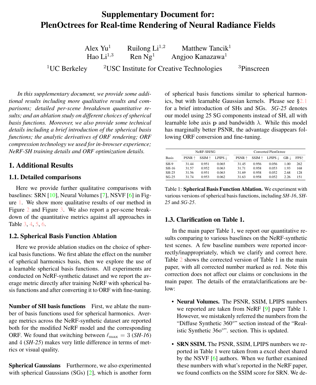
The table below details the performance comparison between varying numbers of Spherical Harmonics (SH) basis components (SH-9 with $\ell_{\max}=2$ , SH-16 with $\ell_{\max}=3$ , SH-25 with $\ell_{\max}=4$ ) and 25 learnable Spherical Gaussian components (SG-25), both in the neural stage (NeRF-SH/SG) and after PlenOctree conversion with fine-tuning:

	NeRF-SH/SG			Converted PlenOctree
Basis	PSNR $\uparrow$	SSIM $\uparrow$	LPIPS $\downarrow$	PSNR $\uparrow$	SSIM $\uparrow$	LPIPS $\downarrow$	GB $\downarrow$	FPS $\uparrow$
SH-9	31.44	0.951	0.065	31.45	0.956	0.056	1.00	262
SH-16	31.57	0.952	0.063	31.71	0.958	0.053	1.93	168
SH-25	31.56	0.951	0.063	31.69	0.958	0.052	2.68	128
SG-25	31.74	0.953	0.062	31.63	0.958	0.052	2.26	151

Increasing the SH basis from 16 to 25 functions yields negligible visual metric gains ( $31.71$ vs. $31.69$ dB PSNR, $0.053$ vs. $0.052$ LPIPS) while increasing storage requirements by $39\%$ ( $1.93$ GB to $2.68$ GB) and decreasing frame rate by $24\%$ ( $168$ FPS to $128$ FPS). While SG-25 yields marginally higher PSNR in the initial continuous neural field ( $31.74$ dB vs. $31.57$ dB), this advantage vanishes after octree extraction and fine-tuning, where SH-16 provides superior PSNR ( $31.71$ dB vs. $31.63$ dB), lower storage ( $1.93$ GB vs. $2.26$ GB), and faster rendering ( $168$ FPS vs. $151$ FPS).

Coverage note — Deliberately omitted qualitative comparison image figures (Figures 1, 2, 3) whose perceptual differences are captured quantitatively in the tables, and the per-scene full table for Table 3 since Table 2 and Table 6 convey the aggregated conclusions.

References

1.Boyang Deng, Jonathan T. Barron, and Pratul P. Srinivasan. JaxNeRF: an efficient JAX implementation of NeRF, 2020. 4
2.Ronald Aylmer Fisher. Dispersion on a sphere. Proceedings of the Royal Society of London. Series A. Mathematical and Physical Sciences, 217(1130):295–305, 1953. 1, 2
3.Paul Heckbert. Color image quantization for frame buffer display. SIGGRAPH, 1982. 3
4.Diederik P Kingma and Jimmy Ba. Adam: A method for stochastic optimization. In ICLR, 2015. 4
5.Zhengqin Li, Mohammad Shafiei, Ravi Ramamoorthi, Kalyan Sunkavalli, and Manmohan Chandraker. Inverse rendering for complex indoor scenes: Shape, spatially-varying lighting and svbrdf from a single image. In CVPR, pages 2475–2484, 2020. 2
6.Lingjie Liu, Jiatao Gu, Kyaw Zaw Lin, Tat-Seng Chua, and Christian Theobalt. Neural sparse voxel fields. NeurIPS, 2020. 1
7.Stephen Lombardi, Tomas Simon, Jason Saragih, Gabriel Schwartz, Andreas Lehrmann, and Yaser Sheikh. Neural volumes: Learning dynamic renderable volumes from images. ACM Transactions on Graphics (TOG), 38(4):65:1–65:14, 2019. 1
8.Jean loup Gailly and Mark Adler. zlib, 2017. 3
9.Ben Mildenhall, Pratul P. Srinivasan, Matthew Tancik, Jonathan T. Barron, Ravi Ramamoorthi, and Ren Ng. NeRF: Representing scenes as neural radiance fields for view synthesis. ECCV, 2020. 1
10.Vincent Sitzmann, Michael Zollhöfer, and Gordon Wetzstein. Scene representation networks: Continuous 3d-structure-aware neural scene representations. In NeurIPS, 2019. 1
11.Peter-Pike Sloan, Jan Kautz, and John Snyder. Precomputed radiance transfer for real-time rendering in dynamic, low-frequency lighting environments. In SIGGRAPH, pages 527–536, 2002. 2
12.Yu-Ting Tsai and Zen-Chung Shih. All-frequency precomputed radiance transfer using spherical radial basis functions and clustered tensor approximation. ACM Transactions on graphics (TOG), 25(3):967–976, 2006. 2

Citation

MLA

Yu, A., et al. “PlenOctrees for Real-time Rendering of Neural Radiance Fields”. arXiv, 2021, http://arxiv.org/abs/2103.14024v2.

APA

Yu, A., Li, R., Tancik, M., Li, H., Ng, R., & Kanazawa, A. (2021). PlenOctrees for Real-time Rendering of Neural Radiance Fields. arXiv. http://arxiv.org/abs/2103.14024v2

Chicago

Yu, A., R. Li, M. Tancik, H. Li, R. Ng, and A. Kanazawa. 2021. “PlenOctrees for Real-time Rendering of Neural Radiance Fields”. arXiv. http://arxiv.org/abs/2103.14024v2.

Harvard

Yu, A. et al. (2021) “PlenOctrees for Real-time Rendering of Neural Radiance Fields”, arXiv [Preprint]. Available at: http://arxiv.org/abs/2103.14024v2.

Vancouver

1. Yu A, Li R, Tancik M, Li H, Ng R, Kanazawa A (2021) PlenOctrees for Real-time Rendering of Neural Radiance Fields. arXiv

BibTeX

@article{yu2021plenoctrees,
  title = {PlenOctrees for Real-time Rendering of Neural Radiance Fields},
  author = {Yu, Alex and Li, Ruilong and Tancik, Matthew and Li, Hao and Ng, Ren and Kanazawa, Angjoo},
  year = {2021},
  journal = {arXiv},
  url = {http://arxiv.org/abs/2103.14024v2},
  eprint = {2103.14024}
}

Metadata:arXiv

Source Code

This paper has an official code repository available. Click below to access the source code.

View Repository

Access the Paper

This paper is available from its original source. Click below to access the PDF.

Open PDF

License: https://creativecommons.org/licenses/by/4.0/

PlenOctrees for Real-time Rendering of Neural Radiance Fields

Abstract

Topics

Keywords

Table of Contents

Knowls

Knowl 1 — Analytic Gradient of Volume Rendering with Respect to Segment Densities

Knowl 2 — Analytic Gradient of Volume Rendering with Respect to Segment Colors and Spherical Harmonics

Knowl 3 — Two-Stage Compression Pipeline for Octree Radiance Fields

Knowl 4 — Mathematical Formulation of Spherical Harmonics and Spherical Gaussians for Radiance Fields

Knowl 5 — Training Protocol for NeRF-SH and Direct Optimization of PlenOctrees

Knowl 6 — Comparative View Synthesis and Speed Metrics on NeRF-Synthetic Dataset

Knowl 7 — Per-Scene Quantitative Performance on Tanks & Temples Dataset

Knowl 8 — Ablation of PlenOctree Model Size, Frame Rate, and Reconstruction Quality

Knowl 9 — Ablation of Spherical Harmonics Degree and Spherical Gaussians

References

Citation

BibTeX

Source Code

Access the Paper