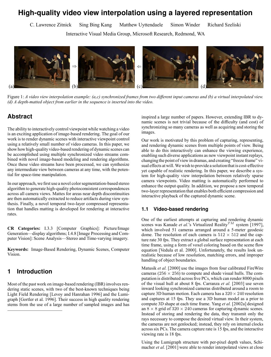
High-quality video view interpolation using a layered representation

C. Lawrence ZitnickS. KangM. UyttendaeleSimon A. J. WinderR. Szeliski

article2004TOG1,664 citations

Presents a novel two-layer depth and matting representation with a segmentation-based stereo algorithm that enables real-time, interactive free-viewpoint video synthesis from a sparse set of synchronized cameras.

Listen

Capturing dynamic, real-world scenes and allowing viewers to interactively change their viewpoint—creating continuous freeze-frame or slow-motion effects—traditionally demands either expensive, dense camera arrays or extensive manual post-production. Existing view-interpolation systems often suffer from poor visual quality, slow processing speeds, or severe visual artifacts around object boundaries. To solve this, the article evaluates and demonstrates a complete system capable of high-quality, interactive video view interpolation using a relatively sparse set of synchronized video cameras.

The system relies on an offline processing pipeline paired with a real-time graphics processor unit renderer. The researchers deployed an eight-camera synchronized array recording 1024 by 768 resolution video at 15 frames per second along a 30-degree arc. The methodology applies a color-segmentation stereo algorithm to recover accurate 3D scene geometry, extracts boundary matting to separate mixed foreground-background pixels near depth discontinuities, and compresses the scene into an efficient two-layer format using spatial and temporal predictions before rendering.

The findings establish that this layered approach significantly enhances visual fidelity and rendering efficiency. First, the two-layer representation isolates depth edges into a sparse boundary strip, eliminating jaggies and color bleeding artifacts without requiring complex global 3D models. Second, the custom hybrid compression scheme achieves high signal-to-noise ratios and decodes a frame in roughly nine milliseconds, enabling interactive playback. Third, the rendering system achieves real-time interactive performance, running at up to 20 to 30 frames per second depending on image resolution and memory caching. Fourth, the system exhibits substantial geometric robustness, tolerating up to 150 to 200 pixels of disparity and maintaining visual quality even when the spacing between cameras is tripled. Finally, the extracted geometry enables automated 3D special effects, such as seamless video object insertion, without manual rotoscoping.

These results demonstrate that media producers and application developers can deliver high-quality, free-viewpoint dynamic video experiences at substantially lower hardware and labor costs. The separation of heavy geometric computation into an offline stage enables lightweight, interactive playback on standard consumer personal computers. This makes the architecture particularly well-suited for instructional sports videos, dynamic event archiving, and interactive entertainment rather than live broadcasts.

Future technical development should focus on extending camera coverage from one-dimensional arcs to two-dimensional grids and full 360-degree views, while integrating multi-view temporal consistency across consecutive video frames to further improve boundary estimation. While the system demonstrates high confidence in handling dynamic human motion and complex scenes, users should remain aware of boundary conditions: the current offline stereo pipeline does not operate in real time, and the underlying matching algorithm exhibits limitations when processing strong specular reflections, heavy motion blur, or highly transparent surfaces.

Microsoft 3d modelling background pixels broadcast video view interpolation layered representation Layered Depth Images

Zitnick et al (2004).pdf

Paper: Light field rendering, Marc Levoy et al. (1996). Introduces the foundational concept of image-based novel view synthesis and light field rendering, establishing the benchmark problem of generating continuous viewpoints from discrete camera samples.
Paper: Shape and motion from image streams under orthography: a factorization method, Carlo Tomasi et al. (1992). Establishes classic multi-view geometric factorization for simultaneously recovering 3D scene structure and camera motion from image sequences.
Paper: Animating rotation with quaternion curves, Ken Shoemake (1985). Provides the essential mathematical foundation for smooth rotational interpolation and camera path trajectory generation in 3D viewing systems.

Paper: D-NeRF: neural radiance fields for dynamic scenes, Albert Pumarola et al. (2021). Extends view synthesis of dynamic scenes by using time-conditioned neural radiance fields rather than classical explicit depth layers and stereo matching.
Paper: 3D Gaussian Splatting for Real-Time Radiance Field Rendering, Bernhard Kerbl et al. (2023). Advances real-time novel view synthesis by rendering scene geometry through explicit 3D Gaussian primitives instead of multi-layer 2D representations.
Paper: MVSNet: Depth Inference for Unstructured Multi-view Stereo, Yao Yao et al. (2018). Modernizes multi-view stereo depth reconstruction using deep cost volumes to resolve complex geometry and boundary ambiguities.
Paper: Accurate, Dense, and Robust Multiview Stereopsis, Yasutaka Furukawa et al. (2010). Provides a robust, patch-based multi-view stereo pipeline that refines the recovery of dense scene geometry across wide camera baselines.
Paper: Video Enhancement with Task-Oriented Flow, Tianfan Xue et al. (2017). Learns task-specific optical flow representations to handle occlusion boundaries and video frame interpolation seamlessly.
Paper: Face2Face: Real-Time Face Capture and Reenactment of RGB Videos, Justus Thies et al. (2016). Applies real-time image manipulation and layered synthesis techniques to RGB video for live facial reenactment and dynamic video editing.
Paper: Unsupervised Learning of Depth and Ego-Motion from Video, Tinghui Zhou et al. (2017). Replaces explicit multi-camera stereo pipelines with an unsupervised neural network that estimates per-pixel depth and ego-motion directly from monocular video.
Paper: Zero-1-to-3: Zero-shot One Image to 3D Object, Ruoshi Liu et al. (2023). Generalizes novel view synthesis to zero-shot 3D generation from a single image using generative diffusion priors instead of multi-camera arrays.

Cover for High-quality video view interpolation using a layered representation

Abstract

The ability to interactively control viewpoint while watching a video is an exciting application of image-based rendering. The goal of our work is to render dynamic scenes with interactive viewpoint control using a relatively small number of video cameras. In this paper, we show how high-quality video-based rendering of dynamic scenes can be accomplished using multiple synchronized video streams combined with novel image-based modeling and rendering algorithms. Once these video streams have been processed, we can synthesize any intermediate view between cameras at any time, with the potential for space-time manipulation.

In our approach, we first use a novel color segmentation-based stereo algorithm to generate high-quality photoconsistent correspondences across all camera views. Mattes for areas near depth discontinuities are then automatically extracted to reduce artifacts during view synthesis. Finally, a novel temporal two-layer compressed representation that handles matting is developed for rendering at interactive rates.

1 Introduction
1.1 Video-based rendering
1.2 Stereo with dynamic scenes
1.3 Video view interpolation
2 Hardware system
3 Image-based representation
4 Reconstruction algorithm
4.1 Segmentation
4.2 Initial Disparity Space Distribution
4.3 Coarse DSD refinement
4.4 Disparity smoothing
5 Boundary matting
6 Compression
7 Real-time rendering
8 Results
9 Discussion and conclusions
References
A Smoothness and consistency

Knowls

Knowl 1 — Two-Layer Representation for View Interpolation
model/method
To render dynamic scenes from sparse camera viewpoints without depth discontinuity artifacts (such as jaggies, pixel cracking, and color contamination from mixed pixels), each reference video view is represented using two distinct layers: a main layer and a boundary layer.
1. Main Layer ( $M_i$ ): Consists of standard color (RGB) and disparity ( $D$ ) channels covering the entire image plane, excluding regions undergoing sharp depth transitions. Disparities describe the scene geometry away from depth edges.
2. Boundary Layer ( $B_i$ ): Formed within a narrow pixel strip (typically 4 pixels wide) centered on detected depth discontinuities, defined as disparity jumps exceeding $\lambda = 4$ pixels. It contains foreground color (RGB), foreground disparity ( $D$ ), and foreground opacity/alpha ( $\alpha$ ) values estimated via image matting.
To prevent background holes and visual cracking during rendering:
- The boundary matte is dilated inward by 1 pixel toward the inside of the boundary region.
- The underlying geometry is rendered as two triangular meshes (one for the main layer and one for the boundary layer) that share vertices at their mutual borders.
- Mixed-pixel colors in the boundary strips are separated into clean foreground and background components so that compositing over novel synthetic viewpoints avoids halo artifacts.
Knowl 2 — Iterative Disparity Space Distribution Refinement with Occlusion Modeling
model/method
Given an initial Disparity Space Distribution (DSD) $p_{ij}^0(d)$ representing the probability that segment $s_{ij}$ in camera view $I_i$ has disparity $d$ , the DSD is iteratively updated at iteration $t$ using spatial smoothness across neighboring segments and photometric/geometric consistency across neighboring views $N_i$ :

$p_{ij}^{t+1}(d) = \frac{l_{ij}(d) \prod_{k \in N_i} c_{ijk}(d)}{\sum_{d'} l_{ij}(d') \prod_{k \in N_i} c_{ijk}(d')}$

Smoothness Constraint ( $l_{ij}(d)$ ): Enforces that adjacent segments with similar average colors have similar disparities:

$l_{ij}(d) = \sum_{s_{il} \in S_{ij}} \mathcal{N}\left(d; \hat{d}_{il}, \sigma_l^2\right) + \epsilon$

where $S_{ij}$ denotes the neighboring segments of $s_{ij}$ , $\hat{d}_{il} = \arg\max_d p_{il}^t(d)$ is the current mode disparity of neighbor $s_{il}$ , $\mathcal{N}(d; \mu, \sigma^2) = (2\pi\sigma^2)^{-1/2} \exp\left(-\frac{(d-\mu)^2}{2\sigma^2}\right)$ , and $\epsilon = 0.01$ . The segment variance $\sigma_l^2$ depends on the color difference $\Delta_{jl}$ , shared boundary fraction $b_{jl}$ , and mode confidence $p_{il}(\hat{d}_{il})$ :

$\sigma_l^2 = \frac{\upsilon}{p_{il}(\hat{d}_{il})^2 \, b_{jl} \, \mathcal{N}\left(\Delta_{jl}; 0, \sigma_\Delta^2\right)}$

with hyperparameters $\upsilon = 8$ and $\sigma_\Delta^2 = 30$ .

Consistency and Occlusion Constraint ( $c_{ijk}(d)$ ): Enforces cross-view correspondence while modeling occlusions between camera $I_i$ and neighbor camera $I_k$ :

$c_{ijk}(d) = v_{ijk} \, p_{ijk}^t(d) \, m_{ijk}(d) + (1.0 - v_{ijk}) \, o_{ijk}(d)$

where:
- $p_{ijk}^t(d) = \frac{1}{C_{ij}} \sum_{x \in s_{ij}} p_{\pi(k,x)}^t(d)$ is the projected DSD into view $k$ , with $C_{ij}$ being the number of pixels in $s_{ij}$ and $\pi(k,x)$ being the projected segment in image $I_k$ .
- $v_{ijk} = \min\left(1.0, \sum_{d'} p_{ijk}^t(d')\right)$ is the visibility likelihood that segment $s_{ij}$ is visible in camera $k$ .
- $m_{ijk}(d)$ is the photometric gain-matching score between $s_{ij}$ and its projection in camera $k$ at disparity $d$ .
- $o_{ijk}(d) = 1.0 - \frac{1}{C_{ij}} \sum_{x \in s_{ij}} p_{\pi(k,x)}^t(d) \, h(d - \hat{d}_{kl} + \lambda)$ is an occlusion function evaluating whether $s_{ij}$ is in front of surface elements in camera $k$ , where $h(\cdot)$ is the Heaviside step function ( $h(z)=1$ for $z \ge 0$ , $0$ otherwise), and $\lambda = 4$ disparity levels.
Knowl 3 — Initial Disparity Space Distribution via Gain Histograms
model/method
To achieve illumination- and gain-invariant stereo matching across differing camera sensors, the initial Disparity Space Distribution (DSD) $p_{ij}^0(d)$ for an image segment $s_{ij}$ in image $I_i$ is computed across neighboring cameras $N_i$ by evaluating pixel gain ratios:

$p_{ij}^0(d) = \frac{\prod_{k \in N_i} m_{ijk}(d)}{\sum_{d'} \prod_{k \in N_i} m_{ijk}(d')}$

For each pixel $x \in s_{ij}$ , its projected coordinate in camera $I_k$ at hypothesized disparity $d$ is denoted $x'$ . A gain histogram is formed from the intensity ratios:

$g(x) = \frac{I_i(x)}{I_k(x')}$

For color images, the gains for each color channel (R, G, B) are calculated independently and accumulated into a single 20-bin histogram on a logarithmic scale spanning the ratio range $[0.8, 1.25]$ .

The matching score $m_{ijk}(d)$ measures the distribution sharpness of the gain histogram, defined as the maximum sum across any three contiguous histogram bins:

$m_{ijk}(d) = \max_l \left(h_{l-1} + h_l + h_{l+1}\right)$

where $h_l$ is the frequency count in the $l$ -th histogram bin. Sharp peaks correspond to accurate correspondences with consistent gain differences, while broad distributions indicate poor correspondences.
Knowl 4 — Cross-View Consistency Averaging and Disparity Smoothing
algorithm
Following coarse segment-level Disparity Space Distribution (DSD) refinement, the assumption of uniform disparity across each segment is relaxed. Disparities are refined to vary smoothly across pixels and between views using cross-view projection and local spatial averaging.
Input: Segment-level disparity mode estimates d_hat_ij for each segment s_ij in image I_i, neighbor cameras N_i, disparity threshold lambda = 4
Output: Continuous per-pixel disparity maps d_i(x) for all pixels x in each image I_i
for each image I_i do
    for each segment s_ij in I_i do
        for each pixel x in s_ij do
            d_i^0(x) = d_hat_ij
        end for
    end for
end for
for each smoothing iteration t do
    for each image I_i do
        for each pixel x in I_i do
            acc = 0.0
            for each neighbor camera k in N_i do
                y = project(x, d_i^t(x), camera_i, camera_k)
                if |d_i^t(x) - d_k^t(y)| < lambda then
                    delta_ik = 1
                    acc = acc + (d_i^t(x) + d_k^t(y)) / 2.0
                else
                    delta_ik = 0
                    acc = acc + d_i^t(x)
                end if
            end for
            d_i^{t+1}(x) = acc / |N_i|
        end for

        for each pixel x in I_i do
            s_ij = segment_of(x)
            W_x = set of pixels within 5x5 spatial window centered at x that also belong to s_ij
            d_i^{t+1}(x) = mean of d_i^{t+1}(x') for all x' in W_x
        end for
    end for
end for
return d_i for all images
Knowl 5 — Bayesian Boundary Layer Matting at Depth Discontinuities
model/method
To separate foreground and background color contributions at object boundaries, an automatic matting process is executed around depth edges:
1. Discontinuity Detection: Depth discontinuities in disparity map $d_i$ are identified at any location where the disparity jump between neighboring pixels exceeds $\lambda = 4$ pixels.
2. Boundary Strip Definition: A boundary strip region of 4 pixels width is created around the detected depth discontinuity contours.
3. Bayesian Matting: Within each 4-pixel strip, a Bayesian matting formulation is applied to compute foreground color $F$ , background color $B$ , and opacity (alpha value) $\alpha \in [0, 1]$ satisfying $C = \alpha F + (1 - \alpha) B$ , where $C$ is the observed pixel color.
4. Depth Estimation: Foreground and background depths within the boundary strip are assigned via alpha-weighted averages of neighboring confident depths from the foreground and background regions, respectively.
5. Layer Separation: The estimated foreground colors, depths, and alpha values form the boundary layer $B_i$ (dilated 1 pixel inward to prevent disocclusion seams). The estimated background colors and depths merge with the rest of the image to form the main layer $M_i$ .
Knowl 6 — Hybrid Spatio-Temporal Codec for Multi-Camera Layered Video
model/method
A specialized compression codec simultaneously compresses main layer RGBD (color + disparity) and boundary layer RGBAD (color + alpha + disparity) video streams to support real-time disk streaming and interactive novel-view synthesis:
- Main Layer Coding (RGBD):
  - Two anchor reference cameras are designated across the array.
  - Temporal Prediction ( $P_t$ ): Key reference views are initialized with intra-frames (I-frames) and updated across time using motion-compensated transform coding ( $P_t$ frames).
  - Spatial Prediction ( $P_s$ ): Non-reference camera views are predicted across space by warping the texture and disparity of the reference views into the target camera perspective using the reference disparity map. Only residual differences are coded. De-occlusion holes resulting from warping are coded directly without prediction using an alpha mask.
  - Transform: Color is converted to YUV space; disparity $D$ is coded similarly to the luminance channel $Y$ using a 16-bit integer approximation of the Discrete Cosine Transform (DCT) with DC prediction.
- Boundary Layer Coding (RGBAD):
  - Coded purely as I-frames due to their spatial sparsity (typically $\sim 1/64$ the data volume of the main layer).
  - A quad-tree combined with Huffman coding identifies which $8 \times 8$ blocks contain non-zero alpha values; DCT coefficients for YUV and $D$ are computed and stored only for active, non-transparent blocks.
- Decoding Complexity: Novel view rendering requires at most two temporal ( $P_t$ ) and two spatial ( $P_s$ ) decoding operations to advance any frame in time.
Knowl 7 — GPU Layered Mesh Rendering and Soft-Z Blending
algorithm
Novel virtual viewpoints are interactively synthesized on the GPU using geometry-assisted projection and soft-Z fragment blending from the two nearest reference cameras.
Input: Desired virtual camera pose V, reference camera datasets {M_i, B_i} for i in {1, ..., N} consisting of color, depth, and alpha channels
Output: Synthesized virtual frame I_V
Select the two nearest cameras to V, denoted camera 1 and camera 2
for each camera c in {1, 2} do
    // 1. Render Main Layer
    Convert depth map of M_c into a 3D mesh via vertex shader (instanced over 256x192 vertex blocks)
    Apply color map of M_c as texture to the 3D mesh
    Erase triangles spanning depth discontinuities using an auxiliary erase-mesh pass (setting alpha = 0 and depth = max_depth)
    Render projected main layer into color/depth buffer C_c,main, D_c,main

    // 2. Render Boundary Layer
    Construct boundary mesh for vertices with non-zero alpha in B_c (sharing boundary vertices with M_c)
    Render projected boundary layer into color/depth buffer C_c,bound, D_c,bound with alpha values
    Composite boundary layer over main layer for camera c
end for
Compute camera blending weights w_1, w_2 based on distance between V and camera centers (w_1 + w_2 = 1.0)
// 3. View-Dependent Soft-Z Compositing Shader
for each pixel p in virtual view V do
    Collect overlapping projected fragments from camera 1 and camera 2
    Order fragments front-to-back
    if |depth_1(p) - depth_2(p)| < Z_threshold then
        // Depths are close: blend colors using view weights
        Color(p) = (w_1 * Alpha_1(p) * Color_1(p) + w_2 * Alpha_2(p) * Color_2(p))
        Alpha_total(p) = w_1 * Alpha_1(p) + w_2 * Alpha_2(p)
    else
        // Significant depth discrepancy: select frontmost surface
        c_front = argmin_c(depth_c(p))
        Color(p) = Alpha_front(p) * Color_front(p)
        Alpha_total(p) = Alpha_front(p)
    end if
    I_V(p) = Color(p) / Alpha_total(p) // Normalize by accumulated alpha
end for
return I_V
Knowl 8 — Synchronized Multi-Camera Dynamic Scene Acquisition System
experimental setup
The dynamic video capture apparatus consists of:
- Cameras: 8 Point Grey color cameras operating at $1024 \times 768$ resolution at 15 frames per second, fitted with 8 mm lenses providing an aggregate horizontal field of view spanning approximately $30^\circ$ .
- Arrangement Configurations: Tested in three physical layouts: a 1D horizontal arc, a vertical arc, and a swept upward arc.
- Data Concentrators: Two custom hardware concentrator units. Each unit synchronizes 4 cameras and streams raw, uncompressed video frames over fiber-optic links directly into a high-throughput bank of hard disks. The two concentrators are hardware-genlocked via FireWire.
- Calibration: Euclidean stereo calibration is conducted prior to capture using a $36'' \times 36''$ planar checkerboard pattern moved across the camera views and calibrated via Zhang's method.
Knowl 9 — Disparity Baseline Scalability and Depth-Threshold Sprite Insertion
empirical result
The view interpolation framework exhibits specific operating tolerances and compositing capabilities:
- Baseline Disparity Tolerance: In standard 8-camera $30^\circ$ arc configurations, maximum inter-camera baseline disparities reach up to 100 pixels. The correspondence and rendering pipeline maintains stable interpolation quality when doubling and tripling the camera spacing (yielding disparities between 150 and 200 pixels) before hole artifacts from missing unobserved background regions appear.
- Real-Time Performance: Rendering from uncompressed memory runs at 20 fps for $512 \times 384$ frames and 5 fps for $1024 \times 768$ frames on an ATI 9800 PRO GPU, reaching 30 fps at full resolution when video textures reside in GPU memory. Decompression of a $512 \times 384$ RGBD I-frame takes 9 ms on CPU.
- Object Insertion: Depth thresholding enables automated segmentation of dynamic subjects into 3D matted sprites, which can be re-composited into novel video frames or duplicated elsewhere in the scene using standard Z-buffer comparisons without manual rotoscoping.
Knowl 10 — Limitations in Reflectance, Temporal Tracking, and Multi-View Matting
limitation
The system's view interpolation performance is constrained by three primary technical limitations:
1. Non-Lambertian Reflectance: The stereo matching algorithm assumes brightness constancy and consistent gain ratios across views; specular highlights and strong surface reflections violate these assumptions and cause depth estimation errors.
2. Lack of Inter-Frame Temporal Coherence: Video frames are reconstructed independently at each time step without temporal optical flow regularization or spatio-temporal segmentation, leaving open the possibility of inter-frame disparity flicker.
3. Independent Per-Camera Matting: Bayesian alpha matting is performed independently for each individual camera view rather than jointly across multiple cameras, limiting background color recovery in partially occluded regions where adjacent camera data could otherwise provide background estimates.

Coverage note — None was omitted; all key algorithmic, mathematical, architectural, empirical, and limitation contributions are fully represented.

References

1.BAKER, S., SZELISKI, R., AND ANANDAN, P. 1998. A layered approach to stereo reconstruction. In Conference on Computer Vision and Pattern Recognition (CVPR), 434–441.
2.BUEHLER, C., BOSSE, M., MCMILLAN, L., GORTLER, S. J., AND COHEN, M. F. 2001. Unstructured lumigraph rendering. Proceedings of SIGGRAPH 2001, 425–432.
3.CARCERONI, R. L., AND KUTULAKOS, K. N. 2001. Multi-view scene capture by surfel sampling: From video streams to non-rigid 3D motion, shape and reflectance. In International Conference on Computer Vision (ICCV), vol. II, 60–67.
4.CARRANZA, J., THEOBALT, C., MAGNOR, M. A., AND SEIDEL, H.-P. 2003. Free-viewpoint video of human actors. ACM Transactions on Graphics 22, 3, 569–577.
5.CHANG, C.-L., et al. 2003. Inter-view wavelet compression of light fields with disparity-compensated lifting. In Visual Communication and Image Processing (VCIP 2003), 14–22.
6.CHUANG, Y.-Y., et al. 2001. A Bayesian approach to digital matting. In Conference on Computer Vision and Pattern Recognition (CVPR), vol. II, 264–271.
7.CHUANG, Y.-Y., et al. 2002. Video matting of complex scenes. ACM Transactions on Graphics 21, 3, 243–248.
8.DEBEVEC, P. E., TAYLOR, C. J., AND MALIK, J. 1996. Modeling and rendering architecture from photographs: A hybrid geometry- and image-based approach. Computer Graphics (SIGGRAPH’96), 11–20.
9.DEBEVEC, P. E., YU, Y., AND BORSHUKOV, G. D. 1998. Efficient view-dependent image-based rendering with projective texture-mapping. Eurographics Rendering Workshop 1998, 105–116.
10.FITZGIBBON, A., WEXLER, Y., AND ZISSERMAN, A. 2003. Image-based rendering using image-based priors. In International Conference on Computer Vision (ICCV), vol. 2, 1176–1183.
11.GOLDL¨UCKE, B., MAGNOR, M., AND WILBURN, B. 2002. Hardware-accelerated dynamic light field rendering. In Proceedings Vision, Modeling and Visualization VMV 2002, 455–462.
12.GORTLER, S. J., GRZESZCZUK, R., SZELISKI, R., AND COHEN, M. F. 1996. The Lumigraph. In Computer Graphics (SIGGRAPH’96) Proceedings, ACM SIGGRAPH, 43–54.
13.GROSS, M., et al. 2003. blue-c: A spatially immersive display and 3D video portal for telepresence. Proceedings of SIGGRAPH 2003 (ACM Transactions on Graphics), 819–827.
14.HALL-HOLT, O., AND RUSINKIEWICZ, S. 2001. Stripe boundary codes for real-time structured-light range scanning of moving objects. In International Conference on Computer Vision (ICCV), vol. II, 359–366.
15.HEIGL, B., et al. 1999. Plenoptic modeling and rendering from image sequences taken by hand-held camera. In DAGM’99, 94–101.
16.KANADE, T., RANDER, P. W., AND NARAYANAN, P. J. 1997. Virtualized reality: constructing virtual worlds from real scenes. IEEE MultiMedia Magazine, 1(1):34–47.
17.LEVOY, M., AND HANRAHAN, P. 1996. Light field rendering. In Computer Graphics (SIGGRAPH’96) Proceedings, ACM SIGGRAPH, 31–42.
18.MATUSIK, W., et al. 2000. Image-based visual hulls. Proceedings of SIGGRAPH 2000, 369–374.
19.PATRAS, I., HENDRIKS, E., AND LAGENDIJK, R. 2001. Video segmentation by MAP labeling of watershed segments. IEEE Transactions on Pattern Analysis and Machine Intelligence 23, 3, 326–332.
20.PERONA, P., AND MALIK, J. 1990. Scale-space and edge detection using anisotropic diffusion. IEEE Transactions on Pattern Analysis and Machine Intelligence 12, 7, 629–639.
21.PULLI, K., et al. 1997. View-based rendering: Visualizing real objects from scanned range and color data. In Proceedings of the 8th Eurographics Workshop on Rendering, 23–34.
22.SCHARSTEIN, D., AND SZELISKI, R. 2002. A taxonomy and evaluation of dense two-frame stereo correspondence algorithms. International Journal of Computer Vision 47, 1, 7–42.
23.SCHIRMACHER, H., MING, L., AND SEIDEL, H.-P. 2001. On-the-fly processing of generalized Lumigraphs. In Proceedings of Eurographics, Computer Graphics Forum 20, 3, 165–173.
24.SEITZ, S. M., AND DYER, C. M. 1997. Photorealistic scene reconstrcution by voxel coloring. In Conference on Computer Vision and Pattern Recognition (CVPR), 1067–1073.
25.SHADE, J., GORTLER, S., HE, L.-W., AND SZELISKI, R. 1998. Layered depth images. In Computer Graphics (SIGGRAPH’98) Proceedings, ACM SIGGRAPH, 231–242.
26.SMOLI´C, A., AND KIMATA, H. 2003. AHG on 3DAV Coding. ISO/IEC JTC1/SC29/WG11 MPEG03/M9635.
27.SZELISKI, R., AND GOLLAND, P. 1999. Stereo matching with transparency and matting. International Journal of Computer Vision 32, 1, 45–61.
28.TAO, H., SAWHNEY, H., AND KUMAR, R. 2001. A global matching framework for stereo computation. In International Conference on Computer Vision (ICCV), vol. I, 532–539.
29.TSIN, Y., KANG, S. B., AND SZELISKI, R. 2003. Stereo matching with reflections and translucency. In Conference on Computer Vision and Pattern Recognition (CVPR), vol. I, 702–709.
30.VEDULA, S., BAKER, S., SEITZ, S., AND KANADE, T. 2000. Shape and motion carving in 6D. In Conference on Computer Vision and Pattern Recognition (CVPR), vol. II, 592–598.
31.WANG, J. Y. A., AND ADELSON, E. H. 1993. Layered representation for motion analysis. In Conference on Computer Vision and Pattern Recognition (CVPR), 361–366.
32.WEXLER, Y., FITZGIBBON, A., AND ZISSERMAN, A. 2002. Bayesian estimation of layers from multiple images. In Seventh European Conference on Computer Vision (ECCV), vol. III, 487–501.
33.WILBURN, B., SMULSKI, M., LEE, H. H. K., AND HOROWITZ, M. 2002. The light field video camera. In SPIE Electonic Imaging: Media Processors, vol. 4674, 29–36.
34.YANG, J. C., EVERETT, M., BUEHLER, C., AND MCMILLAN, L. 2002. A real-time distributed light field camera. In Eurographics Workshop on Rendering, 77–85.
35.YANG, R., WELCH, G., AND BISHOP, G. 2002. Real-time consensus-based scene reconstruction using commodity graphics hardware. In Proceedings of Pacific Graphics, 225–234.
36.ZHANG, Y., AND KAMBHAMETTU, C. 2001. On 3D scene flow and structure estimation. In Conference on Computer Vision and Pattern Recognition (CVPR), vol. II, 778–785.
37.ZHANG, L., CURLESS, B., AND SEITZ, S. M. 2003. Spacetime stereo: Shape recovery for dynamic scenes. In Conference on Computer Vision and Pattern Recognition, 367–374.
38.ZHANG, Z. 2000. A flexible new technique for camera calibration. IEEE Transactions on Pattern Analysis and Machine Intelligence 22, 11, 1330–1334.

Citation

MLA

Zitnick, C. L., et al. “High-quality Video View Interpolation Using a Layered Representation”. ACM SIGGRAPH 2004 Papers, 2004, pp. 600–08, https://doi.org/10.1145/1186562.1015766.

APA

Zitnick, C. L., Kang, S. B., Uyttendaele, M., Winder, S., & Szeliski, R. (2004). High-quality video view interpolation using a layered representation. ACM SIGGRAPH 2004 Papers, 600–608. https://doi.org/10.1145/1186562.1015766

Chicago

Zitnick, C. L., S. B. Kang, M. Uyttendaele, S. Winder, and R. Szeliski. 2004. “High-quality Video View Interpolation Using a Layered Representation”. ACM SIGGRAPH 2004 Papers, 600–608. https://doi.org/10.1145/1186562.1015766.

Harvard

Zitnick, C.L. et al. (2004) “High-quality video view interpolation using a layered representation”, ACM SIGGRAPH 2004 Papers. ACM, pp. 600–608. Available at: https://doi.org/10.1145/1186562.1015766.

Vancouver

1. Zitnick CL, Kang SB, Uyttendaele M, Winder S, Szeliski R (2004) High-quality video view interpolation using a layered representation. In: ACM SIGGRAPH 2004 Papers. ACM, pp 600–608

BibTeX

@inproceedings{Zitnick_2004, series={SIGGRAPH04}, title={High-quality video view interpolation using a layered representation}, url={http://dx.doi.org/10.1145/1186562.1015766}, DOI={10.1145/1186562.1015766}, booktitle={ACM SIGGRAPH 2004 Papers}, publisher={ACM}, author={Zitnick, C. Lawrence and Kang, Sing Bing and Uyttendaele, Matthew and Winder, Simon and Szeliski, Richard}, year={2004}, month=Aug, pages={600–608}, collection={SIGGRAPH04} }

Metadata:Crossref

Access the Paper

This paper is available from its original source. Click below to access the PDF.

Open PDF

High-quality video view interpolation using a layered representation

Abstract

Topics

Keywords

Table of Contents

Knowls

Knowl 1 — Two-Layer Representation for View Interpolation

Knowl 2 — Iterative Disparity Space Distribution Refinement with Occlusion Modeling

Knowl 3 — Initial Disparity Space Distribution via Gain Histograms

Knowl 4 — Cross-View Consistency Averaging and Disparity Smoothing

Knowl 5 — Bayesian Boundary Layer Matting at Depth Discontinuities

Knowl 6 — Hybrid Spatio-Temporal Codec for Multi-Camera Layered Video

Knowl 7 — GPU Layered Mesh Rendering and Soft-Z Blending

Knowl 8 — Synchronized Multi-Camera Dynamic Scene Acquisition System

Knowl 9 — Disparity Baseline Scalability and Depth-Threshold Sprite Insertion

Knowl 10 — Limitations in Reflectance, Temporal Tracking, and Multi-View Matting

References

Citation

BibTeX

Access the Paper