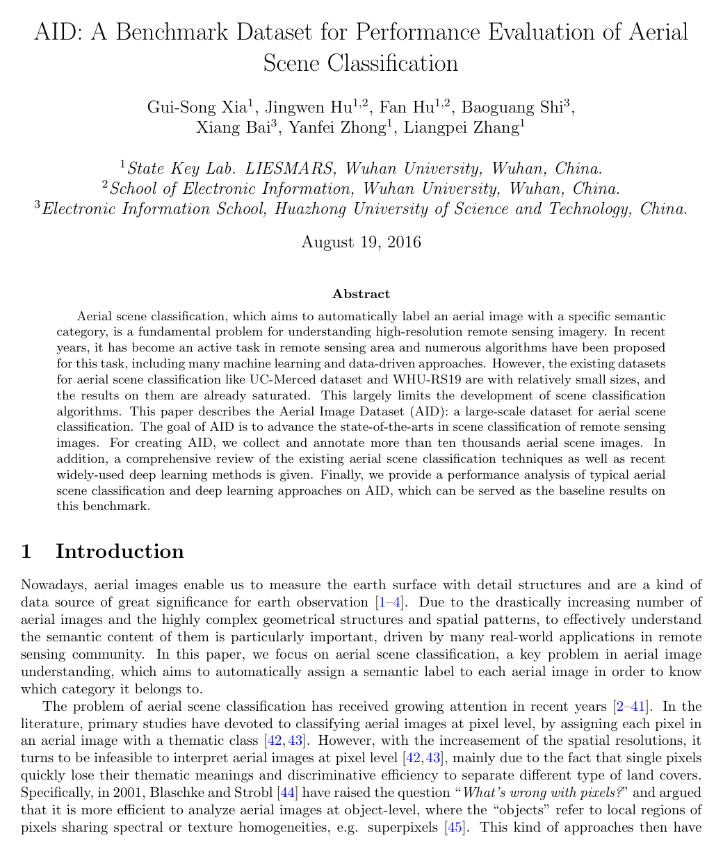
AID: A Benchmark Data Set for Performance Evaluation of Aerial Scene Classification

Gui-Song XiaJingwen HuFan HuBaoguang ShiXiang BaiYanfei ZhongLiangpei ZhangXiaoqiang Lu

article2016IEEE Transactions on Geoscience and Remote Sensing2,303 citations

Introduces the Aerial Image Dataset (AID), a large-scale benchmark of over ten thousand annotated images that overcomes performance saturation in smaller datasets by establishing baseline evaluations for deep learning models in remote sensing scene classification.

Listen

Automated aerial scene classification is critical for earth observation, urban planning, and environmental monitoring. However, development in this field has stalled because existing standard test sets are too small and lack diversity, resulting in inflated, saturated performance metrics that do not reflect real-world complexity.

The article introduces the Aerial Image Dataset, a large-scale collection of ten thousand images across thirty semantic scene categories gathered globally across different imaging conditions, resolutions, and seasons. The investigation systematically evaluates and establishes performance baselines across low-level, mid-level, and deep learning visual classification methods.

The findings show that deep neural networks significantly outperform traditional methods across all datasets, achieving overall accuracy rates near ninety percent on the new dataset, compared to thirty to thirty-seven percent for low-level features and seventy-two to seventy-nine percent for top mid-level methods. Furthermore, the new dataset exposes substantial classification challenges in newly introduced, fine-grained categories that share complex structures, such as schools versus dense residential areas and resorts versus parks, where accuracy drops to between forty-nine and sixty-five percent.

These results indicate that while deep learning provides robust feature representations, standard automated vision systems still struggle with semantic ambiguity between structurally similar land-use types. Future development must focus on advancing high-level architectures tailored to resolve fine-grained spatial distinctions in diverse, large-scale imagery.

Huazhong University of Science and Technology State Key Laboratory of Information Engineering in Surveying, Mapping and Remote Sensing Wuhan University classification algorithm classification models deep learning aerial scene classification Aerial Image Datasets Land-use scene classification

arXiv: 1608.05167

Paper: Learning Deep Features for Scene Recognition using Places Database, Bolei Zhou et al. (2014). Read this account of Places-trained deep scene features first to understand the deep-learning approach that AID evaluates against traditional visual features.
Paper: Beyond Bags of Features: Spatial Pyramid Matching for Recognizing Natural Scene Categories, Svetlana Lazebnik et al. (2006). Its spatial-pyramid method supplies an influential mid-level scene-classification baseline that helps make sense of AID’s comparisons with learned features.
Paper: A Bayesian hierarchical model for learning natural scene categories, Li Fei-Fei et al. (2005). This earlier probabilistic scene-classification approach provides useful context for the traditional methods that AID benchmarks against deep networks.
Paper: ImageNet: A large-scale hierarchical image database, Jia Deng et al. (2009). Its large-scale labeled image resource provides background on the data foundation that enabled the pretrained visual models evaluated in AID.

Paper: Remote Sensing Image Scene Classification: Benchmark and State of the Art, Gong Cheng et al. (2017). This later benchmark enlarges AID’s remote-sensing scene-classification effort with more images and categories, allowing readers to see how the field addressed its scale and diversity limits.
Paper: EuroSAT: A Novel Dataset and Deep Learning Benchmark for Land Use and Land Cover Classification, Patrick Helber et al. (2017). EuroSAT carries benchmark-based land-use classification into multispectral satellite data, extending AID’s evaluation of visual classifiers to a different Earth-observation input.
Paper: GEO-Bench: Toward Foundation Models for Earth Monitoring, Alexandre Lacoste et al. (2023). GEO-Bench continues the push for comparable Earth-observation evaluations by standardizing classification and segmentation tasks across multiple geospatial datasets.

Cover for AID: A Benchmark Data Set for Performance Evaluation of Aerial Scene Classification

Abstract

Aerial scene classification, which aims to automatically label an aerial image with a specific semantic category, is a fundamental problem for understanding high-resolution remote sensing imagery. In recent years, it has become an active task in remote sensing area and numerous algorithms have been proposed for this task, including many machine learning and data-driven approaches. However, the existing datasets for aerial scene classification like UC-Merced dataset and WHU-RS19 are with relatively small sizes, and the results on them are already saturated. This largely limits the development of scene classification algorithms. This paper describes the Aerial Image Dataset (AID): a large-scale dataset for aerial scene classification. The goal of AID is to advance the state-of-the-arts in scene classification of remote sensing images. For creating AID, we collect and annotate more than ten thousands aerial scene images. In addition, a comprehensive review of the existing aerial scene classification techniques as well as recent widely-used deep learning methods is given. Finally, we provide a performance analysis of typical aerial scene classification and deep learning approaches on AID, which can be served as the baseline results on this benchmark.

Topics

classification algorithm classification models deep learning performance analysis scene classification semantics high resolution remote sensing high resolution image foreground objects

Keywords

aerial scene classification Aerial Image Datasets Land-use scene classification High-resolution satellite scene classification local image descriptors Spatial Pyramid Matching Remote Sensing

1 Introduction
2 A review on aerial scene classification
2.1 Methods using low-level visual features
2.2 Methods relying on mid-level visual representations
2.3 Methods based on high-level vision information
3 Aerial Image Datasets (AID) for aerial scene classification
3.1 Existing datasets for aerial scene classification
3.1.1 UC-Merced dataset [57]
3.1.2 WHU-RS dataset
3.1.3 RSSCN7 dataset [40]
3.1.4 Other small datasets
3.2 AID: a new dataset for aerial scene classification
3.3 Why AID is proper for aerial image classification?
4 Baseline methods
4.1 Methods with low-level scene features
4.2 Methods with mid-level scene features
4.3 Methods with high-level scene features
5 Experimental studies
5.1 Parameter Settings
5.2 Evaluation protocols
5.3 Experimental results
5.3.1 Results with low-level methods
5.3.2 Results with mid-level methods
5.3.3 Results with high-level methods
5.3.4 Confusion matrix
5.4 Discussion
6 Conclusion
References

Knowls

Knowl 1 — Aerial Image Dataset (AID) Benchmark Specification
definition
The Aerial Image Dataset (AID) is a large-scale, multi-source, multi-resolution benchmark designed for semantic scene classification in high-resolution remote sensing.

Key specifications of the AID benchmark include:
- Scale and Classes: Comprises 10,000 RGB images categorized into 30 semantic scene types: airport, bare land, baseball field, beach, bridge, center, church, commercial, dense residential, desert, farmland, forest, industrial, meadow, medium residential, mountain, park, parking, playground, pond, port, railway station, resort, river, school, sparse residential, square, stadium, storage tanks, and viaduct.
- Class Balance: The sample count per category varies between 220 and 420 annotated images.
- Image Dimensions: Every image is fixed at a resolution of $600 \times 600$ pixels.
- Spatial Resolution Range: Ground sampling distance varies across images from approximately $0.5\text{ m}$ to $8\text{ m}$ per pixel, enabling multiscale evaluation.
- Geographic and Imaging Diversity: Sourced from Google Earth imagery across different sensor types and geographic regions (including China, the United States, England, France, Italy, Japan, and Germany) captured at varying times, seasons, sun elevation angles, and viewing directions.
- Benchmark Design Criteria: High intra-class diversity (multi-scale scene layouts, varied architectural styles, varying shadows and seasonal appearance) combined with low inter-class dissimilarity (fine-grained distinctions between visually similar categories such as playground vs. stadium, bare land vs. desert, and resort vs. park).

Knowl 2 — Class-Wise Image Distribution in the AID Benchmark

data/table

The AID dataset contains 10,000 total images partitioned across 30 aerial scene categories. The exact number of annotated image samples per category is listed in the table below.

Scene Type	Image Count	Scene Type	Image Count	Scene Type	Image Count
airport	360	farmland	370	port	380
bare land	310	forest	250	railway station	260
baseball field	220	industrial	390	resort	290
beach	400	meadow	280	river	410
bridge	360	medium residential	290	school	300
center	260	mountain	340	sparse residential	300
church	240	park	350	square	330
commercial	350	parking	390	stadium	290
dense residential	410	playground	370	storage tanks	360
desert	300	pond	420	viaduct	420

The sample size ranges from 220 (baseball field) to 420 (pond and viaduct), reflecting natural variations in scene availability while ensuring substantial sample counts per class.

Knowl 3 — Multi-Level Feature Extraction Framework for Aerial Scene Classification
model/method
Aerial scene classification models are structured across three distinct representation levels:
1. Low-Level Descriptors:
  - SIFT: Extracted on dense grayscale grids using patches of $16 \times 16$ pixels with an 8-pixel stride, generating 128-dimensional local descriptors (8 orientation bins over $4 \times 4$ spatial subregions), globally aggregated via average pooling into a single 128-dimensional image vector.
  - Local Binary Patterns (LBP): Computes 8-neighbor local binary patterns per pixel, quantizing into a 256-dimensional pattern occurrence histogram over the grayscale image.
  - Color Histogram (CH): Computes 32-bin histograms per color channel in RGB space, concatenated into a 96-dimensional global spectral descriptor.
  - GIST: Convolves the grayscale image with Gabor filters across 4 scales ( $S=4$ ) and 8 orientations ( $D=8$ ) over a $4 \times 4$ spatial pooling grid, producing a $16 \times S \times D = 512$ -dimensional spatial envelope descriptor.
2. Mid-Level Representations:
  - Combines local patch descriptors (SIFT, LBP, or CH sampled on $16 \times 16$ $16 \times 16$ grids with 8-pixel spacing) with global feature coding methods:
    - Bag of Visual Words (BoVW): Quantizes patch descriptors against a $K$ -word codebook learned via $k$ -means.
    - Spatial Pyramid Matching (SPM): Concatenates weighted multi-level ( $L=2$ ) subregion histograms to produce a $\frac{4^L - 1}{3} K$ -dimensional representation.
    - Locality-constrained Linear Coding (LLC): Projects local descriptors onto local coordinate bases using locality constraints, followed by max pooling over $K$ bases.
    - Topic Models (pLSA and LDA): Models images as probability mixtures over $T = K/2$ latent topics.
    - Improved Fisher Kernel (IFK): Encodes first- and second-order gradient statistics of a Gaussian Mixture Model (GMM) with $K$ components, yielding a $2 \cdot K \cdot F$ -dimensional vector for $F$ -dimensional patch descriptors.
    - Vector of Locally Aggregated Descriptors (VLAD): Accumulates descriptor residuals relative to nearest $k$ -means centroids, yielding a $K \cdot F$ -dimensional vector.
3. High-Level Representations:
  - Global activations extracted from the first fully-connected layer (fc6) of deep Convolutional Neural Networks pre-trained on ImageNet (ILSVRC 2012):
    - CaffeNet: 4096-dimensional activation vector.
    - VGG-VD-16: 4096-dimensional activation vector from 16 convolutional/dense layers.
    - GoogLeNet: 1024-dimensional activation vector from the final global average pooled fully connected layer.
  - High-level feature vectors are $L_2$ -normalized prior to classification.
Knowl 4 — Experimental Evaluation Protocol for Aerial Scene Classification Benchmarks
experimental setup
To evaluate aerial scene classification methods, global feature vectors are classified using a linear Support Vector Machine trained via the LIBLINEAR library.

Evaluation protocols comprise:
- Dataset Partitions:
  - AID: Evaluated under 20% training / 80% testing and 50% training / 50% testing splits.
  - UC-Merced: Evaluated under 50% training / 50% testing and 80% training / 20% testing splits.
  - WHU-RS19: Evaluated under 40% training / 60% testing and 60% training / 40% testing splits.
  - RSSCN7: Evaluated under 20% training / 80% testing and 50% training / 50% testing splits.
- Trial Repetition: Train/test splits are sampled randomly and repeated across 10 independent trials to account for variance.
- Metrics:
  - Overall Accuracy (OA): Defined as the number of correctly classified test images $N_{\text{correct}}$ divided by the total number of test images $N_{\text{total}}$ , reported as the mean $\pm$ standard deviation across 10 runs: $\text{OA} = \frac{N_{\text{correct}}}{N_{\text{total}}} \times 100\%$
  - Confusion Matrix: An $M \times M$ matrix where $M$ is the number of classes; matrix entry $x_{ij}$ measures the proportion of samples belonging to ground-truth class $j$ that are predicted as class $i$ , computed on fixed splits (50% train for UC-Merced, 40% for WHU-RS19, 20% for RSSCN7, and 20% for AID).

Knowl 5 — Classification Performance of Low-Level Visual Features on Scene Classification Benchmarks

data/table

The overall accuracy (mean $\pm$ standard deviation over 10 runs) of four low-level feature extraction methods (SIFT, LBP, Color Histogram, and GIST) evaluated across UC-Merced, WHU-RS19, RSSCN7, and AID is shown below.

Methods	UC-M (.5)	UC-M (.8)	WHU (.4)	WHU (.6)	RSSCN7 (.2)	RSSCN7 (.5)	AID (.2)	AID (.5)
SIFT	28.92 $\pm$ 0.95	32.10 $\pm$ 1.95	25.37 $\pm$ 1.32	27.21 $\pm$ 1.77	28.45 $\pm$ 1.03	32.76 $\pm$ 1.25	13.50 $\pm$ 0.67	16.76 $\pm$ 0.65
LBP	34.57 $\pm$ 1.38	36.29 $\pm$ 1.90	40.11 $\pm$ 1.46	44.08 $\pm$ 2.02	57.55 $\pm$ 1.18	60.38 $\pm$ 1.03	26.26 $\pm$ 0.52	29.99 $\pm$ 0.49
CH	42.09 $\pm$ 1.14	46.21 $\pm$ 1.05	48.79 $\pm$ 2.37	51.87 $\pm$ 3.40	57.20 $\pm$ 1.23	60.54 $\pm$ 1.01	34.29 $\pm$ 0.40	37.28 $\pm$ 0.46
GIST	44.36 $\pm$ 1.58	46.90 $\pm$ 1.76	45.65 $\pm$ 1.06	48.82 $\pm$ 3.12	49.20 $\pm$ 0.63	52.59 $\pm$ 0.71	30.61 $\pm$ 0.63	35.07 $\pm$ 0.41

Key results:

Standalone average-pooled SIFT performs worst among low-level descriptors across all benchmarks (roughly 20% lower OA than the best low-level method).
Color Histogram (CH) achieves the most consistent performance, reaching the top accuracy on WHU-RS19 ( $51.87\%$ ) and AID ( $37.28\%$ ) due to color consistency within remote sensing categories.
GIST achieves the highest accuracy on UC-Merced ( $46.90\%$ ) by capturing dominant spatial structures in dense urban scenes.
LBP performs best on RSSCN7 ( $60.38\%$ ) where homogeneous natural textures (forest, grass, field) predominate.

Knowl 6 — Dictionary Size Scaling Behavior in Mid-Level Feature Coding Schemes
empirical result
Analyzing classification accuracy as a function of dictionary size $K \in [16, 8192]$ with dense SIFT descriptors yields distinct scaling behaviors across coding methods:
- BoVW: Classification accuracy improves monotonically with dictionary size up to $K = 4096$ , where performance gains saturate. Setting $K = 4096$ provides the best performance/speed balance.
- LLC: Overall accuracy increases monotonically throughout the full range up to $K = 8192$ .
- IFK and VLAD: Classification accuracy remains stable across all dictionary sizes from $K = 16$ to $K = 8192$ . Because feature dimensionality scales as $2 K F$ for IFK and $K F$ for VLAD (where $F$ is local descriptor dimensionality), small dictionary sizes ( $K = 32$ for IFK and $K = 64$ for VLAD) minimize memory and training cost with negligible loss in accuracy.
- Topic Models (LDA, pLSA) and SPM: Performance degrades at large dictionary sizes due to model overfitting. The optimal dictionary sizes are $K = 1024$ (yielding $T = 512$ latent topics) for pLSA and LDA, and $K = 128$ for 2-level SPM.

Knowl 7 — Benchmark Performance Comparison of Mid-Level Feature Representations

data/table

The classification accuracy (mean $\pm$ standard deviation over 10 runs) of 21 mid-level feature configurations (combining local descriptors SIFT, LBP, and CH with coding methods BoVW, IFK, LDA, LLC, pLSA, SPM, and VLAD) is benchmarked across four aerial datasets.

Methods	UC-M (.5)	UC-M (.8)	WHU (.4)	WHU (.6)	RSSCN7 (.2)	RSSCN7 (.5)	AID (.2)	AID (.5)
BoVW (SIFT)	72.40 $\pm$ 1.30	75.52 $\pm$ 2.13	77.21 $\pm$ 1.92	82.58 $\pm$ 1.72	76.91 $\pm$ 0.59	81.28 $\pm$ 1.19	62.49 $\pm$ 0.53	68.37 $\pm$ 0.40
IFK (SIFT)	78.74 $\pm$ 1.65	83.02 $\pm$ 2.19	83.35 $\pm$ 1.19	87.42 $\pm$ 1.59	81.08 $\pm$ 1.21	85.09 $\pm$ 0.93	71.92 $\pm$ 0.41	78.99 $\pm$ 0.48
LDA (SIFT)	59.24 $\pm$ 1.66	61.29 $\pm$ 1.97	69.91 $\pm$ 2.23	72.18 $\pm$ 1.58	71.07 $\pm$ 0.70	73.86 $\pm$ 0.77	51.73 $\pm$ 0.73	50.81 $\pm$ 0.54
LLC (SIFT)	70.12 $\pm$ 1.09	72.55 $\pm$ 1.83	73.28 $\pm$ 1.37	78.63 $\pm$ 2.04	73.29 $\pm$ 0.63	77.11 $\pm$ 1.29	58.06 $\pm$ 0.50	63.24 $\pm$ 0.44
pLSA (SIFT)	67.55 $\pm$ 1.11	71.38 $\pm$ 1.77	73.25 $\pm$ 1.80	77.50 $\pm$ 1.20	75.25 $\pm$ 1.20	79.37 $\pm$ 0.97	56.24 $\pm$ 0.58	63.07 $\pm$ 0.48
SPM (SIFT)	56.50 $\pm$ 1.00	60.02 $\pm$ 1.06	51.82 $\pm$ 1.63	55.82 $\pm$ 1.95	64.97 $\pm$ 0.79	68.45 $\pm$ 1.01	38.43 $\pm$ 0.51	45.52 $\pm$ 0.61
VLAD (SIFT)	71.94 $\pm$ 1.36	75.98 $\pm$ 1.60	73.96 $\pm$ 2.22	79.16 $\pm$ 1.71	74.30 $\pm$ 0.74	79.34 $\pm$ 0.71	61.04 $\pm$ 0.69	68.96 $\pm$ 0.58
BoVW (LBP)	73.48 $\pm$ 1.39	78.12 $\pm$ 1.38	71.11 $\pm$ 2.72	75.89 $\pm$ 2.40	76.74 $\pm$ 0.82	81.40 $\pm$ 1.09	56.98 $\pm$ 0.55	64.31 $\pm$ 0.41
IFK (LBP)	73.11 $\pm$ 1.08	78.02 $\pm$ 1.60	71.02 $\pm$ 2.66	75.61 $\pm$ 1.86	75.18 $\pm$ 1.18	80.31 $\pm$ 1.46	60.11 $\pm$ 0.56	69.22 $\pm$ 0.72
LDA (LBP)	61.87 $\pm$ 1.92	63.40 $\pm$ 2.05	62.93 $\pm$ 2.27	67.37 $\pm$ 2.35	70.47 $\pm$ 0.87	73.63 $\pm$ 0.91	43.22 $\pm$ 0.53	41.51 $\pm$ 0.76
LLC (LBP)	67.19 $\pm$ 1.40	72.95 $\pm$ 1.46	72.89 $\pm$ 1.98	76.00 $\pm$ 0.99	73.28 $\pm$ 0.56	77.46 $\pm$ 0.86	56.11 $\pm$ 0.61	61.53 $\pm$ 0.55
pLSA (LBP)	68.84 $\pm$ 1.18	74.07 $\pm$ 1.71	66.07 $\pm$ 2.20	71.08 $\pm$ 2.11	74.94 $\pm$ 0.52	78.97 $\pm$ 1.19	49.71 $\pm$ 0.55	57.31 $\pm$ 0.58
SPM (LBP)	55.26 $\pm$ 1.34	60.52 $\pm$ 1.46	52.72 $\pm$ 0.98	56.18 $\pm$ 2.43	68.05 $\pm$ 1.30	71.26 $\pm$ 0.96	38.33 $\pm$ 0.82	44.16 $\pm$ 0.43
VLAD (LBP)	69.02 $\pm$ 0.94	74.83 $\pm$ 2.02	65.02 $\pm$ 2.80	70.29 $\pm$ 1.91	72.63 $\pm$ 0.93	77.41 $\pm$ 1.42	53.15 $\pm$ 0.61	61.19 $\pm$ 0.49
BoVW (CH)	69.80 $\pm$ 1.11	76.33 $\pm$ 2.32	63.26 $\pm$ 1.52	67.29 $\pm$ 1.55	75.07 $\pm$ 1.18	81.74 $\pm$ 0.60	49.16 $\pm$ 0.24	56.84 $\pm$ 0.45
IFK (CH)	73.87 $\pm$ 1.09	79.14 $\pm$ 1.91	70.04 $\pm$ 1.47	74.89 $\pm$ 2.25	76.86 $\pm$ 0.78	83.32 $\pm$ 0.72	59.60 $\pm$ 0.66	67.49 $\pm$ 0.81
LDA (CH)	60.15 $\pm$ 1.23	64.12 $\pm$ 1.75	55.23 $\pm$ 1.57	58.92 $\pm$ 2.56	68.11 $\pm$ 1.85	71.29 $\pm$ 1.30	38.16 $\pm$ 0.60	41.70 $\pm$ 0.80
LLC (CH)	68.62 $\pm$ 1.68	73.00 $\pm$ 1.41	64.46 $\pm$ 1.68	68.82 $\pm$ 1.94	74.12 $\pm$ 0.80	79.94 $\pm$ 0.92	53.47 $\pm$ 0.43	58.23 $\pm$ 0.49
pLSA (CH)	67.66 $\pm$ 0.92	72.88 $\pm$ 2.14	59.88 $\pm$ 1.87	63.34 $\pm$ 1.93	73.69 $\pm$ 1.60	78.79 $\pm$ 1.02	48.35 $\pm$ 0.31	55.70 $\pm$ 0.52
SPM (CH)	53.56 $\pm$ 0.94	57.17 $\pm$ 1.72	54.05 $\pm$ 1.38	56.39 $\pm$ 1.67	64.86 $\pm$ 1.26	68.24 $\pm$ 0.71	39.60 $\pm$ 0.56	44.01 $\pm$ 0.41
VLAD (CH)	67.69 $\pm$ 1.58	72.48 $\pm$ 2.24	59.53 $\pm$ 1.85	63.97 $\pm$ 2.32	72.59 $\pm$ 1.02	79.21 $\pm$ 0.87	47.94 $\pm$ 0.39	57.34 $\pm$ 0.73

Key results:

While SIFT performs poorly as a direct low-level feature, it achieves the highest performance when encoded into mid-level representations across all coding schemes.
IFK (SIFT) consistently achieves the highest overall accuracy among all 21 mid-level combinations on all benchmarks: $83.02\%$ on UC-Merced (.8), $87.42\%$ on WHU-RS19 (.6), $85.09\%$ on RSSCN7 (.5), and $78.99\%$ on AID (.5).
SPM performs worst among mid-level schemes due to rigid spatial partitioning in rotation-invariant aerial scenes.

Knowl 8 — Performance of Deep Convolutional Neural Network Features on Aerial Benchmarks

data/table

Overall classification accuracy (mean $\pm$ standard deviation over 10 runs) using off-the-shelf high-level features extracted from deep CNNs pre-trained on ImageNet (ILSVRC 2012) across the four datasets is detailed below.

Methods	UC-M (.5)	UC-M (.8)	WHU (.4)	WHU (.6)	RSSCN7 (.2)	RSSCN7 (.5)	AID (.2)	AID (.5)
CaffeNet	93.98 $\pm$ 0.67	95.02 $\pm$ 0.81	95.11 $\pm$ 1.20	96.24 $\pm$ 0.56	85.57 $\pm$ 0.95	88.25 $\pm$ 0.62	86.86 $\pm$ 0.47	89.53 $\pm$ 0.31
VGG-VD-16	94.14 $\pm$ 0.69	95.21 $\pm$ 1.20	95.44 $\pm$ 0.60	96.05 $\pm$ 0.91	83.98 $\pm$ 0.87	87.18 $\pm$ 0.94	86.59 $\pm$ 0.29	89.64 $\pm$ 0.36
GoogLeNet	92.70 $\pm$ 0.60	94.31 $\pm$ 0.89	93.12 $\pm$ 0.82	94.71 $\pm$ 1.33	82.55 $\pm$ 1.11	85.84 $\pm$ 0.92	83.44 $\pm$ 0.40	86.39 $\pm$ 0.55

Key observations:

Deep high-level features significantly outperform low- and mid-level methods across all datasets, exceeding the best mid-level method (IFK SIFT) by over $10\%$ OA on AID ( $89.64\%$ vs. $78.99\%$ under the 50% training ratio).
CaffeNet (8 layers) and VGG-VD-16 (16 layers) demonstrate comparable top performance, whereas GoogLeNet (22 layers) performs slightly worse (e.g., $86.39\%$ on AID .5). When pre-trained networks are used purely as fixed feature extractors without domain fine-tuning, deeper network activations become excessively specialized to natural ground-level object classes.
Standard deviations on AID ( $\pm 0.29\%$ to $\pm 0.47\%$ ) are much lower than on smaller datasets like UC-Merced and WHU-RS19 (up to $\pm 1.33\%$ ) due to having tenfold more evaluation samples.

Knowl 9 — Fine-Grained Semantic Ambiguity and Confusion Patterns in the AID Benchmark
empirical result
Analyzing per-class accuracy and confusion matrices obtained by high-level CNN features (CaffeNet) on AID reveals specific structural and semantic ambiguities:
- Natural Scene Discrimination: Natural scene categories with distinct textures and spectral profiles (bare land, beach, desert, forest, mountain, port) achieve near-perfect classification accuracies ranging from $0.94$ to $0.99$ .
- Resolution of Density-Based Residential Confusion: In legacy benchmarks such as UC-Merced, dense residential, medium residential, and sparse residential categories are heavily mutually confused. In AID, these categories reach accuracies between $0.90$ and $0.94$ , demonstrating that broader multi-scale sampling resolves density-based confusions.
- Challenging Newly Introduced Urban Categories:
  - School ( $0.49$ accuracy): The lowest-performing category; severely confused with dense residential due to similar building rooftop patterns and high structural density.
  - Resort ( $0.60$ accuracy): Frequently confused with park ( $0.12$ confusion rate) because both contain lush vegetation, lakes, leisure structures, and open green spaces.
  - Square ( $0.63$ accuracy) and Center ( $0.65$ accuracy): Suffer mutual confusion with each other and with commercial/parking areas due to shared open concrete plazas and surrounding retail buildings.

Coverage note — Literature review summaries of historical pixel-level, object-level, and early handcrafted remote sensing methods were omitted as they constitute background work rather than original contributions of the benchmark.

References

1.Q. Hu, W. Wu, T. Xia, Q. Yu, P. Yang, Z. Li, and Q. Song, “Exploring the use of google earth imagery and object-based methods in land use/cover mapping,” Remote Sensing, vol. 5, no. 11, pp. 6026–6042, 2013.
2.G. Cheng, J. Han, L. Guo, Z. Liu, S. Bu, and J. Ren, “Effective and efficient midlevel visual elements-oriented land-use classification using vhr remote sensing images,” IEEE Transactions on Geoscience and Remote Sensing, vol. 53, no. 8, pp. 4238–4249, 2015.
3.G. Cheng, J. Han, P. Zhou, and L. Guo, “Multi-class geospatial object detection and geographic image classification based on collection of part detectors,” ISPRS Journal of Photogrammetry and Remote Sensing, vol. 98, pp. 119–132, 2014.
4.F. Hu, G.-S. Xia, J. Hu, and L. Zhang, “Transferring deep convolutional neural networks for the scene classification of high-resolution remote sensing imagery,” Remote Sensing, vol. 7, no. 11, pp. 14 680–14 707, 2015.
5.V. Risojević and Z. Babić, “Aerial image classification using structural texture similarity,” in IEEE International Symposium on Signal Processing and Information Technology (ISSPIT). IEEE, 2011, pp. 190–195.
6.Y. Yang and S. Newsam, “Spatial pyramid co-occurrence for image classification,” in IEEE International Conference on Computer Vision (ICCV). IEEE, 2011, pp. 1465–1472.
7.G. Sheng, W. Yang, T. Xu, and H. Sun, “High-resolution satellite scene classification using a sparse coding based multiple feature combination,” International journal of remote sensing, vol. 33, no. 8, pp. 2395–2412, 2012.
8.V. Risojević and Z. Babić, “檐rientation difference descriptor for aerial image classification,” in International Conference on Systems, Signals and Image Processing (IWSSIP). IEEE, 2012, pp. 150–153.
9.F. Hu, W. Yang, J. Chen, and H. Sun, ‘Tile-level annotation of satellite images using multi-level max-margin discriminative random field,” Remote Sensing, vol. 5, no. 5, pp. 2275–2291, 2013.
10.B. Luo, S. Jiang, and L. Zhang, “Indexing of remote sensing images with different resolutions by multiple features,” IEEE Journal of Selected Topics in Applied Earth Observations and Remote Sensing, vol. 6, no. 4, pp. 1899–1912, 2013.
11.W. Shao, W. Yang, G.-S. Xia, and G. Liu, ‘A hierarchical scheme of multiple feature fusion for high-resolution satellite scene categorization,” in Computer Vision Systems. Springer, 2013, pp. 324–333.
12.W. Shao, W. Yang, and G.-S. Xia, ‘Extreme value theory-based calibration for the fusion of multiple features in high-resolution satellite scene classification,” International Journal of Remote Sensing, vol. 34, no. 23, pp. 8588–8602, 2013.
13.V. Risojevic and Z. Babic, ‘Fusion of global and local descriptors for remote sensing image classification,” IEEE Geoscience and Remote Sensing Letters, vol. 10, no. 4, pp. 836–840, 2013.
14.Y. Yang and S. Newsam, “Geographic image retrieval using local invariant features,” IEEE Transactions on Geoscience and Remote Sensing, vol. 51, no. 2, pp. 818–832, 2013.
15.B. Zhao, Y. Zhong, and L. Zhang, “Scene classification via latent dirichlet allocation using a hybrid generative/discriminative strategy for high spatial resolution remote sensing imagery,” Remote Sensing Letters, vol. 4, no. 12, pp. 1204–1213, 2013.
16.——, ‘Hybrid generative/discriminative scene classification strategy based on latent dirichlet allocation for high spatial resolution remote sensing imagery,” in IEEE International Geoscience and Remote Sensing Symposium (IGARSS). IEEE, 2013, pp. 196–199.
17.X. Zheng, X. Sun, K. Fu, and H. Wang, “Automatic annotation of satellite images via multifeature joint sparse coding with spatial relation constraint,” IEEE Geoscience and Remote Sensing Letters, vol. 10, no. 4, pp. 652–656, 2013.
18.A. Avramović and V. Risojević, “Block-based semantic classification of high-resolution multispectral aerial images,” Signal, Image and Video Processing, pp. 1–10, 2014.
19.A. M. Cheriyadat, “Unsupervised feature learning for aerial scene classification,” IEEE Transactions on Geoscience and Remote Sensing, vol. 52, no. 1, pp. 439–451, 2014.
20.R. Kusumaningrum, H. Wei, R. Manurung, and A. Murni, “Integrated visual vocabulary in latent dirichlet allocation–based scene classification for ikonos image,” Journal of Applied Remote Sensing, vol. 8, no. 1, pp. 083 690–083 690, 2014.
21.R. Negrel, D. Picard, and P.-H. Gosselin, ‘Evaluation of second-order visual features for land-use classification,” in International Workshop on Content-Based Multimedia Indexing (CBMI). IEEE, 2014, pp. 1–5.
22.L. Zhao, P. Tang, and L. Huo, ‘A 2-d wavelet decomposition-based bag-of-visual-words model for land-use scene classification,” International Journal of Remote Sensing, vol. 35, no. 6, pp. 2296–2310, 2014.
23.L.-J. Zhao, P. Tang, and L.-Z. Huo, ‘Land-use scene classification using a concentric circle-structured multiscale bag-of-visual-words model,” IEEE Journal of Selected Topics in Applied Earth Observations and Remote Sensing, vol. 7, no. 12, pp. 4620–4631, 2014.
24.Q. Zhu, Y. Zhong, and L. Zhang, ‘Multi-feature probability topic scene classifier for high spatial resolution remote sensing imagery,” in IEEE International Geoscience and Remote Sensing Symposium (IGARSS). IEEE, 2014, pp. 2854–2857.
25.S. Chen and Y. Tian, ‘Pyramid of spatial relatons for scene-level land use classification,” IEEE Transactions on Geoscience and Remote Sensing, vol. 53, no. 4, pp. 1947–1957, 2015.
26.X. Chen, T. Fang, H. Huo, and D. Li, “Measuring the effectiveness of various features for thematic information extraction from very high resolution remote sensing imagery,” IEEE Transactions on Geoscience and Remote Sensing, vol. 53, no. 9, pp. 4837–4851, 2015.
27.Y. Zhong, M. Cui, Q. Zhu, and L. Zhang, “Scene classification based on multifeature probabilistic latent semantic analysis for high spatial resolution remote sensing images,” Journal of Applied Remote Sensing, vol. 9, no. 1, pp. 095 064–095 064, 2015.
28.H. Sridharan and A. Cheriyadat, “‘Bag of lines (bol) for improved aerial scene representation,” IEEE Geoscience and Remote Sensing Letters, vol. 12, no. 3, pp. 676–680, 2015.
29.J. Hu, G.-S. Xia, F. Hu, and L. Zhang, ‘A comparative study of sampling analysis in the scene classification of optical high-spatial resolution remote sensing imagery,” Remote Sensing, vol. 7, no. 11, pp. 14 988–15 013, 2015.
30.J. Hu, T. Jiang, X. Tong, G.-S. Xia, and L. Zhang, ‘A benchmark for scene classification of high spatial resolution remote sensing imagery,” in IEEE International Geoscience and Remote Sensing Symposium (IGARSS). IEEE, 2015, pp. 5003–5006.
31.F. Hu, G.-S. Xia, Z. Wang, X. Huang, L. Zhang, and H. Sun, “Unsupervised feature learning via spectral clustering of multidimensional patches for remotely sensed scene classification,” IEEE Journal of Selected Topics in Applied Earth Observations and Remote Sensing, vol. 8, no. 5, pp. 2015–2030, 2015.
32.M. Castelluccio, G. Poggi, C. Sansone, and L. Verdoliva, ‘Land use classification in remote sensing images by convolutional neural networks,” arXiv preprint arXiv:1508.00092, 2015.
33.O. A. B. Penatti, K. Nogueira, and J. A. dos Santos, “Do deep features generalize from everyday objects to remote sensing and aerial scenes domains?” in Proc. IEEE Conference on Computer Vision and Pattern Recognition, June 2015.
34.F. Luus, B. Salmon, F. van den Bergh, and B. Maharaj, ‘Multiview deep learning for land-use classification,” IEEE Geoscience and Remote Sensing Letters, vol. 12, no. 12, pp. 2448–2452, 2015.
35.W. Yang, X. Yin, and G.-S. Xia, ‘Learning high-level features for satellite image classification with limited labeled samples,” IEEE Transactions on Geoscience and Remote Sensing, vol. 53, no. 8, pp. 4472–4482, 2015.
36.F. Zhang, B. Du, and L. Zhang, ‘Saliency-guided unsupervised feature learning for scene classification,” IEEE Transactions on Geoscience and Remote Sensing, vol. 53, no. 4, pp. 2175–2184, 2015.
37.——, “Scene classification via a gradient boosting random convolutional network framework,” IEEE Transactions on Geoscience and Remote Sensing, vol. PP, no. 99, pp. 1–10, 2015.
38.Y. Zhong, Q. Zhu, and L. Zhang, ‘Scene classification based on the multifeature fusion probabilistic topic model for high spatial resolution remote sensing imagery,” IEEE Transactions on Geoscience and Remote Sensing, vol. 53, no. 11, pp. 6207–6222, 2015.
39.C. Chen, B. Zhang, H. Su, W. Li, and L. Wang, ‘Land-use scene classification using multi-scale completed local binary patterns,” Signal, Image and Video Processing, pp. 1–8, 2015.
40.Q. Zou, L. Ni, T. Zhang, and Q. Wang, ‘Deep learning based feature selection for remote sensing scene classification,” Geoscience and Remote Sensing Letters, IEEE, vol. 12, no. 11, pp. 2321–2325, 2015.
41.K. Nogueira, O. A. Penatti, and J. A. d. Santos, “檐owards better exploiting convolutional neural networks for remote sensing scene classification,” arXiv preprint arXiv:1602.01517, 2016.
42.D. Tuia, F. Ratle, F. Pacifici, M. F. Kanevski, and W. J. Emery, “Active learning methods for remote sensing image classification,” IEEE Transactions on Geoscience and Remote Sensing, vol. 47, no. 7, pp. 2218–2232, 2009.
43.D. Tuia, M. Volpi, L. Copa, M. Kanevski, and J. Muqoz-Marı, ‘A survey of active learning algorithms for supervised remote sensing image classification,” IEEE Journal of Selected Topics in Signal Processing, vol. 5, no. 3, pp. 606–617, 2011.
44.T. Blaschke and J. Strobl, “Whats wrong with pixels? some recent developments interfacing remote sensing and gis,” GeoBIT/GIS, vol. 6, no. 01, pp. 12–17, 2001.
45.N. B. Kotliar and J. A. Wiens, “檐ultiple scales of patchiness and patch structure: a hierarchical framework for the study of heterogeneity,” Oikos, pp. 253–260, 1990.
46.T. Blaschke, “檐bject-based contextual image classification built on image segmentation,” in IEEE Workshop on Advances in Techniques for Analysis of Remotely Sensed Data. IEEE, 2003, pp. 113–119.
47.G. Yan, J.-F. Mas, B. Maathuis, Z. Xiangmin, and P. Van Dijk, “Comparison of pixel-based and object-oriented image classification approachesa case study in a coal fire area, wuda, inner mongolia, china,” International Journal of Remote Sensing, vol. 27, no. 18, pp. 4039–4055, 2006.
48.T. Blaschke, “檐bject based image analysis for remote sensing,” ISPRS journal of photogrammetry and remote sensing, vol. 65, no. 1, pp. 2–16, 2010.
49.S. W. Myint, P. Gober, A. Brazel, S. Grossman-Clarke, and Q. Weng, “Per-pixel vs. object-based classification of urban land cover extraction using high spatial resolution imagery,” Remote sensing of environment, vol. 115, no. 5, pp. 1145–1161, 2011.
50.D. C. Duro, S. E. Franklin, and M. G. Dube, ‘A comparison of pixel-based and object-based image analysis with selected machine learning algorithms for the classification of agricultural landscapes using spot-5 hrg imagery,” Remote Sensing of Environment, vol. 118, pp. 259–272, 2012.
51.Y. Zhong, J. Zhao, and L. Zhang, ‘A hybrid object-oriented conditional random field classification framework for high spatial resolution remote sensing imagery,” IEEE Transactions on Geoscience and Remote Sensing, vol. 52, no. 11, pp. 7023–7037, 2014.
52.J. Zhao, Y. Zhong, and L. Zhang, ‘Detail-preserving smoothing classifier based on conditional random fields for high spatial resolution remote sensing imagery,” IEEE Transactions on Geoscience and Remote Sensing, vol. 53, no. 5, pp. 2440–2452, 2015.
53.Y. Yang and S. Newsam, ‘Comparing sift descriptors and gabor texture features for classification of remote sensed imagery,” in IEEE International Conference on Image Processing. IEEE, 2008, pp. 1852–1855.
54.J. A. dos Santos, O. A. B. Penatti, and R. da Silva Torres, “檐valuating the potential of texture and color descriptors for remote sensing image retrieval and classification.” in VISAPP (2), 2010, pp. 203–208.
55.M. Lienou, H. Maˆıtre, and M. Datcu, “檐emantic annotation of satellite images using latent dirichlet allocation,” IEEE Geoscience and Remote Sensing Letters, vol. 7, no. 1, pp. 28–32, 2010.
56.G.-S. Xia, W. Yang, J. Delon, Y. Gousseau, H. Sun, and H. Maˆıtre, “Structural high-resolution satellite image indexing,” in ISPRS TC VII Symposium-100 Years ISPRS, vol. 38, 2010, pp. 298–303.
57.Y. Yang and S. Newsam, ‘Bag-of-visual-words and spatial extensions for land-use classification,” in Proceedings of the 18th SIGSPATIAL International Conference on Advances in Geographic Information Systems. ACM, 2010, pp. 270–279.
58.L. Chen, W. Yang, K. Xu, and T. Xu, “檐valuation of local features for scene classification using vhr satellite images,” in Joint Urban Remote Sensing Event (JURSE). IEEE, 2011, pp. 385–388.
59.D. Dai and W. Yang, “‘Satellite image classification via two-layer sparse coding with biased image representation,” IEEE Geoscience and Remote Sensing Letters, vol. 8, no. 1, pp. 173–176, 2011.
60.V. Risojević, S. Momić, and Z. Babić, ‘Gabor descriptors for aerial image classification,” in Adaptive and Natural Computing Algorithms. Springer, 2011, pp. 51–60.
61.A. Oliva and A. Torralba, “檐odeling the shape of the scene: A holistic representation of the spatial envelope,” International Journal of Computer Vision, vol. 42, no. 3, pp. 145–175, 2001.
62.D. G. Lowe, “檐istinctive image features from scale-invariant keypoints,” International Journal of Computer Vision, vol. 60, no. 2, pp. 91–110, 2004.
63.M. J. Swain and D. H. Ballard, “檐olor indexing,” International journal of computer vision, vol. 7, no. 1, pp. 11–32, 1991.
64.B. S. Manjunath and W.-Y. Ma, ‘Texture features for browsing and retrieval of image data,” IEEE Transactions on Pattern Analysis and Machine Intelligence, vol. 18, no. 8, pp. 837–842, 1996.
65.T. Ojala, M. Pietik¨ainen, and T. M¨aenp¨a¨a, ‘Multiresolution gray-scale and rotation invariant texture classification with local binary patterns,” IEEE Transactions on Pattern Analysis and Machine Intelligence, vol. 24, no. 7, pp. 971–987, 2002.
66.B. Luo, J.-F. Aujol, Y. Gousseau, and S. Ladjal, “‘Indexing of satellite images with different resolutions by wavelet features,” IEEE Transactions on Image Processing, vol. 17, no. 8, pp. 1465–1472, 2008.
67.B. Luo, J.-F. Aujol, and Y. Gousseau, ‘Local scale measure from the topographic map and application to remote sensing images,” Multiscale modeling & simulation, vol. 8, no. 1, pp. 1–29, 2009.
68.S. Mallat and L. Sifre, “Combined scattering for rotation invariant texture analysis,” submitted to ESANN, 2012.
69.W. J. Scheirer, N. Kumar, P. N. Belhumeur, and T. E. Boult, “檐ulti-attribute spaces: Calibration for attribute fusion and similarity search,” in IEEE Conference on Computer Vision and Pattern Recognition. IEEE, 2012, pp. 2933–2940.
70.J. Yang, K. Yu, Y. Gong, and T. Huang, “‘Linear spatial pyramid matching using sparse coding for image classification,” in Proc. IEEE Conference on Computer Vision and Pattern Recognition, 2009, pp. 1794–1801.
71.F. Perronnin, J. Sanchez, and T. Mensink, ‘Improving the fisher kernel for large-scale image classification,” in Proc. European Conference on Computer Vision, 2010, pp. 143–156.
72.S. Lazebnik, C. Schmid, and J. Ponce, “檐eyond bags of features: Spatial pyramid matching for recognizing natural scene categories,” in Proc. IEEE Conference on Computer Vision and Pattern Recognition, vol. 2, 2006, pp. 2169–2178.
73.D. M. Blei, A. Y. Ng, and M. I. Jordan, “檐atent dirichlet allocation,” the Journal of Machine Learning research, vol. 3, pp. 993–1022, 2003.
74.M. A. Stricker and M. Orengo, “‘Similarity of color images,” in IS&T/SPIE’s Symposium on Electronic Imaging: Science & Technology. International Society for Optics and Photonics, 1995, pp. 381–392.
75.R. M. Haralick, K. Shanmugam, and I. H. Dinstein, ‘Textural features for image classification,” IEEE Transactions on Systems, Man and Cybernetics, no. 6, pp. 610–621, 1973.
76.A. Bosch, A. Zisserman, and X. Muqoz, “Scene classification via plsa,” in Proc. European Conference on Computer Vision, 2006, pp. 517–530.
77.P. Vincent, H. Larochelle, I. Lajoie, Y. Bengio, and P.-A. Manzagol, “Stacked denoising autoencoders: Learning useful representations in a deep network with a local denoising criterion,” The Journal of Machine Learning Research, vol. 11, pp. 3371–3408, 2010.
78.O. Russakovsky, J. Deng, H. Su, J. Krause, S. Satheesh, S. Ma, Z. Huang, A. Karpathy, A. Khosla, M. Bernstein, A. C. Berg, and L. Fei-Fei, “ImageNet Large Scale Visual Recognition Challenge,” International Journal of Computer Vision, pp. 1–42, April 2015.
79.P. Sermanet, D. Eigen, X. Zhang, M. Mathieu, R. Fergus, and Y. LeCun, ‘Overfeat: Integrated recognition, localization and detection using convolutional networks,” arXiv preprint arXiv:1312.6229, 2013.
80.Y. Jia, E. Shelhamer, J. Donahue, S. Karayev, J. Long, R. Girshick, S. Guadarrama, and T. Darrell, “affe: Convolutional architecture for fast feature embedding,” in Proceedings of the ACM International Conference on Multimedia. ACM, 2014, pp. 675–678.
81.C. Szegedy, W. Liu, Y. Jia, P. Sermanet, S. Reed, D. Anguelov, D. Erhan, V. Vanhoucke, and A. Rabinovich, “Going deeper with convolutions,” arXiv preprint arXiv:1409.4842, 2014.
82.J. Sivic and A. Zisserman, “Video google: A text retrieval approach to object matching in videos,” in Proc. IEEE International Conference on Computer Vision, 2003, pp. 1470–1477.
83.H. Jegou, F. Perronnin, M. Douze, J. Sanchez, P. Perez, and C. Schmid, ‘Aggregating local image descriptors into compact codes,” IEEE Transactions on Pattern Analysis and Machine Intelligence, vol. 34, no. 9, pp. 1704–1716, 2012.
84.G. E. Hinton, S. Osindero, and Y. W. Teh, ‘A fast learning algorithm for deep belief nets.” Neural Computation, vol. 18, no. 7, pp. 1527–54, 2006.
85.J. Wang, J. Yang, K. Yu, F. Lv, T. Huang, and Y. Gong, ‘Locality-constrained linear coding for image classification,” in Proc. IEEE Conference on Computer Vision and Pattern Recognition. IEEE, 2010, pp. 3360–3367.
86.K. Yu, T. Zhang, and Y. Gong, “‘Nonlinear learning using local coordinate coding,” in Advances in Neural Information Processing Systems, 2009, pp. 2223–2231.
87.F. Perronnin and C. Dance, ‘Fisher kernels on visual vocabularies for image categorization,” in Proc. IEEE Conference on Computer Vision and Pattern Recognition. IEEE, 2007, pp. 1–8.
88.A. Krizhevsky, I. Sutskever, and G. E. Hinton, ‘Imagenet classification with deep convolutional neural networks,” in Advances in Neural Information Processing Systems, 2012, pp. 1097–1105.
89.K. Simonyan and A. Zisserman, ‘Very deep convolutional networks for large-scale image recognition,” CoRR, vol. abs/1409.1556, 2014.
90.L. Min, C. Qiang, and S. Yan, “Network in network,” CoRR, vol. abs/1312.4400, 2013.
91.R. E. Fan, K. W. Chang, C. J. Hsieh, X. R. Wang, and C. J. Lin, “檐iblinear: A library for large linear classification,” Journal of Machine Learning Research, vol. 9, no. 12, pp. 1871–1874, 2010.

Citation

MLA

Xia, G.-S., et al. “AID: A Benchmark Data Set for Performance Evaluation of Aerial Scene Classification”. IEEE Transactions on Geoscience and Remote Sensing, vol. 55, no. 7, 2017, pp. 3965–81, https://doi.org/10.1109/TGRS.2017.2685945.

APA

Xia, G.-S., Hu, J., Hu, F., Shi, B., Bai, X., Zhong, Y., Zhang, L., & Lu, X. (2017). AID: A Benchmark Data Set for Performance Evaluation of Aerial Scene Classification. IEEE Transactions on Geoscience and Remote Sensing, 55(7), 3965–3981. https://doi.org/10.1109/TGRS.2017.2685945

Chicago

Xia, G.-S., J. Hu, F. Hu, et al. 2017. “AID: A Benchmark Data Set for Performance Evaluation of Aerial Scene Classification”. IEEE Transactions on Geoscience and Remote Sensing 55 (7): 3965–81. https://doi.org/10.1109/TGRS.2017.2685945.

Harvard

Xia, G.-S. et al. (2017) “AID: A Benchmark Data Set for Performance Evaluation of Aerial Scene Classification”, IEEE Transactions on Geoscience and Remote Sensing, 55(7), pp. 3965–3981. Available at: https://doi.org/10.1109/TGRS.2017.2685945.

Vancouver

1. Xia G-S, Hu J, Hu F, Shi B, Bai X, Zhong Y, Zhang L, Lu X (2017) AID: A Benchmark Data Set for Performance Evaluation of Aerial Scene Classification. IEEE Transactions on Geoscience and Remote Sensing 55:3965–3981

BibTeX

@article{Xia_2017, title={AID: A Benchmark Data Set for Performance Evaluation of Aerial Scene Classification}, volume={55}, ISSN={1558-0644}, url={http://dx.doi.org/10.1109/TGRS.2017.2685945}, DOI={10.1109/tgrs.2017.2685945}, number={7}, journal={IEEE Transactions on Geoscience and Remote Sensing}, publisher={Institute of Electrical and Electronics Engineers (IEEE)}, author={Xia, Gui-Song and Hu, Jingwen and Hu, Fan and Shi, Baoguang and Bai, Xiang and Zhong, Yanfei and Zhang, Liangpei and Lu, Xiaoqiang}, year={2017}, month=July, pages={3965–3981} }

Metadata:Crossref

Access the Paper

This paper is available from its original source. Click below to access the PDF.

Open PDF

AID: A Benchmark Data Set for Performance Evaluation of Aerial Scene Classification

Abstract

Topics

Keywords

Table of Contents

Knowls

Knowl 1 — Aerial Image Dataset (AID) Benchmark Specification

Knowl 2 — Class-Wise Image Distribution in the AID Benchmark

Knowl 3 — Multi-Level Feature Extraction Framework for Aerial Scene Classification

Knowl 4 — Experimental Evaluation Protocol for Aerial Scene Classification Benchmarks

Knowl 5 — Classification Performance of Low-Level Visual Features on Scene Classification Benchmarks

Knowl 6 — Dictionary Size Scaling Behavior in Mid-Level Feature Coding Schemes

Knowl 7 — Benchmark Performance Comparison of Mid-Level Feature Representations

Knowl 8 — Performance of Deep Convolutional Neural Network Features on Aerial Benchmarks

Knowl 9 — Fine-Grained Semantic Ambiguity and Confusion Patterns in the AID Benchmark

References

Citation

BibTeX

Access the Paper