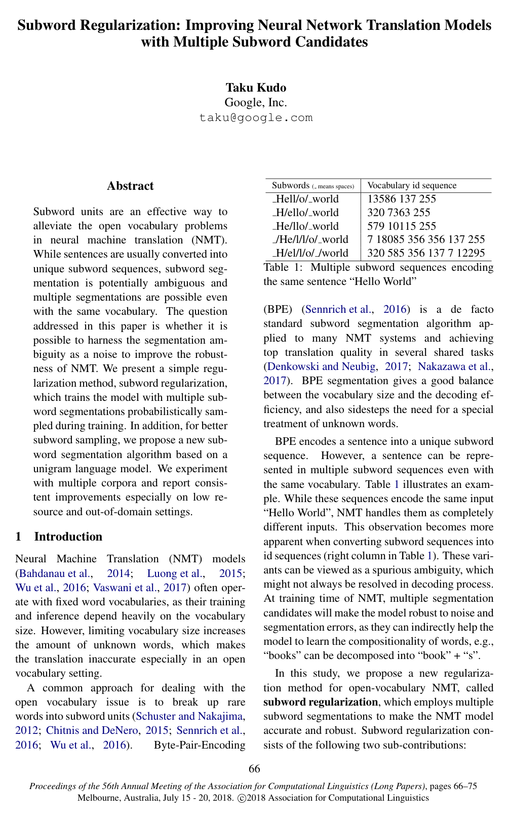
Subword Regularization: Improving Neural Network Translation Models with Multiple Subword Candidates

Taku Kudo

article2018ACL1,410 citations

Proposes a unigram language model segmentation algorithm and a subword regularization technique that probabilistically samples multiple segmentations during training, significantly improving neural machine translation on low-resource and out-of-domain tasks.

Listen

Standard neural machine translation systems convert text into subword units to handle large and open vocabularies efficiently. However, standard methods like Byte-Pair Encoding rely on deterministic segmentations that assign a single subword sequence to each sentence, ignoring alternative valid segmentations. This lack of flexibility makes translation models fragile when exposed to real-world noise, rare words, or unfamiliar domains.

The article introduces and evaluates "subword regularization," a training method designed to enhance translation accuracy and robustness by exposing models to multiple subword candidates during training. It also proposes a probabilistic unigram language model to generate and sample these subword variations according to their likelihood.

To evaluate this approach, the authors conducted translation experiments across multiple datasets of varying sizes (from small corpora of roughly 133,000 sentences to large corpora exceeding 15 million sentences) covering diverse languages such as English, Vietnamese, Chinese, French, Arabic, Japanese, German, and Czech. The method samples alternative subword sequences on-the-fly during training without altering the underlying neural network architecture. Translation performance was measured using standard translation quality benchmark scores (BLEU) across both standard test sets and out-of-domain datasets (such as Web text, patents, and query logs).

The evaluation yielded several key findings. First, subword regularization delivered consistent translation quality improvements of 1 to 2 BLEU points over standard baseline methods across nearly all language pairs. Second, the performance gains were most pronounced in low-resource language settings (such as small benchmark datasets) and in out-of-domain evaluations, where quality improvements reached up to roughly 2 to 10 BLEU points even for models trained on massive datasets. Third, combining subword regularization with multi-candidate search during translation (n-best decoding) provided additional quality gains. Finally, applying regularization to both the source and target sentences yielded the largest benefits, though applying it to either side individually still showed positive effects.

These findings indicate that introducing probabilistic segmentation noise acts as an effective data augmentation strategy, teaching models how words are composed and making them significantly more resilient to unfamiliar inputs. Because subword regularization operates purely through data sampling, it requires no structural redesign of machine translation models, minimizing technical complexity and implementation risk while delivering meaningful quality improvements.

Organizations developing or deploying translation systems should adopt probabilistic subword segmentation to improve robustness, particularly when working with limited training data or user-generated, open-domain content. When implementing the approach, practitioners should tune sampling hyperparameters using validation datasets, choosing moderate candidate sizes (such as 64 candidates) for high-resource settings to prevent over-regularization. Future efforts should also explore applying this technique to other sequence-generation applications, such as dialogue systems and text summarization.

Confidence in these findings is high across diverse languages and domains, though hyperparameter sensitivity represents an operational limitation: choosing completely uniform sampling without probabilistic weighting degrades performance, meaning sampling parameters must be calibrated carefully.

Google language model neural networks regularization methods subword regularization neural machine translation subword segmentation

arXiv: 1804.10959 google/sentencepiece

Paper: Neural Machine Translation of Rare Words with Subword Units, Rico Sennrich et al. (2016). Introduces the foundational use of subword units via byte pair encoding (BPE) to solve the open-vocabulary problem in neural machine translation, which this paper directly improves upon.
Paper: Effective Approaches to Attention-based Neural Machine Translation, Minh-Thang Luong et al. (2015). Establishes standard attention-based encoder-decoder architectures for neural machine translation, serving as the base translation framework regularized in this work.
Paper: Neural Machine Translation by Jointly Learning to Align and Translate, Dzmitry Bahdanau et al. (2015). Introduces the attention mechanism for sequence-to-sequence neural translation that underpins the baseline models evaluated in this research.
Paper: Enriching Word Vectors with Subword Information, Piotr Bojanowski et al. (2017). Demonstrates the power of character and subword n-gram representations for capturing morphology, motivating the transition toward richer subword vocabularies.
Paper: Character-Aware Neural Language Models, Yoon Kim et al. (2015). Explores character-level compositionality in neural language modeling to overcome fixed word-level vocabulary constraints.
Paper: Recurrent Neural Network Regularization, Wojciech Zaremba et al. (2014). Presents foundational dropout techniques for regularizing sequence models, establishing the broader regularization paradigm that subword regularization complements.

Paper: SentencePiece: A simple and language independent subword tokenizer and detokenizer for Neural Text Processing, Taku Kudo et al. (2018). Directly implements and generalizes the unigram language model subword segmentation and regularization algorithms introduced in this work into the widely used SentencePiece toolkit.
Paper: Cross-lingual Language Model Pretraining, Guillaume Lample et al. (2019). Applies shared subword vocabularies and unsupervised tokenization schemes to cross-lingual pre-training for downstream machine translation and language understanding.
Paper: Multilingual Denoising Pre-training for Neural Machine Translation, Yinhan Liu et al. (2020). Extends subword-tokenized sequence modeling to large-scale multilingual denoising pre-training across 25 languages for low-resource translation.
Paper: Teaching Old Tokenizers New Words: Efficient Tokenizer Adaptation for Pre-trained Models, Taido Purason et al. (2025). Explores subsequent methods for dynamically adapting and pruning pre-trained subword tokenizers when transferring models to new languages or domains.

Cover for Subword Regularization: Improving Neural Network Translation Models with Multiple Subword Candidates

Abstract

Subword units are an effective way to alleviate the open vocabulary problems in neural machine translation (NMT). While sentences are usually converted into unique subword sequences, subword segmentation is potentially ambiguous and multiple segmentations are possible even with the same vocabulary. The question addressed in this paper is whether it is possible to harness the segmentation ambiguity as a noise to improve the robustness of NMT. We present a simple regularization method, subword regularization, which trains the model with multiple subword segmentations probabilistically sampled during training. In addition, for better subword sampling, we propose a new subword segmentation algorithm based on a unigram language model. We experiment with multiple corpora and report consistent improvements especially on low resource and out-of-domain settings.

Topics

language model neural networks regularization methods translation models vocabulary segmentation methods

Keywords

subword regularization neural machine translation subword segmentation subword sampling encoder-decoder architectures rare words open vocabulary

1 Introduction
2 Neural Machine Translation with multiple subword segmentations
2.1 NMT training with on-the-fly subword sampling
2.2 Decoding
3 Subword segmentations with language model
3.1 Byte-Pair-Encoding (BPE)
3.2 Unigram language model
3.3 Subword sampling
3.4 BPE vs. Unigram language model
4 Related Work
5 Experiments
5.1 Setting
5.2 Main Results
5.3 Results with out-of-domain corpus
5.4 Comparison with other segmentation algorithms
5.5 Impact of sampling hyperparameters
5.6 Results with single side regularization
6 Conclusions
References

Knowls

Knowl 1 — Subword Regularization Objective and On-the-Fly Sampling
model/method
Neural machine translation (NMT) models translate a source subword sequence $\mathbf{x} = (x_1, \dots, x_M)$ to a target subword sequence $\mathbf{y} = (y_1, \dots, y_N)$ parametrized by $\theta$ via the conditional probability:

$P(\mathbf{y}|\mathbf{x}; \theta) = \prod_{n=1}^N P(y_n | \mathbf{x}, y_{<n}; \theta)$

Standard maximum likelihood estimation maximizes the log-likelihood over a parallel training corpus $D = \{ \langle X^{(s)}, Y^{(s)} \rangle \}_{s=1}^{|D|}$ of raw sentences with deterministic subword segmentations:

$\mathcal{L}(\theta) = \sum_{s=1}^{|D|} \log P(\mathbf{y}^{(s)} | \mathbf{x}^{(s)}; \theta)$

Subword regularization treats subword segmentation as a probabilistic variable. Let $P(\mathbf{x}|X)$ and $P(\mathbf{y}|Y)$ denote the probability distributions over possible segmentations of raw sentences $X$ and $Y$ , respectively. Subword regularization optimizes $\theta$ with respect to the marginalized log-likelihood:

$\mathcal{L}_{\text{marginal}}(\theta) = \sum_{s=1}^{|D|} \mathbb{E}_{\mathbf{x} \sim P(\mathbf{x}|X^{(s)}), \, \mathbf{y} \sim P(\mathbf{y}|Y^{(s)})} \left[ \log P(\mathbf{y}|\mathbf{x}; \theta) \right]$

Because exact summation over all segmentations is computationally intractable, the expectation is approximated by drawing $k$ segmentation samples per sentence:

$\mathcal{L}_{\text{marginal}}(\theta) \cong \frac{1}{k^2} \sum_{s=1}^{|D|} \sum_{i=1}^k \sum_{j=1}^k \log P(\mathbf{y}_j | \mathbf{x}_i; \theta), \quad \mathbf{x}_i \sim P(\mathbf{x}|X^{(s)}), \; \mathbf{y}_j \sim P(\mathbf{y}|Y^{(s)})$

In online mini-batch training with a large number of update iterations, setting $k = 1$ and sampling a new subword segmentation on-the-fly for each parameter update provides an efficient and effective approximation of the marginal objective.
Knowl 2 — Unigram Language Model for Probabilistic Subword Segmentation
model/method
The unigram language model for subword segmentation assumes that subword units occur independently. Given a vocabulary $V$ of subword tokens, the probability of a subword sequence $\mathbf{x} = (x_1, \dots, x_M)$ is formulated as:

$P(\mathbf{x}) = \prod_{i=1}^M p(x_i), \quad \text{subject to } \forall x \in V, \, p(x) \ge 0 \text{ and } \sum_{x \in V} p(x) = 1$

where $p(x_i)$ is the occurrence probability of subword token $x_i \in V$ .

Given an input raw sentence $X$ and its set of valid segmentations $S(X)$ formed from subwords in $V$ , the most probable segmentation $\mathbf{x}^*$ is given by:

$\mathbf{x}^* = \arg\max_{\mathbf{x} \in S(X)} P(\mathbf{x})$

This optimal segmentation $\mathbf{x}^*$ is obtained in linear time using the Viterbi dynamic programming algorithm.

For a fixed vocabulary $V$ , the occurrence probabilities $\{p(x)\}_{x \in V}$ are estimated from a training corpus $D = \{X^{(s)}\}_{s=1}^{|D|}$ by maximizing the marginal likelihood $\mathcal{L}$ via the Expectation-Maximization (EM) algorithm, treating segmentations as hidden variables:

$\mathcal{L} = \sum_{s=1}^{|D|} \log P(X^{(s)}) = \sum_{s=1}^{|D|} \log \left( \sum_{\mathbf{x} \in S(X^{(s)})} P(\mathbf{x}) \right)$
Knowl 3 — Iterative Vocabulary Pruning for Unigram Subword Modeling
algorithm
The vocabulary generation algorithm jointly identifies the subword vocabulary $V$ and estimates subword occurrence probabilities $p(x)$ from a raw monolingual corpus by iteratively pruning a large initial seed vocabulary.
Input: Training corpus $D = \{X^{(s)}\}_{s=1}^{|D|}$ , target vocabulary size $V_{\text{target}}$ , pruning retention rate $\eta \in (0, 1)$ (e.g., $\eta = 0.80$ )
Output: Subword vocabulary $V$ and occurrence probabilities $\{p(x)\}_{x \in V}$
Initialize seed vocabulary $V$ :
    Extract all single characters occurring in $D$
    Enumerate frequent substrings not crossing word boundaries using Enhanced Suffix Array (in $O(T)$ time and $O(20T)$ space for corpus length $T$ )
     $V \leftarrow (\text{all characters in } D) \cup (\text{frequent substrings})$
while $|V| > V_{\text{target}}$ do
    Run EM algorithm on $D$ using current vocabulary $V$ to estimate $\{p(x)\}_{x \in V}$ maximizing $\mathcal{L} = \sum_{s=1}^{|D|} \log \left( \sum_{\mathbf{x} \in S(X^{(s)})} \prod_{x_i \in \mathbf{x}} p(x_i) \right)$
    for each subword $x_i \in V$ do
        Compute $\text{loss}_i = \mathcal{L} - \mathcal{L}_{V \setminus \{x_i\}}$ , representing the likelihood decrease when $x_i$ is removed from $V$
    end for
    Sort subwords in $V$ in descending order of $\text{loss}_i$
     $V_{\text{keep}} \leftarrow \text{top } \eta\% \text{ of subwords in } V \text{ according to } \text{loss}_i$
     $V \leftarrow V_{\text{keep}} \cup (\text{all single-character subwords})$
    if $|V| < V_{\text{target}}$ then
         $V \leftarrow \text{top } V_{\text{target}} \text{ subwords by } \text{loss}_i \cup (\text{all single-character subwords})$
    end if
end while
Run EM algorithm on $D$ using final vocabulary $V$ to obtain final $\{p(x)\}_{x \in V}$
return $V, \{p(x)\}_{x \in V}$
Single-character subwords are explicitly preserved throughout all pruning iterations to ensure that any arbitrary string can be tokenized without generating out-of-vocabulary symbols.
Knowl 4 — Probabilistic Subword Sampling via l-Best and Forward-Filtering Backward-Sampling
algorithm
Subword regularization samples subword segmentations during training from the unigram language model distribution using either an approximate $l$ -best multinomial distribution or exact dynamic programming over all possible segmentations ( $l = \infty$ ) via Forward-Filtering and Backward-Sampling (FFBS).
Input: Input raw sentence $X$ , subword unigram model $(V, p)$ , candidate size $l \in \mathbb{N}^+ \cup \{\infty\}$ , smoothing constant $\alpha > 0$
Output: Sampled subword sequence $\mathbf{x} = (x_1, \dots, x_M)$
if $l < \infty$ then
    Find the $l$ -best segmentations $\mathbf{x}_1, \dots, \mathbf{x}_l \in S(X)$ according to $P(\mathbf{x}|X)$ using Forward-DP Backward-A* search
    Compute multinomial sampling probabilities:
         $P(\mathbf{x}_i | X) = \frac{P(\mathbf{x}_i)^\alpha}{\sum_{j=1}^l P(\mathbf{x}_j)^\alpha} \quad \text{for } i \in \{1, \dots, l\}$
    Sample $\mathbf{x} \sim \text{Multinomial}(P(\mathbf{x}_1 | X), \dots, P(\mathbf{x}_l | X))$
    return $\mathbf{x}$
else
    Construct subword lattice for sentence $X$ where nodes $0, \dots, |X|$ represent character boundaries
    Forward pass: Compute forward lattice values $\alpha_{\text{fwd}}(t)$ for $t \in [0, |X|]$ :
         $\alpha_{\text{fwd}}(0) \leftarrow 1$
        for $t \leftarrow 1$ to $|X|$ do
             $\alpha_{\text{fwd}}(t) \leftarrow \sum_{w = X[s:t] \in V} \alpha_{\text{fwd}}(s) \cdot p(w)^\alpha$
        end for
    Backward pass: Recursively sample subwords from end to beginning:
         $t \leftarrow |X|$
         $\mathbf{x} \leftarrow []$
        while $t > 0$ do
            For each incoming subword $w = X[s:t] \in V$ , compute transition probability:
                 $P_{\text{trans}}(s \to t) = \frac{\alpha_{\text{fwd}}(s) \cdot p(w)^\alpha}{\alpha_{\text{fwd}}(t)}$
            Sample start index $s$ according to $P_{\text{trans}}(s \to t)$
            Prepend subword $w = X[s:t]$ to $\mathbf{x}$
             $t \leftarrow s$
        end while
    return $\mathbf{x}$
end if
The hyperparameter $\alpha$ controls distribution smoothness: smaller $\alpha$ yields a more uniform distribution, whereas larger $\alpha$ biases sampling toward the Viterbi segmentation $\mathbf{x}^*$ .
Knowl 5 — Decoding Strategies with Multiple Subword Segmentations
model/method
At inference time, an NMT model trained with subword regularization can translate an input sentence $X$ using either 1-best decoding or $n$ -best decoding:
1. 1-Best Decoding: The input sentence $X$ is segmented deterministically into its most probable segmentation $\mathbf{x}^* = \arg\max_{\mathbf{x} \in S(X)} P(\mathbf{x})$ , and the target sequence is generated by beam search conditioned on $\mathbf{x}^*$ .
2. $n$ -Best Decoding: The top $n$ segmentation candidates $(\mathbf{x}_1, \dots, \mathbf{x}_n)$ of $X$ are obtained from the unigram language model distribution $P(\mathbf{x}|X)$ . For each candidate $\mathbf{x}_i$ , translation hypothesis $\mathbf{y}_i$ is generated, and the optimal output $\mathbf{y}^*$ is selected to maximize the length-penalized score:
$\operatorname{score}(\mathbf{x}, \mathbf{y}) = \frac{\log P(\mathbf{y}|\mathbf{x})}{|\mathbf{y}|^\lambda}$

where $|\mathbf{y}|$ is the number of subwords in hypothesis $\mathbf{y}$ , and $\lambda \in \mathbb{R}^+$ is a length penalty parameter tuned on development data.

$n$ -best decoding provides consistent improvements over 1-best decoding when subword regularization is used during training, but degrades translation quality if the model was trained without subword regularization ( $l=1$ ), because the decoder is unprepared for non-deterministic segmentations.

Knowl 6 — In-Domain Machine Translation BLEU Performance Across Languages

data/table

The table below summarizes translation quality (BLEU %) across multiple language pairs and dataset sizes using Google's Neural Machine Translation (GNMT) architecture. The comparison includes Byte-Pair-Encoding (BPE), deterministic Unigram language model ( $l = 1$ ), and Unigram with Subword Regularization (SR) under candidate sampling ( $l = 64, \alpha = 0.1$ ) and full lattice sampling ( $l = \infty, \alpha = 0.2$ for IWSLT and $\alpha = 0.5$ for other corpora), evaluated under both 1-best and $n$ -best decoding ( $n = 64$ ).

		Baseline	Proposed (1-best decoding)			Proposed ( $n$ -best decoding, $n=64$ )
Corpus	Pair	(BPE)	$l=1$	$l=64, \alpha=0.1$	$l=\infty, \alpha=0.2/0.5$	$l=1$	$l=64, \alpha=0.1$	$l=\infty, \alpha=0.2/0.5$
IWSLT15	en $\rightarrow$ vi	25.61	25.49	27.68*	27.71*	25.33	28.18*	28.48*
	vi $\rightarrow$ en	22.48	22.32	24.73*	26.15*	22.04	24.66*	26.31*
	en $\rightarrow$ zh	16.70	16.90	19.36*	20.33*	16.73	20.14*	21.30*
	zh $\rightarrow$ en	15.76	15.88	17.79*	16.95*	16.23	17.75*	17.29*
IWSLT17	en $\rightarrow$ fr	35.53	35.39	36.70*	36.36*	35.16	37.60*	37.01*
	fr $\rightarrow$ en	33.81	33.74	35.57*	35.54*	33.69	36.07*	36.06*
	en $\rightarrow$ ar	13.01	13.04	14.92*	15.55*	12.29	14.90*	15.36*
	ar $\rightarrow$ en	25.98	27.09*	28.47*	29.22*	27.08*	29.05*	29.29*
KFTT	en $\rightarrow$ ja	27.85	28.92*	30.37*	30.01*	28.55*	31.46*	31.43*
	ja $\rightarrow$ en	21.37	21.46	22.33*	22.04*	21.37	22.47*	22.64*
ASPEC	en $\rightarrow$ ja	40.62	40.66	41.24*	41.23*	40.86	41.55*	41.87*
	ja $\rightarrow$ en	26.51	26.76	27.08*	27.14*	27.49*	27.75*	27.89*
WMT14	en $\rightarrow$ de	24.53	24.50	25.04*	24.74	22.73	25.00*	24.57
	de $\rightarrow$ en	28.01	28.65*	28.83*	29.39*	28.24	29.13*	29.97*
	en $\rightarrow$ cs	25.25	25.54	25.41	25.26	24.88	25.49	25.38
	cs $\rightarrow$ en	28.78	28.84	29.64*	29.41*	25.77	29.23*	29.15*

Asterisks (*) indicate statistically significant differences ( $p < 0.05$ ) from the BPE baseline by bootstrap resampling.

Without subword regularization ( $l = 1$ ), the Unigram model performs similarly to BPE. Enabling subword regularization ( $l > 1$ ) yields statistically significant improvements of +1 to +2 BLEU across nearly all language pairs, with larger gains in low-resource settings (IWSLT, KFTT). $n$ -best decoding yields further gains only when combined with subword regularization.

Knowl 7 — Out-of-Domain Translation Robustness with Subword Regularization

data/table

To evaluate generalization under domain shifts, NMT models trained on in-domain parallel corpora (IWSLT15, IWSLT17, and WMT14) were evaluated on out-of-domain datasets comprising Web (5k sentences), Patent (2k sentences), and Query log (2k sentences) genres using 1-best decoding ( $l = \infty, \alpha = 0.2$ for IWSLT; $l = 64, \alpha = 0.1$ for WMT14).

Domain	Training Corpus	Language Pair	Baseline (BPE)	Proposed (SR)
Web (5k)	IWSLT15	en $\rightarrow$ vi	13.86	17.36*
		vi $\rightarrow$ en	7.83	11.69*
		en $\rightarrow$ zh	9.71	13.85*
		zh $\rightarrow$ en	5.93	8.13*
	IWSLT17	en $\rightarrow$ fr	16.09	20.04*
		fr $\rightarrow$ en	14.77	19.99*
	WMT14	en $\rightarrow$ de	22.71	26.02*
		de $\rightarrow$ en	26.42	29.63*
		en $\rightarrow$ cs	19.53	21.41*
		cs $\rightarrow$ en	25.94	27.86*
Patent (2k)	WMT14	en $\rightarrow$ de	15.63	25.76*
		de $\rightarrow$ en	22.74	32.66*
		en $\rightarrow$ cs	16.70	19.38*
		cs $\rightarrow$ en	23.20	25.30*
Query (2k)	IWSLT15	en $\rightarrow$ zh	9.30	12.47*
		zh $\rightarrow$ en	14.94	19.99*
	IWSLT17	en $\rightarrow$ fr	10.79	10.99
		fr $\rightarrow$ en	19.01	23.96*
	WMT14	en $\rightarrow$ de	25.93	29.82*
		de $\rightarrow$ en	26.24	30.90*

Asterisks (*) indicate statistically significant differences ( $p < 0.05$ ) from the BPE baseline by bootstrap resampling.

Subword regularization achieves substantial BLEU improvements (+2 to +10 points) across out-of-domain corpora. Notably, strong improvements occur even for models trained on large datasets (such as WMT14 en $\leftrightarrow$ de and en $\leftrightarrow$ cs), where in-domain gains were modest, indicating that subword regularization improves translation robustness against unknown words and domain mismatch.

Knowl 8 — Comparison Across Tokenization and Subword Segmentation Algorithms

data/table

Translation performance (BLEU %) on the WMT14 English-to-German (en $\rightarrow$ de) benchmark using different text representation and segmentation approaches with GNMT:

Model	BLEU (%)
Word	23.12
Character (512 nodes)	22.62
Mixed Word/Character	24.17
Byte-Pair-Encoding (BPE)	24.53
Unigram w/o Subword Regularization ( $l = 1$ )	24.50
Unigram w/ Subword Regularization ( $l = 64, \alpha = 0.1$ )	25.04

Word-level models suffer from vocabulary size limits on morphologically rich languages like German, lagging subword models by more than 1 BLEU point. Without regularization, the unigram language model performs identically to BPE (24.50 vs. 24.53 BLEU). Subword regularization with on-the-fly sampling ( $l = 64, \alpha = 0.1$ ) achieves the highest translation quality (25.04 BLEU), outperforming deterministic subword segmentation and mixed word/character models.

Knowl 9 — Sensitivity and Behavior of Sampling Hyperparameters
empirical result
The effectiveness of subword regularization depends on the candidate set size $l$ and the distribution smoothing parameter $\alpha$ :
1. Necessity of Biased Sampling: Setting $\alpha = 0.0$ (sampling subword segmentations uniformly, ignoring language model probabilities $P(\mathbf{x}|X)$ ) leads to severe performance degradation, performing worse than the deterministic baseline, especially when sampling from the full lattice ( $l = \infty$ ). Sampling must be biased by subword occurrence probabilities to emulate realistic morphological variation.
2. Interaction Between $l$ and $\alpha$ : Full lattice sampling ( $l = \infty$ ) searches an exponentially larger candidate space than $l = 64$ , requiring a larger smoothing constant (e.g., $\alpha = 0.2$ to $0.5$ ) to keep sampled sequences reasonably close to the Viterbi path $\mathbf{x}^*$ . For candidate-restricted sampling ( $l = 64$ ), peak performance occurs at smaller smoothing values (e.g., $\alpha = 0.1$ ).
3. Resource Regimes: While $l = \infty$ enables more aggressive data augmentation and yields higher peak BLEU scores on low-resource datasets (e.g., IWSLT), it is more sensitive to $\alpha$ tuning. Setting $l = 64$ provides more robust and stable regularization for higher-resource corpora.

Knowl 10 — Source-Side, Target-Side, and Joint Subword Regularization

data/table

Translation results (BLEU %) on IWSLT datasets evaluating the effect of applying subword regularization ( $l = 64, \alpha = 0.1$ ) to the source sentence only (encoder), the target sentence only (decoder), or both:

Regularization Type	en $\rightarrow$ vi	vi $\rightarrow$ en	en $\rightarrow$ ar	ar $\rightarrow$ en
No regularization (baseline, $l=1$ )	25.49	22.32	13.04	27.09
Source only	26.00	23.09*	13.46	28.16*
Target only	26.10	23.62*	14.34*	27.89*
Source and target (full SR)	27.68*	24.73*	14.92*	28.47*

Asterisks (*) indicate statistically significant differences ( $p < 0.05$ ) from the unregularized baseline by bootstrap resampling.

While applying subword regularization to both source and target sentences achieves the highest BLEU scores, single-sided regularization (either encoder-only or decoder-only) consistently outperforms the unregularized baseline across all language pairs. This demonstrates that subword regularization is beneficial not only for full encoder-decoder translation models, but also for standalone encoder architectures (e.g., text classification) and standalone decoder architectures (e.g., language modeling).

Coverage note — None was omitted; all primary methodological contributions, algorithms (unigram vocabulary pruning and sampling), decoding formulations, main empirical benchmark results, domain robustness experiments, ablation studies, and hyperparameter analyses are fully covered.

References

1.Mikel Artetxe, Gorka Labaka, Eneko Agirre, and Kyunghyun Cho. 2017. Unsupervised neural machine translation. arXive preprint arXiv:1710.11041 .
2.Dzmitry Bahdanau, Kyunghyun Cho, and Yoshua Bengio. 2014. Neural machine translation by jointly learning to align and translate. arXiv preprint arXiv:1409.0473 .
3.Yonatan Belinkov and Yonatan Bisk. 2017. Synthetic and natural noise both break neural machine translation. arXive preprint arXiv:1711.02173 .
4.William Chan, Yu Zhang, Quoc Le, and Navdeep Jaitly. 2016. Latent sequence decompositions. arXiv preprint arXiv:1610.03035 .
5.Rohan Chitnis and John DeNero. 2015. Variable-length word encodings for neural translation models. In Proc. of EMNLP. pages 2088–2093.
6.Michael Denkowski and Graham Neubig. 2017. Stronger baselines for trustable results in neural machine translation. Proc. of Workshop on Neural Machine Translation .
7.Philip Gage. 1994. A new algorithm for data compression. C Users J. 12(2):23–38.
8.Jonas Gehring, Michael Auli, David Grangier, Denis Yarats, and Yann N Dauphin. 2017. Convolutional sequence to sequence learning. arXiv preprint arXiv:1705.03122 .
9.Ian Goodfellow, Jonathon Shlens, and Christian Szegedy. 2015. Explaining and harnessing adversarial examples. In Proc. of ICLR.
10.Mohit Iyyer, Varun Manjunatha, Jordan Boyd-Graber, and Hal Daume III. 2015. Deep unordered composition rivals syntactic methods for text classification. In Proc. of ACL.
11.Diederik P Kingma and Jimmy Ba Adam. 2014. A method for stochastic optimization. arXiv preprint arXiv:1412.6980 .
12.Philipp Koehn. 2004. Statistical significance tests for machine translation evaluation. In Proc. of EMNLP.
13.Guillaume Lample, Ludovic Denoyer, and Marc’Aurelio Ranzato. 2017. Unsupervised machine translation using monolingual corpora only. arXive preprint arXiv:1711.00043 .
14.Minh-Thang Luong, Hieu Pham, and Christopher D Manning. 2015. Effective approaches to attention-based neural machine translation. In Proc of EMNLP.
15.Masaaki Nagata. 1994. A stochastic japanese morphological analyzer using a forward-dp backward-a* n-best search algorithm. In Proc. of COLING.
16.Toshiaki Nakazawa, Shohei Higashiyama, Chenchen Ding, Hideya Mino, Isao Goto, Hideto Kazawa, Yusuke Oda, Graham Neubig, and Sadao Kurohashi. 2017. Overview of the 4th workshop on asian translation. In Proceedings of the 4th Workshop on Asian Translation (WAT2017). pages 1–54.
17.Ge Nong, Sen Zhang, and Wai Hong Chan. 2009. Linear suffix array construction by almost pure induced-sorting. In Proc. of DCC.
18.Kishore Papineni, Salim Roukos, Todd Ward, and Wei-Jing Zhu. 2002. Bleu: a method for automatic evaluation of machine translation. In Proc. of ACL.
19.Alexander M Rush, Sumit Chopra, and Jason Weston. 2015. A neural attention model for abstractive sentence summarization. In Proc. of EMNLP.
20.Mike Schuster and Kaisuke Nakajima. 2012. Japanese and korean voice search. In Proc. of ICASSP.
21.Steven L Scott. 2002. Bayesian methods for hidden markov models: Recursive computing in the 21st century. Journal of the American Statistical Association .
22.Rico Sennrich, Barry Haddow, and Alexandra Birch. 2016. Neural machine translation of rare words with subword units. In Proc. of ACL.
23.Matthias Sperber, Graham Neubig, Jan Niehues, and Alex Waibel. 2017. Neural lattice-to-sequence models for uncertain inputs. In Proc. of EMNLP.
24.Nitish Srivastava, Geoffrey E Hinton, Alex Krizhevsky, Ilya Sutskever, and Ruslan Salakhutdinov. 2014. Dropout: a simple way to prevent neural networks from overfitting. JMLR 15(1).
25.Jinsong Su, Zhixing Tan, De yi Xiong, Rongrong Ji, Xiaodong Shi, and Yang Liu. 2017. Lattice-based recurrent neural network encoders for neural machine translation. In AAAI. pages 3302–3308.
26.Kai Sheng Tai, Richard Socher, and Christopher D Manning. 2015. Improved semantic representations from tree-structured long short-term memory networks. Proc. of ACL .
27.Ashish Vaswani, Noam Shazeer, Niki Parmar, Jakob Uszkoreit, Llion Jones, Aidan N. Gomez, Lukasz Kaiser, and Illia Polosukhin. 2017. Attention is all you need. arXive preprint arXiv:1706.03762 .
28.Pascal Vincent, Hugo Larochelle, Yoshua Bengio, and Pierre-Antoine Manzagol. 2008. Extracting and composing robust features with denoising autoencoders. In Proc. of ICML.
29.Oriol Vinyals and Quoc V. Le. 2015. A neural conversational model. In ICML Deep Learning Workshop.
30.Oriol Vinyals, Alexander Toshev, Samy Bengio, and Dumitru Erhan. 2015. Show and tell: A neural image caption generator. In Computer Vision and Pattern Recognition.
31.Andrew Viterbi. 1967. Error bounds for convolutional codes and an asymptotically optimum decoding algorithm. IEEE transactions on Information Theory 13(2):260–269.
32.Yonghui Wu, Mike Schuster, et al. 2016. Google’s neural machine translation system: Bridging the gap between human and machine translation. arXiv preprint arXiv:1609.08144 .
33.Ziang Xie, Sida I. Wang, Jiwei Li, Daniel Levy, Aiming Nie, Dan Jurafsky, and Andrew Y. Ng. 2017. Data noising as smoothing in neural network language models. In Proc. of ICLR.

Citation

MLA

Kudo, T. “Subword Regularization: Improving Neural Network Translation Models with Multiple Subword Candidates”. arXiv, 2018, http://arxiv.org/abs/1804.10959v1.

APA

Kudo, T. (2018). Subword Regularization: Improving Neural Network Translation Models with Multiple Subword Candidates. arXiv. http://arxiv.org/abs/1804.10959v1

Chicago

Kudo, T. 2018. “Subword Regularization: Improving Neural Network Translation Models with Multiple Subword Candidates”. arXiv. http://arxiv.org/abs/1804.10959v1.

Harvard

Kudo, T. (2018) “Subword Regularization: Improving Neural Network Translation Models with Multiple Subword Candidates”, arXiv [Preprint]. Available at: http://arxiv.org/abs/1804.10959v1.

Vancouver

1. Kudo T (2018) Subword Regularization: Improving Neural Network Translation Models with Multiple Subword Candidates. arXiv

BibTeX

@article{kudo2018subword,
  title = {Subword Regularization: Improving Neural Network Translation Models with Multiple Subword Candidates},
  author = {Kudo, Taku},
  year = {2018},
  journal = {arXiv},
  url = {http://arxiv.org/abs/1804.10959v1},
  eprint = {1804.10959}
}

Metadata:arXiv

Source Code

This paper has an official code repository available. Click below to access the source code.

View Repository

Access the Paper

This paper is available from its original source. Click below to access the PDF.

Open PDF

License: https://creativecommons.org/licenses/by/4.0/

Subword Regularization: Improving Neural Network Translation Models with Multiple Subword Candidates

Abstract

Topics

Keywords

Table of Contents

Knowls

Knowl 1 — Subword Regularization Objective and On-the-Fly Sampling

Knowl 2 — Unigram Language Model for Probabilistic Subword Segmentation

Knowl 3 — Iterative Vocabulary Pruning for Unigram Subword Modeling

Knowl 4 — Probabilistic Subword Sampling via l-Best and Forward-Filtering Backward-Sampling

Knowl 5 — Decoding Strategies with Multiple Subword Segmentations

Knowl 6 — In-Domain Machine Translation BLEU Performance Across Languages

Knowl 7 — Out-of-Domain Translation Robustness with Subword Regularization

Knowl 8 — Comparison Across Tokenization and Subword Segmentation Algorithms

Knowl 9 — Sensitivity and Behavior of Sampling Hyperparameters

Knowl 10 — Source-Side, Target-Side, and Joint Subword Regularization

References

Citation

BibTeX

Source Code

Access the Paper