Ray tracing volume densities

James T. KajiyaBrian P. Von Herzen

article1984SIGGRAPH1,505 citations

Presents the foundational ray tracing algorithms and radiative transfer solutions for rendering participating media such as clouds, fog, and flames defined within 3D volume grids.

Listen

Synthesizing realistic imagery of participating media and natural atmospheric phenomena—such as clouds, fog, flames, and dust—presents a major challenge in computer graphics. Earlier rendering techniques relied on restrictive plane-parallel models, low-reflectance assumptions, or fixed viewing and lighting geometries that fail when generating general, dynamic scenes.

The article demonstrates a generalized ray tracing framework capable of rendering arbitrary three-dimensional volume densities and introduces a mathematical approximation to handle multiple light scattering in highly reflective media like clouds.

The approach models volume densities on uniform 3D grids and splits the rendering workflow into two distinct stages: a precomputation phase that maps illumination through the volume, and an execution phase that integrates ray brightness and optical depth during ray tracing. To overcome the computational intractability of full radiative transfer, the authors develop a perturbation method expanded in spherical harmonics and truncate it to low orders. Additionally, they simulate cloud density evolution using a physical atmospheric convection model governed by partial differential equations.

The article establishes several key findings. First, single-scattering approximations cause severe visual defects, specifically artificial darkening on the shadowed sides of clouds, proving that realistic rendering of high-reflectance media requires accounting for multiple scattering. Second, separating the illumination precomputation from ray traversal allows unrestricted camera angles, internal viewing, and scene interactions such as cloud-induced shadows and reflections in other objects. Third, the spherical harmonic perturbation approach decouples directional scattering effectively, enabling numerical relaxation for high-reflectance scenarios. Finally, physically simulated convection grids (tested on 10x10x20 meshes) successfully generate dynamically realistic cloud formations across multi-minute lifespans, with render times ranging from 1 to 4 hours per frame on an IBM 4341.

These findings mean that computer-generated imagery can represent complex natural phenomena and particle systems without restrictive geometry, enhancing realism in visual simulations and animation. However, the computational cost remains high, requiring significant processing time per frame, and the current framework has a limitation where procedural objects do not cast reciprocal shadows back into the volume densities.

Teams implementing volumetric rendering should adopt precalculated illumination grids for ray tracing efficiency and apply low-order spherical harmonic approximations for bright scattering media. Future development should focus on optimizing grid computation, supporting bidirectional shadowing between solids and volumes, and evaluating higher-resolution physical simulations.

  • Paper: The rendering equation, James T. Kajiya (1986). Kajiya formalizes the general rendering equation that generalizes early surface and volume scattering formulations into a unified framework solved via Monte Carlo path tracing.
  • Paper: Marching cubes: A high resolution 3D surface construction algorithm, William E. Lorensen et al. (1987). Lorensen and Cline introduce the marching cubes algorithm to extract explicit isosurfaces directly from the 3D volumetric density grids discussed in volume rendering.
  • Paper: Stable fluids, Jos Stam (1999). Stam develops an unconditionally stable numerical framework to simulate dynamic fluid and smoke advection through 3D density grids, substantially advancing dynamic volume modeling.
  • Paper: 3D Gaussian Splatting for Real-Time Radiance Field Rendering, Bernhard Kerbl et al. (2023). Kerbl et al. modernize volume and radiance field rendering by leveraging 3D Gaussian primitives to enable real-time novel view synthesis from volumetric representations.
  • Paper: TensoRF: Tensorial Radiance Fields, Anpei Chen et al. (2022). Chen et al. extend volumetric radiance and density fields through tensorial grid decompositions to dramatically accelerate volume reconstruction and rendering.
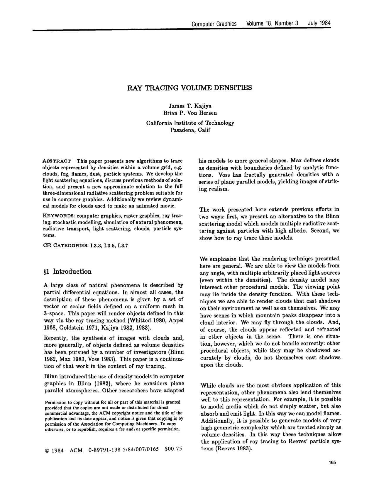
Cover for Ray tracing volume densities

Abstract

This paper presents new algorithms to trace objects represented by densities within a volume grid, e.g. clouds, fog, flames, dust, particle systems. We develop the light scattering equations, discuss previous methods of solution, and present a new approximate solution to the full three-dimensional radiative scattering problem suitable for use in computer graphics. Additionally we review dynamical models for clouds used to make an animated movie.

Table of Contents

  • §1 Introduction
  • §2 The scattering equation
  • §3 Solving the scattering equation
  • 3.1 Blinn's Low Albedo approximation
  • 3.2 A ray tracing algorithm for the low albedo case
  • §4 High Albedo approximation.
  • 4.1 A Perturbation solution, conservative systems
  • 4.2 The Scattering equation expressed in Spherical Harmonics
  • 4.3 Matrix elements for the position
  • 4.4 Matrix elements for the phase integral
  • §5 Generating density models
  • 5.1 A Cloud Model for Generating Density Functions
  • §6 Computer Results
  • §7 Summary
  • §8 References

Knowls

  1. Knowl 1 — Two-Pass Ray Tracing Algorithm for Volume Densities

    algorithm

    The two-pass volume rendering algorithm computes the single-scattering radiance of volume densities on a 3D grid, allowing arbitrary viewing angles, internal/external light sources, and intersections with solid procedural geometry.

    Input: Density grid ρ(x,y,z)\rho(x,y,z), extinction coefficient τ\tau, phase function p(cos⁡Θ)p(\cos\Theta), light sources {Li}\{L_i\}, camera ray parameters, solid scene database
    Output: Pixel radiance BB
    // Pass 1: Precompute light illumination array (performed at most once per frame)
    for each light source ii do
        for each grid element (x,y,z)(x,y,z) in volume extent do
            Compute ray path Γx,y,z(t)=(x(t),y(t),z(t))\Gamma_{x,y,z}(t) = (x(t), y(t), z(t)) from light ii to (x,y,z)(x,y,z)
            Ii(x,y,z)←exp⁡(−τ∫Γx,y,zρ(γ) dγ)I_i(x,y,z) \leftarrow \exp\left(-\tau \int_{\Gamma_{x,y,z}} \rho(\gamma)\,d\gamma\right)
        end for
    end for
    // Pass 2: Ray trace eye rays
    for each viewing ray R(t)=(x(t),y(t),z(t))R(t) = (x(t), y(t), z(t)) from the eye do
        Intersect R(t)R(t) with volume bounding box to get entry distance d1d_1 and exit distance d2d_2
        Intersect R(t)R(t) with solid scene geometry to get nearest solid intersection distance dglobald_{\text{global}}
        λ1←max⁡(0,d1)\lambda_1 \leftarrow \max(0, d_1)
        λ2←min⁡(dglobal,d2)\lambda_2 \leftarrow \min(d_{\text{global}}, d_2)
        if λ1<λ2\lambda_1 < \lambda_2 then
            Evaluate the brightness integral over [λ1,λ2][\lambda_1, \lambda_2] using Romberg numerical integration:
            B←∫λ1λ2exp⁡(−τ∫λ1tρ(x(μ),y(μ),z(μ)) dμ)⋅[∑iIi(x(t),y(t),z(t))p(cos⁡Θi)]⋅ρ(x(t),y(t),z(t)) dtB \leftarrow \int_{\lambda_1}^{\lambda_2} \exp\left(-\tau \int_{\lambda_1}^t \rho(x(\mu), y(\mu), z(\mu))\,d\mu\right) \cdot \left[\sum_i I_i(x(t), y(t), z(t)) p(\cos\Theta_i)\right] \cdot \rho(x(t), y(t), z(t))\,dt
        else
            B←0B \leftarrow 0
        end if
        Composite BB with light reflected from solid surface at dglobald_{\text{global}}
    end for

    The inner line integral ∫λ1tρ dμ\int_{\lambda_1}^t \rho\,d\mu computes the optical depth between the viewer and the scattering element, while Ii(x(t),y(t),z(t))I_i(x(t), y(t), z(t)) provides the precomputed incident light attenuation from source ii to that point. The phase angle Θi\Theta_i is the angle between the incoming light direction and the ray direction towards the eye.

  2. Knowl 2 — Radiative Transfer Scattering Equation for Volume Densities

    equation

    The radiative transfer equation governing the intensity field I(x,s)I(x, s) at position x∈R3x \in \mathbb{R}^3 along direction unit vector ss (where ∥s∥=1\|s\| = 1) in a participating medium with local density ρ(x)\rho(x), optical depth per unit density κ\kappa, and no intrinsic thermal emission is:

    −1κρ(x)s⋅∇xI(x,s)−I(x,s)+14π∫∥s~∥=1p(s,s~)I(x,s~) ds~=0-\frac{1}{\kappa \rho(x)} s \cdot \nabla_x I(x, s) - I(x, s) + \frac{1}{4\pi} \int_{\|\tilde{s}\|=1} p(s, \tilde{s}) I(x, \tilde{s}) \, d\tilde{s} = 0

    where:

    • s⋅∇xI(x,s)=dIdss \cdot \nabla_x I(x, s) = \frac{dI}{ds} is the directional derivative of intensity along the direction ss.
    • κρ(x)\kappa \rho(x) is the local extinction coefficient.
    • p(s,s~)p(s, \tilde{s}) is the scattering phase function defining the proportion of light scattered from incident direction s~\tilde{s} into direction ss.
    • For isotropic media, p(s,s~)p(s, \tilde{s}) depends only on the phase angle Θ\Theta between ss and s~\tilde{s} (where cos⁡Θ=s⋅s~\cos\Theta = s \cdot \tilde{s}), with perfectly diffuse scattering given by p(cos⁡Θ)=ω0p(\cos\Theta) = \omega_0 and Rayleigh scattering given by p(cos⁡Θ)=34ω0(1+cos⁡2Θ)p(\cos\Theta) = \frac{3}{4}\omega_0(1 + \cos^2\Theta), where ω0\omega_0 is the single-scattering albedo.
  3. Knowl 3 — Perturbation Expansion for High-Albedo Volume Radiative Transfer

    model/method

    For high-albedo scattering media (such as clouds where single-scattering albedo ω0≈1\omega_0 \approx 1), standard Neumann series expansions converge slowly. The solution is obtained via a perturbation expansion in the absorption parameter β=1−ω0\beta = 1 - \omega_0.

    Normalizing the phase function by p(Θ)=ω0pˉ(Θ)=(1−β)pˉ(Θ)p(\Theta) = \omega_0 \bar{p}(\Theta) = (1 - \beta)\bar{p}(\Theta), the radiative transfer equation is expressed in operator form:

    LI+(1−β)MI=0L I + (1 - \beta) M I = 0

    where the linear operators are defined as:

    LI=−1κρ(x)s⋅∇xI(x,s)−I(x,s)L I = -\frac{1}{\kappa \rho(x)} s \cdot \nabla_x I(x, s) - I(x, s)

    MI=14π∫∥s~∥=1pˉ(s,s~)I(x,s~) ds~M I = \frac{1}{4\pi} \int_{\|\tilde{s}\|=1} \bar{p}(s, \tilde{s}) I(x, \tilde{s}) \, d\tilde{s}

    Expanding the radiation intensity into a power series in β\beta,

    I=∑k=0∞βkIkI = \sum_{k=0}^\infty \beta^k I_k

    and matching equal powers of β\beta yields a recursive sequence of forced conservative (ω0=1\omega_0 = 1) scattering equations:

    LIk+MIk=−MIk−1L I_k + M I_k = -M I_{k-1}

    where I−1=0I_{-1} = 0.

  4. Knowl 4 — Spherical Harmonics Representation and P-Wave Truncation for Radiative Transfer

    model/method

    The angular dependence of the intensity field I(x,s)I(x, s) is expanded in normalized spherical harmonics Ylm(s)=Plm(cos⁡θ)eimϕY_{lm}(s) = P_{lm}(\cos\theta) e^{im\phi}:

    I(x,s)=∑l=0∞∑m=−llIlm(x)Ylm(s)I(x, s) = \sum_{l=0}^\infty \sum_{m=-l}^l I^{lm}(x) Y_{lm}(s)

    where PlmP_{lm} are the associated Legendre polynomials of degree ll and order mm. Projecting the radiative transfer equation onto each spherical harmonic basis function using the inner product ⟨X∣O∣Y⟩=∫02π∫0πX∗(s)OY(s)sin⁡θ dθ dϕ\langle X | O | Y \rangle = \int_0^{2\pi} \int_0^\pi X^*(s) O Y(s) \sin\theta \, d\theta \, d\phi produces a coupled system of first-order partial differential equations for the spatial intensity coefficients Ilm(x)I^{lm}(x):

    ∑l,m1κρ(x)∇Ilm(x)⋅⟨Yl′m′(s)∣s∣Ylm(s)⟩−Il′m′(x)+∑l,mIlm(x)⟨Yl′m′(s)∣p∣Ylm(s)⟩=0\sum_{l, m} \frac{1}{\kappa \rho(x)} \nabla I^{lm}(x) \cdot \langle Y_{l'm'}(s) | s | Y_{lm}(s) \rangle - I^{l'm'}(x) + \sum_{l, m} I^{lm}(x) \langle Y_{l'm'}(s) | p | Y_{lm}(s) \rangle = 0

    For computer graphics rendering, the spherical harmonic series is truncated at degree l=1l = 1 ("p-wave" truncation). This retains four spatial fields (l=0,m=0l=0, m=0 and l=1,m=−1,0,1l=1, m=-1,0,1), reducing the high-dimensional angular transport problem to a small system of coupled 3D PDEs solvable across the volume grid by numerical relaxation.

  5. Knowl 5 — Matrix Elements for Direction and Phase Operators in Spherical Harmonics

    theoretical result

    Projection of the radiative transport operators onto the spherical harmonic basis YlmY_{lm} yields exact coupling matrix elements:

    1. Direction Operator ss: Using the complex variable u=x+iy=sin⁡θeiϕu = x + iy = \sin\theta e^{i\phi} and z=cos⁡θz = \cos\theta:

    ⟨Yl′m′(s)∣u∣Ylm(s)⟩=(k0δl′,l+1−k1δl′,l−1)δm′,m+1⋅2π\langle Y_{l'm'}(s) | u | Y_{lm}(s) \rangle = (k_0 \delta_{l', l+1} - k_1 \delta_{l', l-1}) \delta_{m', m+1} \cdot 2\pi

    where k0=(l−m+1)(l−m+2)2l+1k_0 = \frac{(l - m + 1)(l - m + 2)}{2l + 1} and k1=(l+m−1)(l+m)2l+1k_1 = \frac{(l + m - 1)(l + m)}{2l + 1}. For the zz-component:

    ⟨Yl′m′(s)∣z∣Ylm(s)⟩=(k2δl′,l+1−k3δl′,l−1)δm′m⋅2π\langle Y_{l'm'}(s) | z | Y_{lm}(s) \rangle = (k_2 \delta_{l', l+1} - k_3 \delta_{l', l-1}) \delta_{m' m} \cdot 2\pi

    where k2=l+m2l+1k_2 = \frac{l + m}{2l + 1} and k3=l−m+12l+1k_3 = \frac{l - m + 1}{2l + 1}. Consequently, the spatial gradient operator couples only adjacent spherical harmonic degrees l±1l \pm 1.

    1. Phase Function Operator pp: Expanding an isotropic phase function p(cos⁡Θ)p(\cos\Theta) in Legendre polynomials p(cos⁡Θ)=∑k=0∞wkPk(cos⁡Θ)p(\cos\Theta) = \sum_{k=0}^\infty w_k P_k(\cos\Theta) and applying Laplace's addition theorem yields:

    ⟨Yl′m′(s)∣p∣Ylm(s)⟩=4π2l+1wlδll′δmm′\langle Y_{l'm'}(s) | p | Y_{lm}(s) \rangle = \frac{4\pi}{2l+1} w_l \delta_{l l'} \delta_{m m'}

    Hence, the phase function scattering operator is strictly diagonal in the spherical harmonic representation, with no scattering coupling between different spherical harmonic modes.

  6. Knowl 6 — Dynamical Convection Model for Cumulus Cloud Density Generation

    model/method

    A physical simulation of 3D cumulus convection produces dynamic cloud volume optical densities using nine coupled differential and algebraic equations on a uniform grid:

    1. Momentum equations (with advection, friction, and buoyancy): ∂u∂t=−V⋅∇u−Fx\frac{\partial u}{\partial t} = -V \cdot \nabla u - F_x ∂v∂t=−V⋅∇v−Fy\frac{\partial v}{\partial t} = -V \cdot \nabla v - F_y ∂w∂t=−V⋅∇w−Fz+θ\frac{\partial w}{\partial t} = -V \cdot \nabla w - F_z + \theta where V=(u,v,w)V = (u, v, w) is wind velocity, F=(Fx,Fy,Fz)=1tfVF = (F_x, F_y, F_z) = \frac{1}{t_f} V is the friction vector with friction timescale tft_f, and θ\theta is potential temperature providing upward buoyancy in the vertical velocity ww.

    2. Potential temperature conservation (with advection and condensation heating): ∂θ∂t=−V⋅∇θ+Lvwcp∂ql∂t+Q\frac{\partial \theta}{\partial t} = -V \cdot \nabla \theta + \frac{L_{vw}}{c_p} \frac{\partial q_l}{\partial t} + Q where LvwL_{vw} is the latent heat of vaporization of water, cpc_p is the specific heat of air at constant pressure, qlq_l is the liquid water mixing ratio, and QQ represents external heat sources (e.g. ground solar heating).

    3. Continuity (incompressible air flow): ∇⋅V=0\nabla \cdot V = 0

    4. Moisture and cloud condensation: ∂q∂t=−V⋅∇q\frac{\partial q}{\partial t} = -V \cdot \nabla q qs(z)=Aexp⁡(−αz)q_s(z) = A \exp(-\alpha z) ql=max⁡(q−qs,0)q_l = \max(q - q_s, 0) where qq is the total water mixing ratio, qs(z)q_s(z) is the saturation mixing ratio decaying exponentially with altitude zz (fixed by boundary conditions qs=0.02q_s = 0.02 at the base and qs=0.002q_s = 0.002 at the top), and excess condensed liquid water qlq_l is directly assigned as the local optical volume density ρ(x,y,z)\rho(x,y,z).

  7. Knowl 7 — Limitations in Single-Scattering Darkening and Asymmetric Shadowing

    limitation

    The volume density ray tracing framework has two key limitations:

    1. Low-Albedo Shadowing Artifacts: Single-scattering approximations break down in high-albedo media like clouds (where ω0≈1\omega_0 \approx 1). When clouds are viewed from the side such that self-shadowing occurs, the shadowed regions appear unnaturally dark because second- and higher-order internal scattering, which physically illuminates these regions, is omitted.
    2. Asymmetric Procedural Shadowing: Although volume density clouds cast accurate shadows on other procedural surfaces and on themselves, other procedural solid objects in the scene do not cast shadows into or upon the volume densities.
  8. Knowl 8 — Empirical Computational Performance of Cloud Simulation and Volume Ray Tracing

    empirical result

    The rendering and dynamical modeling methods yielded the following performance benchmarks:

    • Fractal Volume Densities: Rendering clouds synthesized from 3D FFT 1/f1/f noise at 512×512512 \times 512 image resolution on an IBM 4341 processor required 1 to 4 hours of CPU time for grid dimensions ranging from 16×16×1616 \times 16 \times 16 to 128×128×16128 \times 128 \times 16. Rendering a fractal cloud intersecting a fractal mountain database at 256×256256 \times 256 resolution required 6 hours of CPU time on the same machine.
    • Hydrodynamic Cloud Simulation: Integrating the 9-equation cumulus model on a 10×10×2010 \times 10 \times 20 grid using a forward-differencing scheme on a VAX 11/780 took approximately 10 CPU seconds per time step, corresponding to approximately 1 second of physical cloud evolution. Rendering the resulting density grids at 512×512512 \times 512 resolution on an IBM 4341 required 2 CPU hours per frame.

Coverage note — Procedural density generation via 3D FFT 1/f noise (Voss method) and particle system rasterization (Reeves method) were omitted as standalone knowls because they represent existing techniques cited and applied as inputs rather than primary theoretical contributions of this paper.

References

  1. 1.Anselone, P.M., and Gibbs, A.G., 1974: Convergence of the discrete ordinates method for the transport equation, Constructive and Computational methods for differential and integral equations, Springer Verlag Lecture notes in math 430.
  2. 2.Appel, A., 1968: Some techniques for shading machine renderings of solids, 1968 SJCC, 37-45.
  3. 3.Blinn, J.F., 1982: Light reflection functions for simulation of clouds and dusty surfaces. Proc. SIGGRAPH82. In Comput. Gr. 16,3, 21-29.
  4. 4.Chandrasekhar, S., 1950: Radiative Transfer, Oxford University Press.
  5. 5.Clark, T.L., 1979: Numerical Simulations with a threedimensional cloud model: lateral boundary condition experiments and multicellular severe storm simulations. J. of the Atmospheric Sciences, 36, 2191.
  6. 6.Courant, R. and Hilbert, D., 1953: Methods of Mathematical Physics v.1, Interscience, New York.
  7. 7.Dahlquist, G., and Bjork, A., 1974: Numerical Methods, Prentice Hall, New York.
  8. 8.Goldstein, E. and Nagle, R. 1971: 3D visual simulation, Simulation 16, 25-31.
  9. 9.Kajiya, J.T., 1983: Ray tracing procedurally defined objects, SIGGRAPH83, Comput. Gr. 17,3, 91-102.
  10. 10.Kajiya, J.T., 1982: Ray tracing parametric patches, SIGGRAPH82, Comput. Gr. 16,3, 245-254.
  11. 11.Keller, H.B., 1960a: Approximate solutions of transport problems, SIAM J. Appl. Math. 8, 43-73.
  12. 12.Keller, H.B., 1960b: On the pointwise convergence of the discrete ordinates method, SIAM J. Appl. Math. 8, 560-567.
  13. 13.Max, N., 1983: Panel on the simulation of natural phenomena, Proc. SIGGRAPH83, In Comput. Gr. 17,3, 137-139.
  14. 14.Schlesinger, R.E., 1975: A three-dimensional numerical model of an isolated deep convective cloud: Preliminary results. J. of the Atmospheric Sciences, 32, 934-957.
  15. 15.Schlesinger, R.E., 1978: A three-dimensional numerical model of an isolated thunderstorm, part I: comparative experiments for variable ambient wind shear. J. of the Atmospheric Sciences, 35, 690-713.
  16. 16.Schlesinger, R.E., 1980: A three-dimensional numerical model of an isolated thunderstorm, part II: dynamics of updraft splitting and mesovortex couplet evolution. J of the Atmospheric Sciences, 37, 395.
  17. 17.Simpson, J., Van Helvoirt, G., McCumber, M., 1982: Three-dimensional simulations of cumulus congestus clouds on GATE day 261. J. of the Atmospheric Sciences, 39, 126.
  18. 18.Reeves, W.T., 1983: Particle systems—a technique for modeling a class of fuzzy objects, ACM Trans. on Graphics, 2,2.
  19. 19.Voss, R., 1983: Fourier synthesis of gaussian fractals: 1/f noises, landscapes, and flakes, Tutorial on State of the Art Image Synthesis v.10, SIGGRAPH83.
  20. 20.Wallace, J. M., and Hobbs, P. V., 1977: Atmospheric Science, Academic Press, pp.359-407.
  21. 21.Whitted, T., 1980: An improved illumination model for shaded display, Comm. ACM 23, 343-349.

Citation

MLA
Kajiya, J. T., and B. P. Von Herzen. “Ray Tracing Volume Densities”. Proceedings of the 11th Annual Conference on Computer Graphics and Interactive Techniques, 1984, pp. 165–74, https://doi.org/10.1145/800031.808594.
APA
Kajiya, J. T., & Von Herzen, B. P. (1984). Ray tracing volume densities. Proceedings of the 11th Annual Conference on Computer Graphics and Interactive Techniques, 165–174. https://doi.org/10.1145/800031.808594
Chicago
Kajiya, J. T., and B. P. Von Herzen. 1984. “Ray Tracing Volume Densities”. Proceedings of the 11th Annual Conference on Computer Graphics and Interactive Techniques, 165–74. https://doi.org/10.1145/800031.808594.
Harvard
Kajiya, J.T. and Von Herzen, B.P. (1984) “Ray tracing volume densities”, Proceedings of the 11th annual conference on Computer graphics and interactive techniques. ACM, pp. 165–174. Available at: https://doi.org/10.1145/800031.808594.
Vancouver
1. Kajiya JT, Von Herzen BP (1984) Ray tracing volume densities. In: Proceedings of the 11th annual conference on Computer graphics and interactive techniques. ACM, pp 165–174

BibTeX

@inproceedings{Kajiya_1984, series={SIGGRAPH ’84}, title={Ray tracing volume densities}, url={http://dx.doi.org/10.1145/800031.808594}, DOI={10.1145/800031.808594}, booktitle={Proceedings of the 11th annual conference on Computer graphics and interactive techniques}, publisher={ACM}, author={Kajiya, James T. and Von Herzen, Brian P}, year={1984}, month=Jan, pages={165–174}, collection={SIGGRAPH ’84} }
Metadata:Crossref

Access the Paper

This paper is available from its original source. Click below to access the PDF.

Open PDF