Data-efficient and weakly supervised computational pathology on whole-slide images

Ming Y. LuDrew F. K. WilliamsonTiffany Y. ChenRichard J. ChenMatteo BarbieriFaisal Mahmood

article2020Nature Biomedical Engineering2,340 citationsBest Paper, Case Western Artificial Intelligence in Oncology Symposium, 2020

Presents CLAM, a data-efficient deep learning framework that uses clustering-constrained attention to classify gigapixel whole slide images and identify clinically relevant morphological patterns using only slide-level labels.

Listen

Computational pathology using whole slide images has great potential to improve disease diagnosis, patient prognosis, and treatment prediction. However, widespread clinical adoption has been stalled because current deep learning systems face major bottlenecks. Existing methods typically require thousands of slides to train or demand manual, region-by-region labeling by pathologists across gigapixel-sized images. Furthermore, standard models often struggle to adapt to different clinical sites or imaging devices, fail to handle multi-class subtyping, and act as opaque "black boxes" that lack clear visual interpretability for clinicians.

The article evaluates Clustering-constrained Attention Multiple instance learning (CLAM), an open-source deep learning framework designed to accurately classify whole slide images using only slide-level diagnostic labels. The analysis demonstrates how this approach achieves high data efficiency, resolves multi-class diagnostic problems, and provides interpretable visual evidence across diverse clinical imaging modalities.

To demonstrate this capability, researchers evaluated CLAM across three major clinical tasks: three-class renal cell carcinoma subtyping, two-class non-small cell lung cancer subtyping, and breast cancer lymph node metastasis detection. The models were trained on moderate-sized public datasets (884 to 1,967 slides) and validated using ten-fold cross-validation. To establish real-world credibility, the researchers evaluated generalization by deploying trained models onto independent hospital test cohorts, core needle biopsy specimens, and images captured with a consumer smartphone attached to a standard microscope. A pre-trained feature extraction step converted image patches into low-dimensional representations, reducing computational volume nearly 200-fold and allowing training on standard workstations within hours.

The evaluation yielded several central findings. First, CLAM achieved high diagnostic accuracy across all primary tasks using only slide-level supervision, scoring an area under the receiver operating characteristic curve (AUC) of 0.991 for kidney cancer subtyping, 0.956 for lung cancer subtyping, and 0.953 for lymph node metastasis detection. Second, the system maintained strong diagnostic performance even when training data was reduced to a few hundred slides, achieving AUCs above 0.94 on kidney cancer with only 25% of the training cohort (around 170 slides) and outperforming standard baseline methods by up to 14.5% to 30.1% under constrained data conditions. Third, the models adapted directly to independent hospital cohorts (AUCs from 0.934 to 0.975), core needle biopsies (AUCs of 0.902 to 0.951), and smartphone microscopy images (AUCs of 0.873 to 0.921) without fine-tuning. Fourth, the attention-based design produced high-resolution heatmaps that isolated tumor boundaries and identified established diagnostic features without requiring any spatial or pixel-level annotations during training.

These findings indicate that healthcare institutions and clinical trial sponsors can develop reliable, computer-aided diagnostic tools using substantially smaller, curated slide archives rather than massive datasets. Because training operates on extracted feature vectors on standard hardware, development costs and timelines are markedly reduced. The model's interpretability allows pathologists to visually verify why an algorithm reached a conclusion, supporting clinical safety and trust. Moreover, adaptability to smartphone photography supports low-cost telepathology consults in resource-constrained environments.

Decision-makers should consider piloting CLAM-based pipelines for secondary-opinion diagnostic support, rare disease classification, and biomarker discovery in research settings. Deployments in clinical environments should ensemble predictions from multiple cross-validated models to maximize consistency and robustness. For telepathology applications, teams should explore lightweight image preprocessing or stain normalization to mitigate quality variations in smartphone captures.

While confidence in the core performance is high across multiple datasets and independent test cohorts, certain limitations remain. Heatmaps reflect relative diagnostic importance rather than perfect pixel-level segmentation masks, and cellphone-captured images suffer an expected performance drop due to lighting, focus, and boundary artifacts. Readers should interpret the heatmaps as supportive visual explanations rather than definitive tissue segmentations until further clinical workflow validation is completed.

cell phone classification deep learning computational pathology whole-slide images weak supervision

arXiv: 2004.09666 mahmoodlab/CLAM

Paper: Attention-based Deep Multiple Instance Learning, Maximilian Ilse et al. (2018). Reading this foundational attention-based multiple instance learning paper is essential because the source method directly adapts its instance-weighting pooling approach to whole-slide images.
Paper: U-Net: Convolutional Networks for Biomedical Image Segmentation, Olaf Ronneberger et al. (2015). Understanding this baseline U-Net biomedical segmentation architecture is necessary since the source builds upon its encoder-decoder principles for dense spatial feature representation.
Paper: Grad-CAM: Visual Explanations from Deep Networks via Gradient-Based Localization, Ramprasaath R. Selvaraju et al. (2016). Familiarity with Grad-CAM is helpful because the source relies on class activation mapping concepts to provide interpretability for its weakly supervised pathology classifications.

Paper: Swin-Unet: Unet-like Pure Transformer for Medical Image Segmentation, Hu Cao et al. (2021). This paper naturally follows the source by replacing convolutional blocks with pure Transformer mechanisms to further advance medical image segmentation performance.
Paper: UNet 3+: A Full-Scale Connected UNet for Medical Image Segmentation, Huimin Huang et al. (2020). Readers prepared by the source can explore this subsequent work, which extends encoder-decoder networks with full-scale connections for more precise multi-scale pathology and organ segmentation.

Cover for Data-efficient and weakly supervised computational pathology on whole-slide images

Abstract

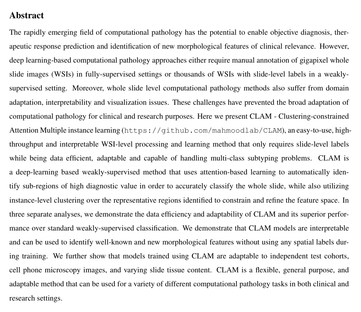
The rapidly emerging field of computational pathology has the potential to enable objective diagnosis, therapeutic response prediction and identification of new morphological features of clinical relevance. However, deep learning-based computational pathology approaches either require manual annotation of gigapixel whole slide images (WSIs) in fully-supervised settings or thousands of WSIs with slide-level labels in a weakly-supervised setting. Moreover, whole slide level computational pathology methods also suffer from domain adaptation and interpretability issues. These challenges have prevented the broad adaptation of computational pathology for clinical and research purposes. Here we present CLAM - Clustering-constrained attention multiple instance learning, an easy-to-use, high-throughput, and interpretable WSI-level processing and learning method that only requires slide-level labels while being data efficient, adaptable and capable of handling multi-class subtyping problems. CLAM is a deep-learning-based weakly-supervised method that uses attention-based learning to automatically identify sub-regions of high diagnostic value in order to accurately classify the whole slide, while also utilizing instance-level clustering over the representative regions identified to constrain and refine the feature space. In three separate analyses, we demonstrate the data efficiency and adaptability of CLAM and its superior performance over standard weakly-supervised classification. We demonstrate that CLAM models are interpretable and can be used to identify well-known and new morphological features. We further show that models trained using CLAM are adaptable to independent test cohorts, cell phone microscopy images, and biopsies. CLAM is a general-purpose and adaptable method that can be used for a variety of different computational pathology tasks in both clinical and research settings.

Topics

cell phone classification deep learning feature space general purpose high resolution image interpretability subtyping clustering methods computational efficiency

Keywords

computational pathology whole-slide images weak supervision slide-level diagnosis metastasis detection cancer subtyping attention network stain normalization

References

Knowls

Knowl 1 — Multi-Branch Attention Pooling in CLAM
model/method
Clustering-constrained Attention Multiple Instance Learning (CLAM) aggregates patch-level embeddings into slide-level representations for $n$ -class classification via class-specific attention branches.

Let a whole slide image (WSI) contain $N$ patches. Each patch $k$ ( $1 \le k \le N$ ) is first represented by a 1024-dimensional feature embedding $z_k \in \mathbb{R}^{1024}$ extracted via a pretrained convolutional neural network. A linear projection layer with weights $W_1 \in \mathbb{R}^{512 \times 1024}$ compresses $z_k$ to a 512-dimensional vector: $h_k = W_1 z_k^\top \in \mathbb{R}^{512}$

The network features an attention backbone consisting of two parameter matrices $U_a \in \mathbb{R}^{256 \times 512}$ and $V_a \in \mathbb{R}^{256 \times 512}$ , followed by $n$ parallel attention heads $W_{a,1}, \dots, W_{a,n} \in \mathbb{R}^{1 \times 256}$ . For the $m$ -th class ( $m \in \{1, \dots, n\}$ ), the attention score $a_{k,m}$ of patch $k$ is defined by gated attention pooling: $a_{k,m} = \frac{\exp\left\{ W_{a,m} \left( \tanh(V_a h_k^\top) \odot \text{sigm}(U_a h_k^\top) \right) \right\}}{\sum_{j=1}^N \exp\left\{ W_{a,m} \left( \tanh(V_a h_j^\top) \odot \text{sigm}(U_a h_j^\top) \right) \right\}}$ where $\odot$ denotes element-wise multiplication and $\text{sigm}(\cdot)$ denotes the standard sigmoid function.

The aggregated slide-level representation for class $m$ , denoted $h_{\text{slide},m} \in \mathbb{R}^{1 \times 512}$ , is the attention-weighted average: $h_{\text{slide},m} = \sum_{k=1}^N a_{k,m} h_k$

An independent linear classifier $W_{c,m} \in \mathbb{R}^{1 \times 512}$ evaluates each representation to compute the unnormalized slide score $s_{\text{slide},m} = W_{c,m} h_{\text{slide},m}^\top$ . The final probability distribution over the $n$ classes is obtained by applying the softmax function to the vector $s_{\text{slide}} = [s_{\text{slide},1}, \dots, s_{\text{slide},n}]^\top$ .
Knowl 2 — Instance-Level Clustering with Attention Pseudo-Labeling
algorithm
CLAM refines the patch-level representation space during training by generating pseudo-labels from attention scores and supervising linear clustering layers $W_{\text{inst},m} \in \mathbb{R}^{2 \times 512}$ for each class $m \in \{1, \dots, n\}$ .
function CLUSTER((h_1, a_1), ..., (h_K, a_K), Y, mutually_exclusive, B)
    Input: Patch embeddings h_k in R^{512} and attention vectors a_k in R^n for k = 1 to K; ground truth slide label Y in {1, ..., n}; boolean flag mutually_exclusive; number of samples B.
    Output: Predictions p and pseudo-labels y for clustering loss calculation.

    for m <- 1 to n do
        if m = Y then
            (h_sorted, a_sorted) <- SortAscendingByAttention((h_1, a_{1,m}), ..., (h_K, a_{K,m}))
            for b <- 1 to B do
                y_{m,b} <- 0
                y_{m,b+B} <- 1
                p_{m,b} <- W_{inst,m} (h_sorted[b])^T
                p_{m,b+B} <- W_{inst,m} (h_sorted[K - B + b])^T
        else
            if mutually_exclusive = True then
                (h_sorted, a_sorted) <- SortAscendingByAttention((h_1, a_{1,m}), ..., (h_K, a_{K,m}))
                for b <- 1 to B do
                    y_{m,b} <- 0
                    p_{m,b} <- W_{inst,m} (h_sorted[K - B + b])^T
            else
                pass

    if mutually_exclusive = True then
        return [p_1, ..., p_n], [y_1, ..., y_n]
    else
        return [p_Y], [y_Y]
For the ground-truth branch $Y$ , the $B$ patches with lowest attention are labeled negative ( $y=0$ , non-informative/background evidence) and the $B$ patches with highest attention are labeled positive ( $y=1$ , strong positive evidence). When classes are mutually exclusive (e.g., distinct cancer subtypes), the top $B$ attended patches from out-of-class branches $m \ne Y$ are assigned pseudo-label $0$ as false-positive evidence.
Knowl 3 — Smooth Top-1 Multiclass SVM Loss
equation
For the instance-level patch clustering task in CLAM, a smooth variant of the multiclass top-1 SVM loss is used instead of standard cross-entropy to increase robustness against noisy pseudo-labels.

Let $\mathcal{Y} = \{0, 1, \dots, n-1\}$ denote the set of class labels, $y \in \mathcal{Y}$ the ground truth label, and $s \in \mathbb{R}^n$ the predicted score vector. The classical hard multiclass SVM loss with margin $\alpha$ is: $l(s, y) = \max\left( \max_{j \in \mathcal{Y} \setminus \{y\}} \{s_j + \alpha\} - s_y,\; 0 \right)$

The smoothed, infinitely differentiable top-1 SVM loss $L_{1,\tau}(s, y)$ incorporates a temperature scaling parameter $\tau > 0$ : $L_{1,\tau}(s, y) = \tau \log \left[ \sum_{j \in \mathcal{Y}} \exp\left( \frac{1}{\tau} (\alpha \mathbf{1}(j \ne y) + s_j - s_y) \right) \right]$ where $\mathbf{1}(\cdot)$ is the indicator function. In CLAM instance clustering, this is evaluated as a binary loss ( $|\mathcal{Y}| = 2$ ) on the cluster predictions with hyperparameters set to $\alpha = 1.0$ and $\tau = 1.0$ .
Knowl 4 — CLAM Optimization Objective and Training Configuration
model/method
The overall loss $\mathcal{L}_{\text{total}}$ for a single whole slide image is a linear combination of the slide-level classification loss $\mathcal{L}_{\text{slide}}$ and the patch-level clustering loss $\mathcal{L}_{\text{patch}}$ : $\mathcal{L}_{\text{total}} = c_1 \mathcal{L}_{\text{slide}} + c_2 \mathcal{L}_{\text{patch}}$ where $c_1 = 0.7$ and $c_2 = 0.3$ .
- $\mathcal{L}_{\text{slide}}$ is standard cross-entropy calculated between the slide-level prediction vector $s_{\text{slide}}$ and the ground truth slide label $Y$ .
- $\mathcal{L}_{\text{patch}}$ is the binary smooth top-1 SVM loss computed over all sampled patches and their corresponding pseudo-labels generated by the attention network ( $2B$ patches for the in-class branch, and $B$ patches for each of the $n-1$ out-of-class branches under mutual exclusivity, with $B = 8$ ).
Training details:
- Batch size: 1 slide per iteration.
- Sampling strategy: Multinomial sampling probability for each slide is inversely proportional to its class frequency to correct for training set class imbalance.
- Optimizer: Adam with learning rate $2 \times 10^{-4}$ and $L_2$ weight decay of $1 \times 10^{-5}$ .
- Early stopping: Models are trained for a minimum of 50 epochs up to 200 epochs, terminating early if validation loss fails to reach a new low for 20 consecutive epochs.
Knowl 5 — WSI Processing and Feature Extraction Pipeline
model/method
CLAM processes gigapixel whole slide images through a three-stage automated pipeline:
1. Tissue Segmentation: The WSI is downsampled (e.g., $32\times$ ) and converted to the HSV color space. A foreground binary mask is obtained by thresholding the saturation channel after median blurring to remove noise and smooth boundaries, followed by morphological closing to fill small holes. Foreground object contours are filtered by area threshold.
2. Patching: Non-overlapping $256 \times 256$ pixel patches are cropped exhaustively from the segmented foreground at the specified magnification ( $20\times$ or $40\times$ ) and stored alongside slide coordinates in HDF5 format.
3. Feature Extraction: Patches are fed in batches (size 128 per GPU) into a ResNet50 convolutional neural network pretrained on ImageNet. Features are extracted via adaptive mean-spatial pooling after the 3rd residual block, converting each $256 \times 256$ patch into a 1024-dimensional feature embedding $z_k$ .
This feature extraction reduces data volume approximately 200-fold, allowing all patch embeddings for a WSI (up to 150,000+ patches) to fit simultaneously into consumer GPU memory during training.
Knowl 6 — High-Resolution Attention Heatmap Generation
model/method
CLAM generates spatial interpretability heatmaps of whole slide images without requiring pixel-level or patch-level annotations during training.
1. For a given slide, unnormalized attention scores are computed for all cropped patches using the attention branch corresponding to the model's predicted slide class.
2. Raw attention scores are converted to percentile ranks (scaled between $0.0$ and $1.0$ , where $1.0$ represents the highest attention / positive evidence and $0.0$ represents the lowest attention / negative evidence) based on the unnormalized score distribution of non-overlapping patches across the entire slide.
3. Normalized scores are mapped to RGB colors using a diverging colormap (red for high attention, blue for low attention).
4. To produce fine-grained, smooth heatmaps over regions of interest (ROIs) or entire slides, patches are cropped with a high degree of spatial overlap (e.g., $95\%$ overlap). Overlapping patch scores are evaluated, normalized against the whole-slide percentile reference, accumulated, and averaged per spatial pixel, then overlaid onto the original H&E image at a transparency of $0.5$ .
Knowl 7 — Diagnostic Classification Performance on Public Resection Datasets
empirical result
CLAM was evaluated on three diagnostic tasks using 10-fold Monte Carlo cross-validation (80% train, 10% validation, 10% test per fold) on public resection datasets:
1. Renal Cell Carcinoma (RCC) Subtyping: Evaluated on 884 diagnostic WSIs from TCGA (111 Chromophobe RCC, 489 Clear Cell RCC, 284 Papillary RCC) at $20\times$ magnification. Achieved a 10-fold macro-averaged one-vs-rest test Area Under the Curve (AUC) of $0.991 \pm 0.006$ .
2. Non-Small Cell Lung Cancer (NSCLC) Subtyping: Evaluated on 1,967 diagnostic WSIs from TCGA and CPTAC (1,175 Lung Adenocarcinoma [LUAD], 792 Lung Squamous Cell Carcinoma [LUSC]) at $20\times$ magnification. Achieved a 10-fold mean test AUC of $0.956 \pm 0.018$ .
3. Axillary Lymph Node Metastasis Detection: Evaluated on 899 WSIs from Camelyon16 and Camelyon17 (591 negative, 308 positive) at $40\times$ magnification. Achieved a 10-fold mean test AUC of $0.953 \pm 0.029$ .
Knowl 8 — Generalization to Independent Resection Test Cohorts
empirical result
Models trained on public repositories were evaluated directly without fine-tuning on independent clinical cohorts collected and scanned at Brigham and Women's Hospital (BWH):
- BWH RCC Resection Cohort ( $n=135$ slides; 43 CRCC, 46 CCRCC, 46 PRCC): The 10-fold cross-validated models trained on TCGA achieved a macro-averaged one-vs-rest test AUC of $0.973 \pm 0.006$ . Ensembling all 10 models achieved a macro-averaged AUC of $0.980$ (95% CI: $0.936$ – $1.000$ for CRCC, $0.979$ – $1.000$ for CCRCC, $0.951$ – $1.000$ for PRCC).
- BWH NSCLC Resection Cohort ( $n=131$ slides; 63 LUAD, 68 LUSC): Models trained on TCGA+CPTAC achieved an average test AUC of $0.975 \pm 0.007$ . The 10-model ensemble achieved an AUC of $0.980$ (95% CI: $0.954$ – $1.000$ ).
- BWH Axillary Lymph Node Cohort ( $n=133$ slides; 66 negative, 67 positive): Models trained on Camelyon16/17 achieved an average test AUC of $0.934 \pm 0.018$ . The 10-model ensemble achieved an AUC of $0.945$ (95% CI: $0.907$ – $0.984$ ).
Knowl 9 — Adaptability to Biopsy WSIs and Cellphone Microscopy Images
empirical result
CLAM models trained exclusively on resection WSIs were directly evaluated without fine-tuning on core needle biopsy slides and consumer cellphone microscopy images (CPIs) from BWH:
- Biopsy WSIs:
  - NSCLC Biopsy ( $n=110$ slides; 55 LUAD, 55 LUSC): Mean test AUC of $0.902 \pm 0.016$ (best single model: $0.926$ ; ensemble AUC: $0.923$ , 95% CI: $0.874$ – $0.973$ ).
  - RCC Biopsy ( $n=92$ slides; 53 CCRCC, 26 PRCC, 13 CRCC): Mean macro-averaged test AUC of $0.951 \pm 0.011$ (best single model: $0.967$ ; ensemble macro AUC: $0.960$ ).
- Cellphone Microscopy Images (CPIs) (4–8 representative fields-of-view captured at $20\times$ per slide):
  - NSCLC CPIs ( $n=131$ cases): Mean test AUC of $0.873 \pm 0.025$ (best single model: $0.899$ ; ensemble AUC: $0.883$ , 95% CI: $0.824$ – $0.941$ ). Drop of $0.102$ in mean AUC relative to scanned resection WSIs.
  - RCC CPIs ( $n=135$ cases): Mean macro-averaged test AUC of $0.921 \pm 0.023$ (best single model: $0.958$ ; ensemble macro AUC: $0.943$ ). Drop of $0.051$ in mean AUC relative to scanned resection WSIs.
Knowl 10 — Data Efficiency and Superiority Over Standard Max-Pooling Multiple Instance Learning
empirical result
CLAM was evaluated across subsampled training set sizes (100%, 75%, 50%, 25%, and 10% of total cases) and compared directly against standard max-pooling multiple instance learning (MIL for binary, mMIL for multiclass):
- Data Efficiency: For RCC subtyping, training on 25% of cases (~170 slides per fold) yielded a test AUC of $>0.94$ ( $0.946 \pm 0.017$ ). For NSCLC subtyping and lymph node metastasis detection, training on 50% of cases (~853 and ~289 slides, respectively) maintained test AUCs of $0.937 \pm 0.022$ and $0.921 \pm 0.032$ .
- Comparison with MIL / mMIL:
  - CLAM outperformed max-pooling MIL/mMIL across nearly all training set sizes and tasks.
  - In low-data regimes (25% training data), CLAM outperformed mMIL/MIL on the independent BWH test cohort by an average of $+14.5\%$ in test AUC for RCC subtyping and $+30.1\%$ in test AUC for lymph node metastasis detection.
  - For NSCLC subtyping, CLAM outperformed MIL by $3\%$ to $5\%$ in test AUC across most dataset sizes.
  - Standard max-pooling MIL showed extreme sensitivity to data splits and stochastic initialization in lymph node metastasis detection, frequently failing to converge (AUC near $0.5$ ) when trained on small subsets (10% and 25%), whereas CLAM converged reliably.

Coverage note — None was omitted; the full methodology, mathematical formulation, training protocol, preprocessing pipeline, and primary empirical evaluations across all tasks and modalities are covered.

References

1.Bera, K., Schalper & Madabhushi, A. Artificial intelligence in digital pathologynew tools for diagnosis and precision oncology. Nature Reviews Clinical Oncology 16, 703–715 (2019).
2.Niazi, M. K. K., Parwani, A. V. & Gurcan, M. N. Digital pathology and artificial intelligence. The Lancet Oncology 20, e253–e261 (2019).
3.Hollon, T. C. et al. Near real-time intraoperative brain tumor diagnosis using stimulated raman histology and deep neural networks. Nature Medicine 1–7 (2020).
4.Kather, J. N. et al. Deep learning can predict microsatellite instability directly from histology in gastrointestinal cancer. Nature medicine 25, 1054–1056 (2019).
5.Bulten, W. et al. Automated deep-learning system for gleason grading of prostate cancer using biopsies: a diagnostic study. The Lancet Oncology (2020).
6.Ström, P. et al. Artificial intelligence for diagnosis and grading of prostate cancer in biopsies: a population-based, diagnostic study. The Lancet Oncology (2020).
7.Schapiro, D. et al. histocat: analysis of cell phenotypes and interactions in multiplex image cytometry data. Nature methods 14, 873 (2017).
8.Moen, E. et al. Deep learning for cellular image analysis. Nature methods 1–14 (2019).
9.Mahmood, F. et al. Deep adversarial training for multi-organ nuclei segmentation in histopathology images. IEEE transactions on medical imaging (2019).
10.Graham, S. et al. Hover-net: Simultaneous segmentation and classification of nuclei in multi-tissue histology images. Medical Image Analysis 58, 101563 (2019).
11.Saltz, J. et al. Spatial organization and molecular correlation of tumor-infiltrating lymphocytes using deep learning on pathology images. Cell reports 23, 181–193 (2018).
12.Javed, S. et al. Cellular community detection for tissue phenotyping in colorectal cancer histology images. Medical Image Analysis 101696 (2020).
13.Mobadersany, P. et al. Predicting cancer outcomes from histology and genomics using convolutional networks. Proceedings of the National Academy of Sciences 115, E2970–E2979 (2018).
14.Heindl, A. et al. Microenvironmental niche divergence shapes brca1-dysregulated ovarian cancer morphological plasticity. Nature communications 9, 1–14 (2018).
15.Yuan, Y. et al. Quantitative image analysis of cellular heterogeneity in breast tumors complements genomic profiling. Science translational medicine 4, 157ra143–157ra143 (2012).
16.Lazar, A. J. et al. Comprehensive and integrated genomic characterization of adult soft tissue sarcomas. Cell 171, 950–965 (2017).
17.Beck, A. H. et al. Systematic analysis of breast cancer morphology uncovers stromal features associated with survival. Science translational medicine 3, 108ra113–108ra113 (2011).
18.Yamamoto, Y. et al. Automated acquisition of explainable knowledge from unannotated histopathology images. Nature Communications 10, 1–9 (2019).
19.Pell, R. et al. The use of digital pathology and image analysis in clinical trials. The Journal of Pathology: Clinical Research 5, 81–90 (2019).
20.LeCun, Y., Bengio, Y. & Hinton, G. Deep learning. nature 521, 436–444 (2015).
21.Esteva, A. et al. A guide to deep learning in healthcare. Nature medicine 25, 24–29 (2019).
22.Esteva, A. et al. Dermatologist-level classification of skin cancer with deep neural networks. Nature 542, 115–118 (2017).
23.Poplin, R. et al. Prediction of cardiovascular risk factors from retinal fundus photographs via deep learning. Nature Biomedical Engineering 2, 158 (2018).
24.McKinney, S. M. et al. International evaluation of an ai system for breast cancer screening. Nature 577, 89–94 (2020).
25.Mitani, A. et al. Detection of anaemia from retinal fundus images via deep learning. Nature Biomedical Engineering 4, 18–27 (2020).
26.Shen, L., Zhao, W. & Xing, L. Patient-specific reconstruction of volumetric computed tomography images from a single projection view via deep learning. Nature biomedical engineering 3, 880–888 (2019).
27.Bejnordi, B. E. et al. Diagnostic assessment of deep learning algorithms for detection of lymph node metastases in women with breast cancer. Jama 318, 2199–2210 (2017).
28.Chen, P.-H. C. et al. An augmented reality microscope with real-time artificial intelligence integration for cancer diagnosis. Nature medicine 25, 1453–1457 (2019).
29.Nagpal, K. et al. Development and validation of a deep learning algorithm for improving gleason scoring of prostate cancer. NPJ digital medicine 2, 1–10 (2019).
30.Coudray, N. et al. Classification and mutation prediction from non–small cell lung cancer histopathology images using deep learning. Nature medicine 24, 1559–1567 (2018).
31.Campanella, G. et al. Clinical-grade computational pathology using weakly supervised deep learning on whole slide images. Nature medicine 25, 1301–1309 (2019).
32.Maron, O. & Lozano-Pérez, T. A framework for multiple-instance learning. In Advances in neural information processing systems, 570–576 (1998).
33.Ilse, M., Tomczak, J. & Welling, M. Attention-based deep multiple instance learning. In International Conference on Machine Learning, 2132–2141 (2018).
34.BenTaieb, A. & Hamarneh, G. Adversarial stain transfer for histopathology image analysis. IEEE transactions on medical imaging 37, 792–802 (2017).
35.Couture, H. D., Marron, J. S., Perou, C. M., Troester, M. A. & Niethammer, M. Multiple instance learning for heterogeneous images: Training a cnn for histopathology. In International Conference on Medical Image Computing and Computer-Assisted Intervention, 254–262 (Springer, 2018).
36.Kraus, O. Z., Ba, J. L. & Frey, B. J. Classifying and segmenting microscopy images with deep multiple instance learning. Bioinformatics 32, i52–i59 (2016).
37.Zhang, C., Platt, J. C. & Viola, P. A. Multiple instance boosting for object detection. In Advances in neural information processing systems, 1417–1424 (2006).
38.Berrada, L., Zisserman, A. & Kumar, M. P. Smooth loss functions for deep top-k classification. In International Conference on Learning Representations (2018).
39.Crammer, K. & Singer, Y. On the algorithmic implementation of multiclass kernel-based vector machines. Journal of machine learning research 2, 265–292 (2001).
40.Litjens, G. et al. 1399 h&e-stained sentinel lymph node sections of breast cancer patients: the camelyon dataset. GigaScience 7, giy065 (2018).

Citation

MLA

Lu, M. Y., et al. “Data Efficient and Weakly Supervised Computational Pathology on Whole Slide Images”. arXiv, 2020, http://arxiv.org/abs/2004.09666v2.

APA

Lu, M. Y., Williamson, D. F. K., Chen, T. Y., Chen, R. J., Barbieri, M., & Mahmood, F. (2020). Data Efficient and Weakly Supervised Computational Pathology on Whole Slide Images. arXiv. http://arxiv.org/abs/2004.09666v2

Chicago

Lu, M. Y., D. F. K. Williamson, T. Y. Chen, R. J. Chen, M. Barbieri, and F. Mahmood. 2020. “Data Efficient and Weakly Supervised Computational Pathology on Whole Slide Images”. arXiv. http://arxiv.org/abs/2004.09666v2.

Harvard

Lu, M.Y. et al. (2020) “Data Efficient and Weakly Supervised Computational Pathology on Whole Slide Images”, arXiv [Preprint]. Available at: http://arxiv.org/abs/2004.09666v2.

Vancouver

1. Lu MY, Williamson DFK, Chen TY, Chen RJ, Barbieri M, Mahmood F (2020) Data Efficient and Weakly Supervised Computational Pathology on Whole Slide Images. arXiv

BibTeX

@article{lu2020data,
  title = {Data Efficient and Weakly Supervised Computational Pathology on Whole Slide Images},
  author = {Lu, Ming Y. and Williamson, Drew F. K. and Chen, Tiffany Y. and Chen, Richard J. and Barbieri, Matteo and Mahmood, Faisal},
  year = {2020},
  journal = {arXiv},
  url = {http://arxiv.org/abs/2004.09666v2},
  eprint = {2004.09666}
}

Metadata:arXiv

Source Code

This paper has an official code repository available. Click below to access the source code.

View Repository

Access the Paper

This paper is available from its original source. Click below to access the PDF.

Open PDF

Data-efficient and weakly supervised computational pathology on whole-slide images

Abstract

Topics

Keywords

Table of Contents

Knowls

Knowl 1 — Multi-Branch Attention Pooling in CLAM

Knowl 2 — Instance-Level Clustering with Attention Pseudo-Labeling

Knowl 3 — Smooth Top-1 Multiclass SVM Loss

Knowl 4 — CLAM Optimization Objective and Training Configuration

Knowl 5 — WSI Processing and Feature Extraction Pipeline

Knowl 6 — High-Resolution Attention Heatmap Generation

Knowl 7 — Diagnostic Classification Performance on Public Resection Datasets

Knowl 8 — Generalization to Independent Resection Test Cohorts

Knowl 9 — Adaptability to Biopsy WSIs and Cellphone Microscopy Images

Knowl 10 — Data Efficiency and Superiority Over Standard Max-Pooling Multiple Instance Learning

References

Citation

BibTeX

Source Code

Access the Paper