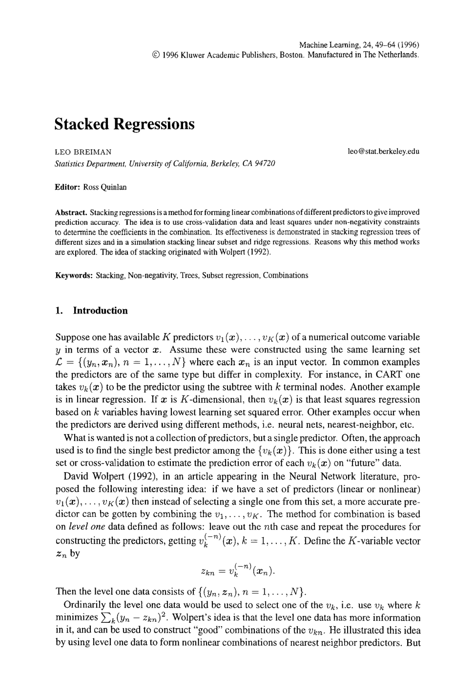
Stacked regressions

LEO BREIMAN

article2004Machine-mediated learning1,413 citations

Demonstrates how combining multiple regression models using cross-validation under non-negativity constraints reliably outperforms single-model selection across diverse algorithms like decision trees, subset selection, and ridge regression.

Listen

In predictive modeling, practitioners traditionally evaluate a range of competing models and select the single best performer using holdout validation or cross-validation. However, choosing only one model discards valuable information present in alternative predictors and risks poor generalization when models are sensitive to sample variations. The article addresses this limitation by developing stacked regressions, a method for forming linear combinations of different predictors to achieve superior prediction accuracy compared to any individual model.

The article establishes and evaluates a practical framework that uses cross-validated predictions paired with least squares estimation constrained by non-negative weights to determine the combination coefficients. The approach was tested across real-world datasets and extensive computer simulations. Specifically, the analysis evaluated decision trees using the Boston Housing and Ozone datasets, alongside 250 simulation runs involving 40 variables and 60 observations across varied correlation structures to test subset regressions, ridge regressions, and their combinations.

The findings show that stacked regressions consistently outperform the single best model chosen by cross-validation. On the real-world housing and ozone datasets, stacking regression trees reduced prediction error by approximately 10%. In linear simulations, stacking subset regressions and ridge regressions together delivered substantial reductions in model error, outperforming the best-of-best single model selection across all evaluated scenarios. Additionally, the analysis revealed that only a small number of predictors receive positive weights—typically around 3 to 7 models out of dozens—and that 10-fold cross-validation is not only computationally faster than leave-one-out cross-validation but also yields slightly better predictive accuracy.

These results demonstrate that combining diverse predictive models provides greater accuracy and stability than relying on a single selected model. The greatest performance gains occur when combining dissimilar model types, such as subset selection with regularized models, because differing models capture complementary patterns in data. In organizational settings, shifting from single-model selection to stacked combinations can improve decision performance and mitigate model-selection risk without requiring unconstrained, complex combinations that risk overfitting.

Organizations and practitioners should adopt stacked regression with non-negativity constraints when selecting among diverse model candidates. For implementation efficiency, teams should use 10-fold cross-validation rather than leave-one-out methods. While the empirical and simulation evidence strongly supports the method, the article notes that general mathematical proofs are not yet complete, and stacking yields minimal gains when combining highly similar models. Additional evaluation is warranted when applying the approach to other model families such as neural networks or spline-based models.

University of California Berkeley cross validation non-negativity regression model stacked regressions subset regression ridge regression

BREIMAN (2004).pdf

Paper: Bagging Predictors, Leo Breiman (1996). Introduces bootstrap aggregation (bagging) to reduce predictor variance, providing essential foundational context for ensemble model combination methods.
Paper: Regression Shrinkage and Selection Via the Lasso, Robert Tibshirani (1996). Establishes constrained regularized regression techniques that underly the non-negativity and shrinkage constraints used when combining predictors in stacked regressions.
Paper: A Study of Cross-Validation and Bootstrap for Accuracy Estimation and Model Selection, Ron Kohavi (1995). Provides a comprehensive analysis of cross-validation methodology, which is the core mechanism used in stacked regressions to form out-of-fold predictions and prevent overfitting.
Paper: Greedy function approximation: A gradient boosting machine, Jerome H. Friedman (2001). Presents gradient boosting as an alternative framework for ensembling decision trees and regression models through stagewise optimization.
Paper: Random Forests, Leo Breiman (2001). Details the random forest paradigm for aggregating randomized regression and classification trees, contrasting simple averaging with meta-learning combinations.

Paper: FFORMA: Feature-based forecast model averaging, Pablo Montero-Manso et al. (2020). Extends meta-learning and model combination principles from stacked regressions to time-series forecasting via feature-based forecast model averaging.
Paper: An empirical comparison of supervised learning algorithms, Rich Caruana et al. (2006). Evaluates a wide spectrum of modern supervised algorithms and ensemble architectures across varied metrics and probability calibration methods.
Paper: Rotation Forest: A New Classifier Ensemble Method, Juan J. Rodríguez et al. (2006). Explores feature-space rotation to induce model diversity, offering an alternative pathway for constructing complementary base predictors for ensemble learning.
Paper: BART: Bayesian Additive Regression Trees, Hugh A. Chipman et al. (2008). Develops a Bayesian ensemble framework that regularizes sum-of-trees models to provide full posterior inference and uncertainty quantification.
Paper: Model soups: averaging weights of multiple fine-tuned models improves accuracy without increasing inference time, Mitchell Wortsman et al. (2022). Applies model combination principles to modern neural architectures by averaging model weights directly to gain ensemble-like benefits without test-time overhead.

Abstract

Stacking regressions is a method for forming linear combinations of different predictors to give improved prediction accuracy. The idea is to use cross-validation data and least squares under non-negativity constraints to determine the coefficients in the combination. Its effectiveness is demonstrated in stacking regression trees of different sizes and in a simulation stacking linear subset and ridge regressions. Reasons why this method works are explored. The idea of stacking originated with Wolpert (1992).

Topics

cross validation non-negativity regression model validation multiple regression random forests

Keywords

stacked regressions subset regression ridge regression regression trees linear regression subset selection non-negativity constraints cross-validation prediction

1. Introduction
2. Why Non-negativity Constraints Work
3. Stacking Trees
4. Description of the Linear Regression Simulation
5. Stacking Subset Regressions
6. Stacking Ridge Regression
7. Stacking Subset Selection With Ridge
8. Computational Efficiency and J-Fold Cross-Validation
9. Remarks
10. Conclusions
References

Knowls

Knowl 1 — Stacked Regression with Non-Negative Least Squares
model/method
Stacked regression combines $K$ predictors $v_1(x), \ldots, v_K(x)$ of a continuous response $y \in \mathbb{R}$ from an input vector $x \in \mathbb{R}^M$ , constructed from a training dataset $\mathcal{L} = \{(y_n, x_n)\}_{n=1}^N$ . To avoid overfitting and collinearity instabilities inherent in unconstrained least squares combinations, stacking uses cross-validation predictions (level-one data) subject to non-negativity constraints.

The training data $\mathcal{L}$ is split into $J$ folds $\mathcal{L}_1, \ldots, \mathcal{L}_J$ . For each fold $j \in \{1, \ldots, J\}$ , base predictors $v_k^{(j)}(x)$ are trained on the out-of-fold data $\mathcal{L}^{(-j)} = \mathcal{L} \setminus \mathcal{L}_j$ . For each sample $(y_n, x_n) \in \mathcal{L}_j$ , the level-one feature vector $z_n = (z_{1n}, \ldots, z_{Kn})^T$ is constructed with: $z_{kn} = v_k^{(j)}(x_n)$ When $J = N$ , this corresponds to leave-one-out cross-validation: $z_{kn} = v_k^{(-n)}(x_n)$ .

The stacking combination coefficients $\alpha = (\alpha_1, \ldots, \alpha_K)^T$ are determined by solving the non-negative least squares problem over the level-one data: $\min_{\alpha_1, \ldots, \alpha_K} \sum_{n=1}^N \left( y_n - \sum_{k=1}^K \alpha_k z_{kn} \right)^2 \quad \text{subject to} \quad \alpha_k \ge 0 \quad \text{for } k = 1, \ldots, K$

The final stacked predictor evaluated on any new input vector $x$ is: $v(x) = \sum_{k=1}^K \alpha_k v_k(x)$ where each $v_k(x)$ is the predictor trained on the full training set $\mathcal{L}$ .
Knowl 2 — Condition for Single Predictor Optimality over Stacking
theoretical result
Let $R$ be the $K \times K$ residual cross-product matrix among $K$ predictors $v_1, \ldots, v_K$ on response data $y$ , with elements: $R_{ij} = \sum_{n=1}^N (y_n - v_i(x_n))(y_n - v_j(x_n))$ Suppose combination coefficients $\alpha = (\alpha_1, \ldots, \alpha_K)^T$ are chosen to minimize $\alpha^T R \alpha$ subject to non-negativity ( $\alpha_k \ge 0$ ) and the convex combination constraint ( $\sum_{k=1}^K \alpha_k = 1$ ). Let $v_k$ be the single predictor with minimal residual sum of squares, such that $R_{kk} = \min_{j} R_{jj}$ .

The best single predictor $v_k$ is identical to the optimal stacked combination if and only if: $R_{kk} \le R_{ik} \quad \text{for all } i = 1, \ldots, K$

Equivalently, letting $\rho_{ik}$ denote the sample correlation between the residual vectors of predictor $i$ and predictor $k$ , and letting $\sigma_i, \sigma_k$ denote their respective residual standard deviations, this condition is: $\frac{\sigma_k}{\sigma_i} \le \rho_{ik} \quad \text{for all } i = 1, \ldots, K$

Consequently, if an alternative candidate predictor $v_i$ achieves residual error comparable to $v_k$ (i.e., $\sigma_i \approx \sigma_k$ ), the best single predictor cannot outperform or match stacking unless its residuals are almost perfectly correlated with $v_k$ ( $\rho_{ik} \approx 1$ ), implying that $v_i(x) \approx v_k(x)$ .
Knowl 3 — Implicit Sum-to-One Property of Non-Negative Stacking Weights
theoretical result
In stacked regression with non-negativity constraints $\alpha_k \ge 0$ , an explicit sum-to-one constraint $\sum_{k=1}^K \alpha_k = 1$ is mathematically and empirically unnecessary when accurate base predictors are present.

Let $\alpha = (\alpha_1, \ldots, \alpha_K)^T$ be the unconstrained non-negative minimizer of $\sum_{n=1}^N (y_n - \sum_k \alpha_k v_k(x_n))^2$ , let $s = \sum_{k=1}^K \alpha_k$ , and define the normalized combination predictor $v^*(x) = \sum_{k=1}^K (\alpha_k / s) v_k(x)$ and unnormalized predictor $v(x) = s v^*(x) = \sum_{k=1}^K \alpha_k v_k(x)$ . Using the sample Euclidean norm $\|u\| = \sqrt{\sum_{n=1}^N u_n^2}$ , the sum of weights $s$ satisfies: $\frac{\|y\| - \|y - v\|}{\|y\| + \|y - v^*\|} \le s \le \frac{\|y\| + \|y - v\|}{\|y\| - \|y - v^*\|}$

When at least one base predictor in the ensemble fits the target reasonably well, the residual norms $\|y - v\|$ and $\|y - v^*\|$ are small relative to the response norm $\|y\|$ , confining $s$ to a narrow neighborhood around 1.0 without enforcing $\sum_k \alpha_k = 1$ during optimization.
Knowl 4 — Equivalent Single-Tree Representation of Stacked Nested Trees
theoretical result
When CART pruning produces a nested sequence of subtrees $T_1 \subset T_2 \subset \dots \subset T_K$ (where $T_k$ denotes the pruned subtree with $k$ terminal nodes), stacking these subtrees with non-negative weights $\alpha_k \ge 0$ yields a predictor $v(x) = \sum_{k=1}^K \alpha_k v_k(x)$ that is mathematically equivalent to a single regression tree having the structure and terminal node partition of the largest tree $T_m$ in the stack ( $m = \max \{k : \alpha_k > 0\}$ ).

For any terminal node $t$ in the largest tree $T_m$ , the predicted response value $y(t)$ in the combined tree is given by: $y(t) = \sum_{k=1}^m \alpha_k \bar{y}(t_k)$ where $t_k$ is the unique ancestor node of $t$ in subtree $T_k$ , and $\bar{y}(t_k)$ is the sample mean of the target values $y$ belonging to node $t_k$ .

Stacking nested regression trees therefore acts as hierarchical shrinkage: the prediction in each terminal node of the fine tree gathers statistical strength by blending its local average with the broader sample means of its ancestor nodes in simpler subtrees.

Knowl 5 — Test Error Reduction by Stacking CART Subtrees on Real Datasets

data/table

Stacking regression trees of different terminal node sizes was evaluated on the Boston Housing dataset (506 cases, 12 variables) and the Ozone dataset (330 complete cases, 8 variables). In each of 100 iterations, 50 cases were randomly held out as test data $\mathcal{L}_{TS}$ , while 10-fold cross-validation ( $J = 10$ ) on the remaining cases was used to compute non-negative stacking weights $\alpha_k$ across approximately 50 subtrees.

	Boston Housing		Ozone
Metric	Best Single Tree	Stacked Trees	Best Single Tree	Stacked Trees
Mean Test Prediction Error	20.9	19.0	23.9	21.6
Average $\|\sum_k \alpha_k - 1\|$	—	0.04	—	0.03
Average # Subtrees in Stack	1	6.5	1	6.3

Stacking achieves an approximately 10% reduction in mean squared prediction error compared to selecting the single best cross-validated tree on both datasets. The non-negative least squares solver assigns non-zero weights to only a sparse subset (averaging 6.3 to 6.5 subtrees) out of the roughly 50 available candidate subtrees, and the unconstrained sum of weights remains within 3% to 4% of 1.0.

Knowl 6 — Synthetic Evaluation Framework for Linear Model Error
experimental setup
A standard simulation design evaluates stacked linear regressions with $N = 60$ observations and $M = 40$ predictor variables generated from a zero-mean multivariate normal distribution $\mathcal{N}(0, \Gamma)$ . The covariance matrix $\Gamma$ has elements: $\Gamma_{km} = R^{|k-m|}, \quad k, m \in \{1, \ldots, 40\}$ with correlation parameters $R \in \{0.7, 0, -0.7\}$ .

The response variable is generated as $Y = \sum_{m=1}^{40} \beta_m X_m + \epsilon$ , where $\epsilon \sim \mathcal{N}(0, 1)$ . The true regression coefficients $\beta_m = \gamma \alpha_m$ are structured into three clusters centered at indices $m \in \{10, 20, 30\}$ parameterized by an integer width $h \in \{1, 2, 3, 4, 5\}$ : $\alpha_m = (h - |m - c|)^2 \quad \text{if } |m - c| < h \text{ for } c \in \{10, 20, 30\}, \quad \text{and } \alpha_m = 0 \text{ otherwise}$ Setting $h = 1$ yields 3 strong non-zero coefficients; setting $h = 5$ yields 27 weak non-zero coefficients. The constant $\gamma$ is calibrated in each setting such that the theoretical signal-to-noise ratio satisfies: $R^2 = \frac{\mathbb{E}\left[\left(\sum_{m=1}^{40} \beta_m X_m\right)^2\right]}{1 + \mathbb{E}\left[\left(\sum_{m=1}^{40} \beta_m X_m\right)^2\right]} = 0.5$

Performance across 250 independent replications is evaluated by the scaled Model Error (ME): $N \cdot \text{ME} = N (\hat{\beta} - \beta)^T \Gamma (\hat{\beta} - \beta)$
Knowl 7 — Performance of Stacked Stepwise Subset Regressions
empirical result
In synthetic linear regression simulations with $N=60$ cases and $M=40$ predictors across correlation settings $R \in \{0.7, 0, -0.7\}$ and coefficient patterns $h \in \{1, 2, 3, 4, 5\}$ , stacking the 40 linear models generated by backward stepwise variable deletion via non-negative least squares uniformly outperforms selecting the single best subset model via cross-validation.

The scaled model error $N \cdot \text{ME}$ of the stacked subset regression is consistently lower across all 15 simulation configurations, with estimated standard errors ranging from 0.7 to 1.0 for stacked regression compared to 1.3 to 2.0 for the cross-validation selected best subset model.

Stacking also uniformly outperforms three heuristic model mixtures:
1. An equally weighted mixture of the 5 subsets with lowest cross-validation error.
2. An equally weighted mixture of the 10 subsets with lowest cross-validation error.
3. An adaptive mixture of all models with estimated cross-validation error within $\widehat{\text{PE}}_{\min} + 0.2(\widehat{\text{PE}}_{\text{full}} - \widehat{\text{PE}}_{\min})$ (or $0.4$ if fewer than four models qualify).
Across all 15 simulation configurations, the average number of subset models assigned non-zero stacking weights $\alpha_k > 0$ is 3.1 (ranging between 2.9 and 3.4).
Knowl 8 — Joint Stacking of Stepwise Subset and Ridge Regressions
empirical result
Stacking was evaluated on a combined ensemble containing both $K = 40$ stepwise backward deletion subset models and $K' = 40$ ridge regression models corresponding to regularization parameters $\lambda_k = 0.1 k^2$ ( $k = 1, \ldots, 40$ ), forming an 80-dimensional non-negative least squares problem on cross-validation level-one data.

This joint stack was compared against a "best of best" baseline that selects the single best subset regression by cross-validation and the single best ridge regression by cross-validation, and then selects whichever of the two has lower estimated prediction error.

Across all combinations of predictor correlation $R \in \{0.7, 0, -0.7\}$ and coefficient structure $h \in \{1, 2, 3, 4, 5\}$ , joint stacking achieves uniformly lower model error than the "best of best" selector, often by large margins. The estimated standard errors of $N \cdot \text{ME}$ are 0.6 to 0.9 for joint stacking versus 0.7 to 2.1 for "best of best". The average number of non-zero model weights in the combined stack is 3.4 (ranging from 2.9 to 3.6).
Knowl 9 — Predictor Diversity and the Differential Gain of Stacking Ridge versus Subset Regressions
empirical result
Stacking ridge regressions across different penalty parameters $\lambda_1, \ldots, \lambda_K$ achieves substantial reductions in model error over the single best CV-selected ridge model only when predictor variables exhibit negative correlation ( $R = -0.7$ ), with minimal to no gain at $R = 0$ or $R = 0.7$ . In contrast, stacking subset regressions produces large and consistent reductions across all correlation structures.

This difference arises because stepwise subset regression causes sharp, discrete changes in coefficient estimates when transitioning from $k+1$ to $k$ variables, producing diverse candidate predictors. Ridge regression modifies coefficients smoothly and continuously as $\lambda$ varies from $\lambda_k$ to $\lambda_{k+1}$ , meaning candidate models close to the optimal ridge parameter are highly collinear and provide little complementary predictive value.

In simulations, stacked ridge retains an average of only 1.6 to 2.3 active models with non-zero weights, compared to 2.9 to 3.4 for subset stacking. Stacking delivers its greatest accuracy gains when the combined base predictors are structurally dissimilar.

Knowl 10 — Comparison of 10-Fold Cross-Validation and Leave-One-Out for Level-One Data

data/table

Level-one training data generated by 10-fold cross-validation ( $J=10$ ) was compared against leave-one-out cross-validation ( $J=N=60$ ) across 250 simulation iterations for three predictor correlation settings ( $R \in \{-0.7, 0, 0.7\}$ ) with $N=60$ and $M=40$ .

Method	$R = -0.7$	$R = 0$	$R = 0.7$
Best Subset	45.6 [43.5]	43.9 [42.7]	35.3 [33.8]
Best Ridge	43.3 [43.5]	34.5 [34.5]	17.1 [17.3]
Best of Best	44.3 [41.3]	36.0 [32.8]	21.3 [19.2]
Stacked Subsets	34.2 [32.7]	33.6 [31.4]	28.7 [27.9]
Stacked Ridge-Subset	33.5 [32.3]	31.2 [29.0]	19.8 [18.0]

Entries report average scaled Model Error ( $N \cdot \text{ME}$ ); the unbracketed value denotes leave-one-out cross-validation and the bracketed value denotes 10-fold cross-validation. In addition to being substantially less computationally demanding, 10-fold cross-validation achieves slightly lower model error than leave-one-out cross-validation across nearly every selection and stacking strategy.

Coverage note — Brief exploratory mentions of stacking linear regressions with k-nearest neighbors and preliminary unconstrained vs constrained numerical runs in Table 4 were omitted as they are minor extensions of the main tree and linear regression stacking results.

References

1.Belsley, D.A., Kuh, E. and Welsch, R., "Regression Diagnostics," 1980, John Wiley and Sons, New York.
2.Berger, J.O. and Bock, M.E., "Combining independent normal mean estimation problems with unknown variances," Ann. Statist. 4, 1976, pp. 642-648.
3.Breiman, L., Friedman, J., Olshen, R. and Stone, J., "Classification and Regression Trees," 1984, Wadsworth, California.
4.Breiman, L. and Friedman, J.H., "Estimating Optimal Transformations in Multiple Regression and Correlation (with discussion)," J. Amer. Statist. Assoc., 80, 1985, pp. 580-619.
5.Breiman, L. and Spector, P., "Submodel Selection and Evaluation - X Random Case," International Statistical Review, 3, 1992, pp. 291-319.
6.Efron, B. and Morris, C., "Combining possibly related estimation problems (with discussion)," J. Roy. Statist. Soc. Ser. B, 35, 1973, pp. 379-421.
7.Green, E.J. and Strawderman, W.E., "A James-Stein type estimator for combining unbiased and possibly biased estimators," J. Amer. Statist. Assoc., 86, 1991, pp. 1001-1006.
8.Hoerl, A.E. and Kennard, R.W., "Ridge regression: Biased estimation for nonorthogonal problems," Technometrics, 12, 1970, pp. 55-67.
9.Lawson, J. and Hanson, R., "Solving Least Squares Problems," 1974, Prentice-Hall, New Jersey.
10.Luenberger, D., "Linear and Nonlinear Programming," 1984, Addison-Wesley Publishing Co.
11.Le Blanc, M. and Tibshirani, R., "Combining Estimates in Regression and Classification," Technical Report 9318, 1973, Dept. of Statistics, University of Toronto.
12.Perrone, M.P., "General Averaging Results for Convex Optimization," Proceedings of the 1993 Connectionist Models Summer School, Erlbaum Associates, 1994, pp. 364-371.
13.Rao, J.N.K. and Subrahmaniam, K., "Combining independent estimators and estimation in linear regression with unequal variances," Biometrics, 27, 1971, pp. 971-990.
14.Rubin, D.B. and Weisberg, S., "The variance of a linear combination of independent estimators using estimated weights," Biometrika, 62, 1975, pp. 708-709.
15.Wolpert, D., "Stacked Generalization," Neural Networks, Vol. 5, 1992, pp. 241-259.

Citation

MLA

Breiman, L. “Stacked Regressions”. Machine Learning, vol. 24, no. 1, 1996, pp. 49–64, https://doi.org/10.1007/BF00117832.

APA

Breiman, L. (1996). Stacked regressions. Machine Learning, 24(1), 49–64. https://doi.org/10.1007/BF00117832

Chicago

Breiman, L. 1996. “Stacked Regressions”. Machine Learning 24 (1): 49–64. https://doi.org/10.1007/BF00117832.

Harvard

Breiman, L. (1996) “Stacked regressions”, Machine Learning, 24(1), pp. 49–64. Available at: https://doi.org/10.1007/BF00117832.

Vancouver

1. Breiman L (1996) Stacked regressions. Machine Learning 24:49–64

BibTeX

@article{Breiman_1996, title={Stacked regressions}, volume={24}, ISSN={1573-0565}, url={http://dx.doi.org/10.1007/BF00117832}, DOI={10.1007/bf00117832}, number={1}, journal={Machine Learning}, publisher={Springer Science and Business Media LLC}, author={Breiman, Leo}, year={1996}, month=July, pages={49–64} }

Metadata:Crossref

Access the Paper

This paper is available from its original source. Click below to access the PDF.

Open PDF

Stacked regressions

Abstract

Topics

Keywords

Table of Contents

Knowls

Knowl 1 — Stacked Regression with Non-Negative Least Squares

Knowl 2 — Condition for Single Predictor Optimality over Stacking

Knowl 3 — Implicit Sum-to-One Property of Non-Negative Stacking Weights

Knowl 4 — Equivalent Single-Tree Representation of Stacked Nested Trees

Knowl 5 — Test Error Reduction by Stacking CART Subtrees on Real Datasets

Knowl 6 — Synthetic Evaluation Framework for Linear Model Error

Knowl 7 — Performance of Stacked Stepwise Subset Regressions

Knowl 8 — Joint Stacking of Stepwise Subset and Ridge Regressions

Knowl 9 — Predictor Diversity and the Differential Gain of Stacking Ridge versus Subset Regressions

Knowl 10 — Comparison of 10-Fold Cross-Validation and Leave-One-Out for Level-One Data

References

Citation

BibTeX

Access the Paper