On Mixup Regularization

Luigi CarratinoMoustapha CisséRodolphe JenattonJean-Philippe Vert

article2022JMLR137 citations

Explains the theoretical mechanisms behind Mixup by formalizing it as empirical risk minimization with data transformation and random perturbations, leading to a simple test-time adjustment that improves prediction accuracy and calibration.

Listen

Deep neural networks are prone to overfitting and overconfident predictions, which poses risks when deploying machine learning systems in high-stakes environments. A popular data augmentation method known as Mixup generates synthetic training examples by blending pairs of inputs and their corresponding labels. While Mixup consistently improves generalization, calibration, and noise robustness in practice, the theoretical mechanisms driving these benefits have remained poorly understood.

The article provides a rigorous mathematical explanation of how Mixup regularizes models and evaluates practical modifications to improve its deployment. The authors demonstrate that Mixup can be formally understood as standard model training performed on transformed data that has been injected with structured, correlated random noise.

To establish these insights, the authors mathematically reframe the Mixup objective through a second-order Taylor approximation. They then validate their theoretical deductions through empirical experiments across standard computer vision benchmarks—including CIFAR-10, CIFAR-100, and ImageNet—using standard architectures such as LeNet, ResNet-34, and ResNet-50, alongside synthetic classification tasks.

The analysis reveals several core findings. First, Mixup implicitly shrinks both inputs and labels toward their dataset means during training. Second, this label shrinkage operates as implicit label smoothing, which formally increases prediction entropy and prevents overconfident mistakes. Third, the structured perturbations induce an implicit penalty on the model's derivatives, encouraging the network to behave locally like a stable linear predictor. Fourth, because Mixup trains models on transformed feature spaces, evaluating test data requires a corresponding input and output rescaling. Empirical tests confirm that adding this one-line test-time rescaling consistently improves classification accuracy, reduces test loss, and lowers calibration error on standard in-distribution data.

These findings explain why Mixup achieves strong regularization benefits computationally for free without requiring separate, complex penalty mechanisms. However, the article highlights an important operational nuance: while test-time rescaling improves in-distribution performance, it degrades performance on heavily corrupted, out-of-distribution data as noise intensity rises. Consequently, engineering teams deploying Mixup should adopt test-time rescaling for standard operational distributions but evaluate standard Mixup when facing severe distribution shifts. While the mathematical approximations rely on mild local smoothness assumptions, the theoretical framework robustly aligns with empirical outcomes and opens avenues for designing computationally efficient data augmentation strategies that mimic targeted regularization penalties.

arXiv: 2006.06049
  • Paper: mixup: Beyond Empirical Risk Minimization, Hongyi Zhang et al. (2017). This foundational paper introduces Mixup’s convex combinations of examples and labels, the method whose regularization effects the source analyzes.
  • Paper: When Does Label Smoothing Help?, Rafael Müller et al. (2019). Its analysis of label smoothing provides useful groundwork for understanding the source’s account of Mixup inducing label-smoothing regularization.

No sufficiently relevant recommendations were found.
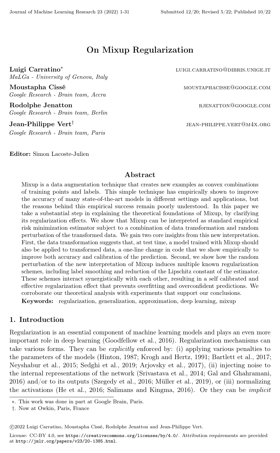
Cover for On Mixup Regularization

Abstract

Mixup is a data augmentation technique that creates new examples as convex combinations of training points and labels. This simple technique has empirically shown to improve the accuracy of many state-of-the-art models in different settings and applications, but the reasons behind this empirical success remain poorly understood. In this paper we take a substantial step in explaining the theoretical foundations of Mixup, by clarifying its regularization effects. We show that Mixup can be interpreted as standard empirical risk minimization estimator subject to a combination of data transformation and random perturbation of the transformed data. We gain two core insights from this new interpretation. First, the data transformation suggests that, at test time, a model trained with Mixup should also be applied to transformed data, a one-line change in code that we show empirically to improve both accuracy and calibration of the prediction. Second, we show how the random perturbation of the new interpretation of Mixup induces multiple known regularization schemes, including label smoothing and reduction of the Lipschitz constant of the estimator. These schemes interact synergistically with each other, resulting in a self calibrated and effective regularization effect that prevents overfitting and overconfident predictions. We corroborate our theoretical analysis with experiments that support our conclusions.

Table of Contents

  • 1. Introduction
  • 2. Notations and setting
  • 3. Mixup as a perturbed ERM
  • 4. The regularization effects of Mixup
  • 5. Discussion and experiments
  • 6. Conclusions
  • Acknowledgments
  • Appendix
  • Appendix A. Proofs
  • A.1 Proof of Theorem 1
  • A.2 Proof of Lemma 2
  • A.3 Proof of Theorem 3
  • A.4 Proof of Corollary 4
  • A.5 Proof of Corollary 5
  • A.6 Proof of Corollary 6
  • A.7 Proof of Proposition 7
  • Appendix B. Experiments
  • B.1 CIFAR-10 and CIFAR-100
  • B.2 ImageNet
  • B.3 Two Moons with Random Features
  • References

Knowls

  1. Knowl 1 — Mixup is ERM on contracted data with structured zero-mean noise

    theoretical result

    Let the training data be (xi,yi)i=1n(x_i,y_i)_{i=1}^n, with means xˉ=n−1∑ixi\bar{x}=n^{-1}\sum_i x_i and yˉ=n−1∑iyi\bar{y}=n^{-1}\sum_i y_i. Standard Mixup uses a mixing weight λ∼Beta(α,α)\lambda\sim\mathrm{Beta}(\alpha,\alpha) and minimizes the average loss on pairwise convex combinations of inputs and labels. Equivalently, draw θ∼Beta[1/2,1](α,α)\theta\sim\mathrm{Beta}_{[1/2,1]}(\alpha,\alpha), independently draw jj uniformly from {1,…,n}\{1,\ldots,n\}, and write m=E[θ]m=\mathbb{E}[\theta]. For each fixed training index ii, define contracted data and random perturbations by

    x~i=xˉ+m(xi−xˉ),y~i=yˉ+m(yi−yˉ),\tilde{x}_i=\bar{x}+m(x_i-\bar{x}),\qquad \tilde{y}_i=\bar{y}+m(y_i-\bar{y}), δi=(θ−m)xi+(1−θ)xj−(1−m)xˉ,εi=(θ−m)yi+(1−θ)yj−(1−m)yˉ.\delta_i=(\theta-m)x_i+(1-\theta)x_j-(1-m)\bar{x},\qquad \varepsilon_i=(\theta-m)y_i+(1-\theta)y_j-(1-m)\bar{y}.

    Both perturbations have mean zero over (θ,j)(\theta,j). For any predictor ff and loss ℓ\ell, the exact Mixup risk is

    EMixup(f)=1n∑i=1nEθ,j[ℓ ⁣(y~i+εi,f(x~i+δi))].\mathcal{E}_{\mathrm{Mixup}}(f)=\frac{1}{n}\sum_{i=1}^n\mathbb{E}_{\theta,j}\left[\ell\!\left(\tilde{y}_i+\varepsilon_i, f(\tilde{x}_i+\delta_i)\right)\right].

    Thus Mixup exactly trains on inputs and labels contracted toward their training means, with jointly generated noise added to both.

  2. Knowl 2 — Mixup noise has explicit, correlated input and output covariances

    equation

    For the contracted training pair (x~i,y~i)(\tilde{x}_i,\tilde{y}_i) and the zero-mean Mixup perturbations (δi,εi)(\delta_i,\varepsilon_i), let σ2=Var⁡(θ)\sigma^2=\operatorname{Var}(\theta), where θ∼Beta[1/2,1](α,α)\theta\sim\mathrm{Beta}_{[1/2,1]}(\alpha,\alpha), and set γ2=σ2+(1−m)2\gamma^2=\sigma^2+(1-m)^2, with m=E[θ]m=\mathbb{E}[\theta]. Define empirical covariances Σxx=n−1∑k(xk−xˉ)(xk−xˉ)⊤\Sigma_{xx}=n^{-1}\sum_k(x_k-\bar{x})(x_k-\bar{x})^\top, Σyy=n−1∑k(yk−yˉ)(yk−yˉ)⊤\Sigma_{yy}=n^{-1}\sum_k(y_k-\bar{y})(y_k-\bar{y})^\top, and Σxy=n−1∑k(xk−xˉ)(yk−yˉ)⊤\Sigma_{xy}=n^{-1}\sum_k(x_k-\bar{x})(y_k-\bar{y})^\top. The perturbation covariance matrices are

    Ai=E[δiδi⊤]=σ2(x~i−xˉ)(x~i−xˉ)⊤+γ2Σx~x~m2,A_i=\mathbb{E}[\delta_i\delta_i^\top]=\frac{\sigma^2(\tilde{x}_i-\bar{x})(\tilde{x}_i-\bar{x})^\top+\gamma^2\Sigma_{\tilde{x}\tilde{x}}}{m^2}, Bi=E[εiεi⊤]=σ2(y~i−yˉ)(y~i−yˉ)⊤+γ2Σy~y~m2,Ci=E[δiεi⊤]=σ2(x~i−xˉ)(y~i−yˉ)⊤+γ2Σx~y~m2.B_i=\mathbb{E}[\varepsilon_i\varepsilon_i^\top]=\frac{\sigma^2(\tilde{y}_i-\bar{y})(\tilde{y}_i-\bar{y})^\top+\gamma^2\Sigma_{\tilde{y}\tilde{y}}}{m^2}, \qquad C_i=\mathbb{E}[\delta_i\varepsilon_i^\top]=\frac{\sigma^2(\tilde{x}_i-\bar{x})(\tilde{y}_i-\bar{y})^\top+\gamma^2\Sigma_{\tilde{x}\tilde{y}}}{m^2}.

    Here Σx~x~=m2Σxx\Sigma_{\tilde{x}\tilde{x}}=m^2\Sigma_{xx}, Σy~y~=m2Σyy\Sigma_{\tilde{y}\tilde{y}}=m^2\Sigma_{yy}, and Σx~y~=m2Σxy\Sigma_{\tilde{x}\tilde{y}}=m^2\Sigma_{xy}. In particular, Mixup does not perturb inputs and outputs independently: CiC_i captures their shared, data-dependent correlation.

  3. Knowl 3 — A quadratic approximation expresses Mixup as modified-data ERM plus four corrections

    theoretical result

    Let f:Rd→Rcf:\mathbb{R}^d\to\mathbb{R}^c and let ℓ(y,u)\ell(y,u) be a twice continuously differentiable loss, where y,u∈Rcy,u\in\mathbb{R}^c. At each contracted pair (x~i,y~i)(\tilde{x}_i,\tilde{y}_i), define Ai=E[δiδi⊤]A_i=\mathbb{E}[\delta_i\delta_i^\top], Bi=E[εiεi⊤]B_i=\mathbb{E}[\varepsilon_i\varepsilon_i^\top], and Ci=E[δiεi⊤]C_i=\mathbb{E}[\delta_i\varepsilon_i^\top] for the Mixup perturbations. Replacing the loss on each perturbed pair by its second-order Taylor approximation around (x~i,y~i)(\tilde{x}_i,\tilde{y}_i) gives

    EMixupQ(f)=1n∑i=1nℓ(y~i,f(x~i))+R1(f)+R2(f)+R3(f)+R4(f).\mathcal{E}_{\mathrm{Mixup}}^{Q}(f)=\frac{1}{n}\sum_{i=1}^n\ell(\tilde{y}_i,f(\tilde{x}_i))+R_1(f)+R_2(f)+R_3(f)+R_4(f).

    Write Di=∇f(x~i)∈Rc×dD_i=\nabla f(\tilde{x}_i)\in\mathbb{R}^{c\times d}, Hi=∇uu2ℓ(y~i,f(x~i))H_i=\nabla^2_{uu}\ell(\tilde{y}_i,f(\tilde{x}_i)), and Ki=∇uy2ℓ(y~i,f(x~i))K_i=\nabla^2_{uy}\ell(\tilde{y}_i,f(\tilde{x}_i)). Where the required inverses exist, set Ji=−Hi−1KiCi⊤Ai−1J_i=-H_i^{-1}K_iC_i^\top A_i^{-1}. The four terms are

    R1=12n∑itr⁡ ⁣[Hi(Di−Ji)Ai(Di−Ji)⊤],R2=12n∑i⟨Ai,∑k=1c∂ℓ∂uk∇2fk(x~i)⟩,R_1=\frac{1}{2n}\sum_i\operatorname{tr}\!\left[H_i(D_i-J_i)A_i(D_i-J_i)^\top\right],\qquad R_2=\frac{1}{2n}\sum_i\left\langle A_i,\sum_{k=1}^c\frac{\partial\ell}{\partial u_k}\nabla^2 f_k(\tilde{x}_i)\right\rangle, R3=−12n∑itr⁡(Ai−1CiHi−1Ci⊤),R4=12n∑i⟨Bi,∇yy2ℓ(y~i,f(x~i))⟩.R_3=-\frac{1}{2n}\sum_i\operatorname{tr}(A_i^{-1}C_iH_i^{-1}C_i^\top),\qquad R_4=\frac{1}{2n}\sum_i\left\langle B_i,\nabla^2_{yy}\ell(\tilde{y}_i,f(\tilde{x}_i))\right\rangle.

    The derivatives in R2R_2 are evaluated at (y~i,f(x~i))(\tilde{y}_i,f(\tilde{x}_i)); fkf_k is the kkth output component, and ⟨⋅,⋅⟩\langle\cdot,\cdot\rangle is the Frobenius inner product. The approximation therefore separates ERM on contracted data from corrections due to input curvature, output curvature, input-output noise correlation, and the discrepancy between the model Jacobian and the covariance-dependent target JiJ_i.

  4. Knowl 4 — Cross-entropy Mixup couples label smoothing to Jacobian regularization

    model/method

    For multiclass cross-entropy with softmax probabilities pi=softmax⁡(f(x~i))p_i=\operatorname{softmax}(f(\tilde{x}_i)), the output Hessian is Hi=diag⁡(pi)−pipi⊤H_i=\operatorname{diag}(p_i)-p_ip_i^\top, and the contracted target is y~i=yˉ+m(yi−yˉ)\tilde{y}_i=\bar{y}+m(y_i-\bar{y}). In the quadratic Mixup approximation, the nonzero corrections have the form

    R1=12n∑itr⁡ ⁣[Hi(Di−Ji)Ai(Di−Ji)⊤],Ji=Hi−1Ci⊤Ai−1,R_1=\frac{1}{2n}\sum_i\operatorname{tr}\!\left[H_i(D_i-J_i)A_i(D_i-J_i)^\top\right],\qquad J_i=H_i^{-1}C_i^\top A_i^{-1}, R2=12n∑i⟨Ai,∑k=1c(pik−y~ik)∇2fk(x~i)⟩,R3=−12n∑itr⁡(Ai−1CiHi−1Ci⊤).R_2=\frac{1}{2n}\sum_i\left\langle A_i,\sum_{k=1}^c(p_{ik}-\tilde{y}_{ik})\nabla^2 f_k(\tilde{x}_i)\right\rangle, \qquad R_3=-\frac{1}{2n}\sum_i\operatorname{tr}(A_i^{-1}C_iH_i^{-1}C_i^\top).

    Here AiA_i is the input-noise covariance, CiC_i is the input-output noise cross-covariance, and Di=∇f(x~i)D_i=\nabla f(\tilde{x}_i). Cross-entropy is linear in its target, so its output-only curvature term is zero. The first correction penalizes deviation of the model Jacobian from a linear-regression-like target JiJ_i, rather than simply penalizing the Jacobian norm. This penalty is weighted by the softmax Hessian and can weaken for highly confident predictions. Mixup also smooths targets toward the mean label, which tends to discourage such confidence and can keep the Jacobian penalty active. The two effects arise together from Mixup's correlated input and output perturbations.

  5. Knowl 5 — Label smoothing gives an entropy bound for linear cross-entropy classifiers

    theoretical result

    Consider a multiclass dataset with one-hot targets yi∈Rcy_i\in\mathbb{R}^c, mean target yˉ=n−1∑iyi\bar{y}=n^{-1}\sum_i y_i, and linear logits f(x)=Wxf(x)=Wx. Let W∗W^* minimize average cross-entropy on the original targets and let Wsm∗W^*_{\mathrm{sm}} minimize it on the smoothed targets y~i=yˉ+m(yi−yˉ)\tilde{y}_i=\bar{y}+m(y_i-\bar{y}), where m∈[0,1]m\in[0,1]. Define pi=softmax⁡(W∗xi)p_i=\operatorname{softmax}(W^*x_i) and p~i=softmax⁡(Wsm∗xi)\tilde{p}_i=\operatorname{softmax}(W^*_{\mathrm{sm}}x_i), and let Z(p)=−∑k=1cpklog⁡pkZ(p)=-\sum_{k=1}^c p_k\log p_k be categorical entropy. The paper establishes

    m1n∑i=1nZ(pi)+(1−m)Z(yˉ)≤1n∑i=1nZ(p~i).m\frac{1}{n}\sum_{i=1}^n Z(p_i)+(1-m)Z(\bar{y})\leq\frac{1}{n}\sum_{i=1}^n Z(\tilde{p}_i).

    Consequently, if the original classifier's average prediction entropy is at most Z(yˉ)Z(\bar{y}), label smoothing increases or preserves the average prediction entropy. This result applies to the stated linear-model, cross-entropy optimization setting; it is not an unconditional entropy comparison for arbitrary predictors.

  6. Knowl 6 — Test-time evaluation should undo Mixup's input and output contraction

    model/method

    A predictor ff trained with Mixup is fit to inputs and targets contracted toward the training means, rather than directly to the original input and output coordinates. Let xˉ\bar{x} and yˉ\bar{y} be those training means and let m=E[θ]m=\mathbb{E}[\theta] for θ∼Beta[1/2,1](α,α)\theta\sim\mathrm{Beta}_{[1/2,1]}(\alpha,\alpha), using the training Mixup parameter α\alpha. For a test input xx, the corresponding prediction in the original output coordinates is

    pred⁡f(x)=yˉ(1−1m)+1mf(mx+(1−m)xˉ).\operatorname{pred}_f(x)=\bar{y}\left(1-\frac{1}{m}\right)+\frac{1}{m}f\bigl(mx+(1-m)\bar{x}\bigr).

    Thus evaluation first contracts the test input toward the training input mean, applies the trained predictor, and then maps its output back from the contracted output coordinates. If the training data are centered and ff is positively homogeneous, this correction leaves predictions unchanged. With balanced classes, the output correction adds a common offset to all logits; because softmax ignores a common offset, the procedure is equivalent to scaling logits by 1/m1/m.

  7. Knowl 7 — Mixup does not change the ordinary least-squares solution for linear regression

    theoretical result

    For squared-error regression with a linear predictor and intercept, fW,b(x)=Wx+bf_{W,b}(x)=Wx+b, the loss is quadratic in the input and target, so the second-order perturbation approximation is exact. The exact Mixup risk has the same minimizing linear predictor as ordinary empirical risk minimization on the original data: its slope and intercept are the standard multivariate ordinary least-squares solution. Therefore, in this setting Mixup does not alter the fitted predictor, even though it changes the risk's scaling and adds terms that do not change the minimizer.

  8. Knowl 8 — The proposed test-time correction improves in-distribution evaluation in most tested settings

    empirical result

    The authors compared standard Mixup with Mixup followed by the test-time contraction-and-expansion correction on CIFAR-10 and CIFAR-100 using ResNet-34, and on ImageNet using ResNet-50. They evaluated test accuracy, cross-entropy loss, and expected calibration error (ECE); results were averaged over 10 repetitions for CIFAR and 5 for ImageNet. On CIFAR-10 and CIFAR-100, corrected Mixup generally gave higher accuracy and lower loss and ECE than uncorrected Mixup across the tested mixing strengths. On ImageNet, the overall pattern was also favorable, with the reported exception that loss and ECE did not improve for very small α\alpha. Applying the same correction to ERM-trained models instead deteriorated performance, supporting the authors' claim that the correction is specific to the contracted coordinates induced by Mixup.

  9. Knowl 9 — The quadratic approximation tracks Mixup behavior but omits an unstable curvature term

    empirical result

    On CIFAR-10 with LeNet, the authors compared training with the exact Mixup risk against training with its quadratic regularized-ERM approximation. In the approximation experiment they omitted the Hessian-related term R2R_2, reporting that it caused numerical instability because of its non-convexity. The approximate objective nevertheless produced training and test loss and accuracy trajectories that closely followed those of standard Mixup. A further comparison among Mixup, ERM, and ERM on contracted data found that Mixup-trained functions had the smallest values of the approximation's regularization terms, but not the smallest loss on contracted data. The result supports the approximation as a qualitative account of Mixup's regularization trade-off, not as an exact replacement for Mixup in all settings.

  10. Knowl 10 — Test-time correction has mixed results on out-of-distribution data

    limitation

    The theoretical test-time correction is derived for the in-distribution training-and-test setting, and its out-of-distribution (OOD) behavior was assessed empirically. The experiments used CIFAR-10-C and CIFAR-100-C corruption benchmarks, as well as ImageNet-derived OOD benchmarks, with models trained on the corresponding uncorrupted dataset. Rescaling improved some metrics on several ImageNet-derived sets, but on CIFAR-10-C, CIFAR-100-C, and ImageNet-C it worsened almost all reported metrics relative to standard Mixup. On CIFAR-C, the performance gap increasingly favored uncorrected Mixup as corruption intensity increased; the corruption analysis averaged over 19 corruption types at each of five severity levels. Thus the correction's in-distribution benefits do not establish an OOD benefit, and severe input corruption can reverse its effect.

Coverage note — Supplementary training schedules and the synthetic two-moons random-feature experiment are omitted because they repeat the paper's main empirical patterns rather than adding a distinct central result.

References

  1. 1.Martin Arjovsky, Soumith Chintala, and Léon Bottou. Wasserstein GAN. arXiv preprint arXiv:1701.07875, 2017.
  2. 2.Sanjeev Arora, Nadav Cohen, Wei Hu, and Yuping Luo. Implicit regularization in deep matrix factorization. In H. Wallach, H. Larochelle, A. Beygelzimer, F. d’Alché Buc, E. Fox, and R. Garnett, editors, Advances in Neural Information Processing Systems, volume 32, pages 7411–7422. Curran Associates, Inc., 2019.
  3. 3.Devansh Arpit, Stanisław Jastrzębski, Nicolas Ballas, David Krueger, Emmanuel Bengio, Maxinder S Kanwal, Tegan Maharaj, Asja Fischer, Aaron Courville, Yoshua Bengio, and Simon Lacoste-Julien. A closer look at memorization in deep networks. In Proceedings of the 34th International Conference on Machine Learning-Volume 70, pages 233–242. JMLR.org, 2017.
  4. 4.Andrei Barbu, David Mayo, Julian Alverio, William Luo, Christopher Wang, Dan Gutfreund, Josh Tenenbaum, and Boris Katz. ObjectNet: A large-scale bias-controlled dataset for pushing the limits of object recognition models. In H. Wallach, H. Larochelle, A. Beygelzimer, F. d’Alché Buc, E. Fox, and R. Garnett, editors, Advances in Neural Information Processing Systems, volume 32, pages 9453–9463. Curran Associates, Inc., 2019.
  5. 5.Peter L Bartlett, Dylan J Foster, and Matus J Telgarsky. Spectrally-normalized margin bounds for neural networks. In Proceedings of the 31st International Conference on Neural Information Processing Systems, page 6241–6250. Curran Associates Inc., 2017.
  6. 6.David Berthelot, Nicholas Carlini, Ian Goodfellow, Nicolas Papernot, Avital Oliver, and Colin Raffel. MixMatch: A holistic approach to semi-supervised learning. In Proceedings of the 33rd International Conference on Neural Information Processing Systems. Curran Associates Inc., 2019.
  7. 7.Chris M Bishop. Training with noise is equivalent to Tikhonov regularization. Neural computation, 7(1):108–116, 1995.
  8. 8.Léon Bottou and Olivier Bousquet. The tradeoffs of large scale learning. In J. C. Platt, D. Koller, Y. Singer, and S. T. Roweis, editors, Advances in Neural Information Processing Systems, volume 20, pages 161–168. Curran Associates, Inc., 2008.
  9. 9.Stephen P Boyd and Lieven Vandenberghe. Convex optimization. Cambridge University Press, 2004.
  10. 10.Luigi Carratino, Moustapha Cissé, Rodolphe Jenatton, and Jean-Philippe Vert. On mixup regularization. Technical Report 2006.06049, arXiv, 2020.
  11. 11.Moustapha Cissé, Piotr Bojanowski, Edouard Grave, Yann Dauphin, and Nicolas Usunier. Parseval networks: Improving robustness to adversarial examples. In Proceedings of the 34th International Conference on Machine Learning-Volume 70, pages 854–863. JMLR.org, 2017.
  12. 12.Yarin Gal and Zoubin Ghahramani. Dropout as a Bayesian approximation: Representing model uncertainty in deep learning. In Maria Florina Balcan and Kilian Q. Weinberger, editors, Proceedings of The 33rd International Conference on Machine Learning, volume 48 of Proceedings of Machine Learning Research, pages 1050–1059. PMLR, 2016.
  13. 13.Ian Goodfellow, Yoshua Bengio, and Aaron Courville. Deep learning. MIT press, 2016.
  14. 14.Ishaan Gulrajani, Faruk Ahmed, Martin Arjovsky, Vincent Dumoulin, and Aaron C Courville. Improved training of Wasserstein GANs. In I. Guyon, U. Von Luxburg, S. Bengio, H. Wallach, R. Fergus, S. Vishwanathan, and R. Garnett, editors, Advances in Neural Information Processing Systems, volume 30, pages 5767–5777. Curran Associates, Inc., 2017.
  15. 15.Chuan Guo, Geoff Pleiss, Yu Sun, and Kilian Q Weinberger. On calibration of modern neural networks. In Proceedings of the 34th International Conference on Machine Learning-Volume 70, pages 1321–1330. JMLR.org, 2017.
  16. 16.Hongyu Guo. Nonlinear Mixup: Out-of-manifold data augmentation for text classification. In Proceedings of the AAAI Conference on Artificial Intelligence, volume 34, pages 4044–4051, 2020.
  17. 17.Hongyu Guo, Yongyi Mao, and Richong Zhang. Mixup as locally linear out-of-manifold regularization. In Proceedings of the AAAI Conference on Artificial Intelligence, volume 33, pages 3714–3722, 2019.
  18. 18.Kaiming He, Xiangyu Zhang, Shaoqing Ren, and Jian Sun. Deep residual learning for image recognition. In Proceedings of the IEEE conference on computer vision and pattern recognition, pages 770–778, 2016.
  19. 19.Matthias Hein and Maksym Andriushchenko. Formal guarantees on the robustness of a classifier against adversarial manipulation. In Proceedings of the 31st International Conference on Neural Information Processing Systems, page 2263–2273. Curran Associates Inc., 2017.
  20. 20.Dan Hendrycks and Thomas G. Dietterich. Benchmarking neural network robustness to common corruptions and perturbations. In 7th International Conference on Learning Representations, ICLR 2019, New Orleans, LA, USA, May 6-9, 2019. OpenReview.net, 2019.
  21. 21.Dan Hendrycks and Kevin Gimpel. A baseline for detecting misclassified and out-of-distribution examples in neural networks. In 5th International Conference on Learning Representations, ICLR 2017, Toulon, France, April 24-26, 2017, Conference Track Proceedings. OpenReview.net, 2017.
  22. 22.Dan Hendrycks, Kevin Zhao, Steven Basart, Jacob Steinhardt, and Dawn Song. Natural adversarial examples. In IEEE Conference on Computer Vision and Pattern Recognition, CVPR 2021, virtual, June 19-25, 2021, pages 15262–15271. Computer Vision Foundation / IEEE, 2021.
  23. 23.Geoffrey E Hinton. Learning translation invariant recognition in a massively parallel networks. In International Conference on Parallel Architectures and Languages Europe, pages 1–13. Springer, 1987.
  24. 24.Beyrem Khalfaoui, Joseph Boyd, and Jean-Philippe Vert. Asni: Adaptive structured noise injection for shallow and deep neural networks. arXiv preprint arXiv:1909.09819, 2019.
  25. 25.Anders Krogh and John A Hertz. A simple weight decay can improve generalization. In J. Moody, S. Hanson, and R.P. Lippmann, editors, Advances in neural information processing systems, volume 4, pages 950–957. Morgan-Kaufmann, 1991.
  26. 26.Yann LeCun, Léon Bottou, Yoshua Bengio, and Patrick Haffner. Gradient-based learning applied to document recognition. Proceedings of the IEEE, 86(11):2278–2324, 1998.
  27. 27.Rafael Müller, Simon Kornblith, and Geoffrey E Hinton. When does label smoothing help? In H. Wallach, H. Larochelle, A. Beygelzimer, F. d’Alché Buc, E. Fox, and R. Garnett, editors, Advances in Neural Information Processing Systems 32, pages 4694–4703. Curran Associates, Inc., 2019.
  28. 28.Behnam Neyshabur. Implicit regularization in deep learning. arXiv preprint arXiv:1709.01953, 2017.
  29. 29.Behnam Neyshabur, Russ R Salakhutdinov, and Nati Srebro. Path-SGD: Path-normalized optimization in deep neural networks. In Proceedings of the 28th International Conference on Neural Information Processing Systems - Volume 2, pages 2422–2430, 2015.
  30. 30.Gabriel Pereyra, George Tucker, Jan Chorowski, Łukasz Kaiser, and Geoffrey Hinton. Regularizing neural networks by penalizing confident output distributions. In 5th International Conference on Learning Representations, ICLR 2017, Toulon, France, April 24-26, 2017, Workshop Track Proceedings. OpenReview.net, 2017.
  31. 31.Ali Rahimi and Benjamin Recht. Random features for large-scale kernel machines. In J. Platt, D. Koller, Y. Singer, and S. Roweis, editors, Advances in neural information processing systems, volume 20, pages 1177–1184. Curran Associates, Inc., 2008.
  32. 32.Benjamin Recht, Rebecca Roelofs, Ludwig Schmidt, and Vaishaal Shankar. Do ImageNet classifiers generalize to ImageNet? In Kamalika Chaudhuri and Ruslan Salakhutdinov, editors, Proceedings of the 36th International Conference on Machine Learning, volume 97, pages 5389–5400. PMLR, 2019.
  33. 33.Tim Salimans and Durk P Kingma. Weight normalization: A simple reparameterization to accelerate training of deep neural networks. In D. Lee, M. Sugiyama, U. Luxburg, I. Guyon, and R. Garnett, editors, Advances in neural information processing systems, volume 29, pages 901–909. Curran Associates, Inc., 2016.
  34. 34.Hanie Sedghi, Vineet Gupta, and Philip M Long. The singular values of convolutional layers. In 7th International Conference on Learning Representations, ICLR 2019, New Orleans, LA, USA, May 6-9, 2019. OpenReview.net, 2019.
  35. 35.Vaishaal Shankar, Achal Dave, Rebecca Roelofs, Deva Ramanan, Benjamin Recht, and Ludwig Schmidt. Do image classifiers generalize across time? In ICCV, pages 9641–9649. IEEE, 2021.
  36. 36.Nitish Srivastava, Geoffrey Hinton, Alex Krizhevsky, Ilya Sutskever, and Ruslan Salakhutdinov. Dropout: a simple way to prevent neural networks from overfitting. The Journal of Machine Learning Research, 15(1):1929–1958, 2014.
  37. 37.Christian Szegedy, Vincent Vanhoucke, Sergey Ioffe, Jon Shlens, and Zbigniew Wojna. Rethinking the inception architecture for computer vision. In Proceedings of the IEEE conference on computer vision and pattern recognition, pages 2818–2826, 2016.
  38. 38.Sunil Thulasidasan, Gopinath Chennupati, Jeff A Bilmes, Tanmoy Bhattacharya, and Sarah Michalak. On mixup training: Improved calibration and predictive uncertainty for deep neural networks. In H. Wallach, H. Larochelle, A. Beygelzimer, F. d’Alché Buc, E. Fox, and R. Garnett, editors, Advances in Neural Information Processing Systems, volume 32. Curran Associates, Inc., 2019.
  39. 39.Yuji Tokozume, Yoshitaka Ushiku, and Tatsuya Harada. Between-class learning for image classification. In Proceedings of the IEEE Conference on Computer Vision and Pattern Recognition, pages 5486–5494, 2018.
  40. 40.Vikas Verma, Alex Lamb, Christopher Beckham, Amir Najafi, Ioannis Mitliagkas, David Lopez-Paz, and Yoshua Bengio. Manifold mixup: Better representations by interpolating hidden states. In Kamalika Chaudhuri and Ruslan Salakhutdinov, editors, Proceedings of the 36th International Conference on Machine Learning, volume 97 of Proceedings of Machine Learning Research, pages 6438–6447, Long Beach, California, USA, 09–15 Jun 2019. PMLR. URL http://proceedings.mlr.press/v97/verma19a.html.
  41. 41.Stefan Wager, Sida Wang, and Percy S Liang. Dropout training as adaptive regularization. In C.J. Burges, L. Bottou, M. Welling, Z. Ghahramani, and K.Q. Weinberger, editors, Advances in neural information processing systems, volume 26, pages 351–359. Curran Associates, Inc., 2013.
  42. 42.Colin Wei, Sham Kakade, and Tengyu Ma. The implicit and explicit regularization effects of dropout. In Hal Daumé III and Aarti Singh, editors, Proceedings of the 37th International Conference on Machine Learning, volume 119 of Proceedings of Machine Learning Research, pages 10181–10192. PMLR, 13–18 Jul 2020.
  43. 43.Sangdoo Yun, Dongyoon Han, Seong Joon Oh, Sanghyuk Chun, Junsuk Choe, and Youngjoon Yoo. Cutmix: Regularization strategy to train strong classifiers with localizable features. In Proceedings of the IEEE International Conference on Computer Vision, pages 6023–6032, 2019.
  44. 44.Hongyi Zhang, Moustapha Cissé, Yann N. Dauphin, and David Lopez-Paz. mixup: Beyond empirical risk minimization. In 6th International Conference on Learning Representations, ICLR 2018, Vancouver, BC, Canada, April 30 - May 3, 2018, Conference Track Proceedings, 2018.
  45. 45.Linjun Zhang, Zhun Deng, Kenji Kawaguchi, Amirata Ghorbani, and James Zou. How does mixup help with robustness and generalization? In International Conference on Learning Representations. OpenReview.net, 2021.

Citation

MLA
Carratino, L., et al. “On Mixup Regularization”. Journal of Machine Learning Research, vol. 23, no. 325, 2022, pp. 1–1, https://www.jmlr.org/papers/v23/20-1385.html.
APA
Carratino, L., Cissé, M., Jenatton, R., & Vert, J.-P. (2022). On Mixup Regularization. Journal of Machine Learning Research, 23(325), 1–31. https://www.jmlr.org/papers/v23/20-1385.html
Chicago
Carratino, L., M. Cissé, R. Jenatton, and J.-P. Vert. 2022. “On Mixup Regularization”. Journal of Machine Learning Research 23 (325): 1–31. https://www.jmlr.org/papers/v23/20-1385.html.
Harvard
Carratino, L. et al. (2022) “On Mixup Regularization”, Journal of Machine Learning Research, 23(325), pp. 1–31. Available at: https://www.jmlr.org/papers/v23/20-1385.html.
Vancouver
1. Carratino L, Cissé M, Jenatton R, Vert J-P (2022) On Mixup Regularization. Journal of Machine Learning Research 23:1–31

BibTeX

@article{JMLR:v23:20-1385,
  author  = {Luigi Carratino and Moustapha Cissé and Rodolphe Jenatton and Jean-Philippe Vert},
  title   = {On Mixup Regularization},
  journal = {Journal of Machine Learning Research},
  year    = {2022},
  volume  = {23},
  number  = {325},
  pages   = {1--31},
  url     = {http://jmlr.org/papers/v23/20-1385.html}
}
Metadata:DOI registry

Access the Paper

This paper is available from its original source. Click below to access the PDF.

Open PDF
License: https://creativecommons.org/licenses/by/4.0/