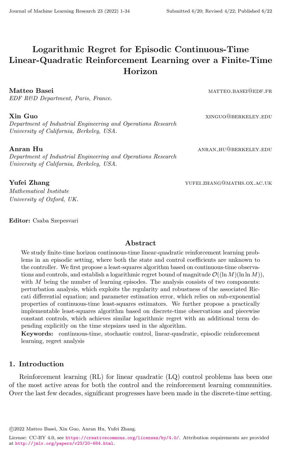
Logarithmic Regret for Episodic Continuous-Time Linear-Quadratic Reinforcement Learning over a Finite-Time Horizon

Matteo BaseiXin GuoAnran HuYufei Zhang

article2022JMLR53 citations

Establishes the first near-logarithmic regret bounds for episodic continuous-time linear-quadratic reinforcement learning with unknown dynamics, providing both theoretical guarantees via Riccati differential equation analysis and a practical discrete-time implementation that quantifies the impact of discretization stepsizes.

Listen

Many critical real-world control systems, such as those in robotics, aerospace, autonomous vehicles, and algorithmic trading, operate naturally in continuous time. While reinforcement learning for discrete-time linear-quadratic control has seen significant progress, practical deployments in continuous environments often suffer from performance degradation and lack non-asymptotic performance guarantees when discrete-time algorithms are applied.

The article aims to design and theoretically validate reinforcement learning algorithms for continuous-time linear-quadratic control over a finite-time horizon when both state and control system parameters are unknown. It evaluates whether greedy, least-squares-based methods can achieve non-asymptotic logarithmic regret in both continuous-time and practical discrete-time settings.

The authors analyze two least-squares-based learning algorithms operating in episodic cycles where the number of episodes doubles each cycle. The first algorithm assumes continuous-time observations and controls, while the second uses discrete-time observations and piecewise-constant controls. The methodological framework combines perturbation analysis of continuous-time and discrete-time Riccati equations, concentration inequalities exploiting the sub-exponential tail behavior of least-squares estimators, and self-exploration properties inherent to finite-horizon continuous-time linear-quadratic systems.

The article establishes several key findings. First, the continuous-time least-squares algorithm achieves a logarithmic regret bound of magnitude O((ln M)(ln ln M)), where M is the number of learning episodes, representing the first non-asymptotic logarithmic regret bound for continuous-time linear-quadratic reinforcement learning with unknown state and control parameters. Second, finite-horizon continuous-time systems exhibit an intrinsic self-exploration property driven by time-dependent feedback matrices and continuous Brownian noise, eliminating the need for artificial exploratory noise. Third, the practical discrete-time algorithm achieves a similar logarithmic regret bound with an added discretization penalty; if the time grid stepsize is held fixed, the regret degrades to linear O(M), but if the number of time intervals grows appropriately across cycles, logarithmic regret is fully preserved. Fourth, scaling the regularization hyperparameter linearly with the time stepsize is essential to prevent estimator degeneration as the sampling stepsize approaches zero.

These findings provide rigorous guidance for engineering cyber-physical and automated control systems. Implementing reinforcement learning in continuous environments without adjusting the observation frequency or hyperparameter scaling across timescales risks severe performance loss. By demonstrating that greedy certainty-equivalent control is sufficient without added exploration, the results simplify controller implementation and reduce tracking costs and operational risks.

Decision-makers and engineering teams should adopt timescale-scaled regularization parameters when deploying discrete-time learning controllers into continuous-time physical systems. Furthermore, control architectures should employ time discretization schedules that refine the observation frequency across learning cycles to maintain optimal logarithmic regret scaling.

The theoretical guarantees assume that the system satisfies an identifiability condition ensuring the optimal policy excites all parameter directions, and the regret bounds depend exponentially on the total time horizon T. While confidence in the mathematical derivations is high for finite-horizon settings, practitioners should exercise caution when extrapolating these bounds to very long time horizons without further stabilizability analysis.

Department of Industrial Engineering and Operations Research Électricité de France Mathematical Institute University of California Berkeley University of Oxford continuous time control parameters discrete-time continuous-time linear-quadratic reinforcement learning logarithmic regret finite-time horizon

arXiv: 2006.15316

No sufficiently relevant recommendations were found.

Cover for Logarithmic Regret for Episodic Continuous-Time Linear-Quadratic Reinforcement Learning over a Finite-Time Horizon

Abstract

We study finite-time horizon continuous-time linear-quadratic reinforcement learning problems in an episodic setting, where both the state and control coefficients are unknown to the controller. We first propose a least-squares algorithm based on continuous-time observations and controls, and establish a logarithmic regret bound of magnitude O((ln M)(ln ln M)), with M being the number of learning episodes. The analysis consists of two components: perturbation analysis, which exploits the regularity and robustness of the associated Riccati differential equation; and parameter estimation error, which relies on sub-exponential properties of continuous-time least-squares estimators. We further propose a practically implementable least-squares algorithm based on discrete-time observations and piecewise constant controls, which achieves similar logarithmic regret with an additional term depending explicitly on the time stepsizes used in the algorithm.

Topics

continuous time control parameters discrete-time equivalent control finite time optimal policies performance guarantees perturbation analysis regularization parameters self-driving auto

Keywords

continuous-time linear-quadratic reinforcement learning logarithmic regret finite-time horizon certainty equivalent control continuous-time least-squares algorithm continuous-time Riccati equation stochastic control Thompson sampling

1. Introduction
1.1 Discrete-Time RL
1.2 Continuous-Time RL
2. Problem Formulation and Main Results
2.1 Linear-Quadratic Reinforcement Learning problem
2.2 Continuous-Time Least-Squares Algorithm and Its Regret Bound
2.3 Discrete-Time Least-Squares Algorithm and Its Regret Bound
3. Proofs of Theorems 2.2 and 2.3
3.1 Convergence and Stability of Riccati Equations and Feedback Controls
3.2 Concentration Inequalities for Least-Squares Estimators
3.3 Regret Analysis of Continuous-Time Least-Squares Algorithm
3.4 Regret Analysis of Discrete-Time Least-Squares Algorithm
References

Knowls

Knowl 1 — Finite-horizon continuous-time LQ learning problem and regret
model/method
The paper studies episodic learning for a stochastic linear system whose drift matrices are unknown. On each episode, the state $X_t\in\mathbb{R}^n$ and control $U_t\in\mathbb{R}^d$ satisfy
$dX_t=(A^\star X_t+B^\star U_t)\,dt+dW_t,\qquad X_0=x_0,\quad t\in[0,T],$
where $A^\star\in\mathbb{R}^{n\times n}$ and $B^\star\in\mathbb{R}^{n\times d}$ are unknown, $W$ is an $n$ -dimensional standard Brownian motion, and the initial state $x_0$ and finite horizon $T$ are given. The running cost uses $Q\succeq0$ and $R\succ0$ :
$J^{\theta^\star}(U)=\mathbb{E}\!\left[\int_0^T(X_t^\top QX_t+U_t^\top RU_t)\,dt\right],\qquad \theta^\star=(A^\star,B^\star)^\top.$
If the matrices were known, the optimal feedback is $U_t=K_t^{\theta^\star}X_t$ , where $K_t^{\theta^\star}=-R^{-1}(B^\star)^\top P_t^{\theta^\star}$ and the matrix $P_t^{\theta^\star}$ solves
$\dot P_t+(A^\star)^\top P_t+P_tA^\star-P_tB^\star R^{-1}(B^\star)^\top P_t+Q=0,\qquad P_T=0.$
For $M$ episodes, the expected regret is the cumulative excess cost over using this known-model optimal feedback on every episode:
$R(M)=\sum_{i=1}^M\bigl(J^{\theta^\star}(U^{\psi_i})-J^{\theta^\star}(U^{\theta^\star})\bigr),$
where $\psi_i$ is the feedback policy used in episode $i$ and $U^{\psi_i}$ is its resulting control.
Knowl 2 — Finite-horizon optimal feedback can identify both unknown drift matrices
theoretical result
For a model parameter $\theta=(A,B)$ , let $K_t^\theta=-R^{-1}B^\top P_t^\theta$ be its finite-horizon optimal feedback, with $P^\theta$ solving the Riccati differential equation with terminal condition $P_T^\theta=0$ . The paper's identifiability condition is
$\{v\in\mathbb{R}^d:(K_t^{\theta^\star})^\top v=0\text{ for every }t\in[0,T]\}=\{0\}.$
Under the paper's finite-horizon LQ assumptions, this is equivalent to positive definiteness of the expected feature Gramian $\mathbb{E}[\int_0^T Z_tZ_t^\top dt]$ , where $Z_t=(X_t^\top,U_t^\top)^\top$ is formed from the true-model optimal state and control. Equivalently, no nonzero pair $(u,v)\in\mathbb{R}^n\times\mathbb{R}^d$ can satisfy $u^\top X_t+v^\top U_t=0$ for almost every time and outcome. The paper attributes this self-exploration property to the time-varying optimal feedback and nondegenerate Brownian noise; it permits exploration-free parameter learning when both $A^\star$ and $B^\star$ are unknown.

Sufficient conditions include $(B^\star)^\top Q B^\star\succ0$ , which ensures identifiability for every $T>0$ . A second sufficient condition applies for all sufficiently large horizons: the algebraic Riccati equation must have a maximal solution $P_\infty^\star$ , the finite-horizon solutions must satisfy $P_0^{\star,(T)}\to P_\infty^\star$ as $T\to\infty$ , and $K_\infty^\star(K_\infty^\star)^\top\succ0$ , where $K_\infty^\star=-R^{-1}(B^\star)^\top P_\infty^\star$ .
Knowl 3 — Continuous-observation regularized least-squares learning algorithm
algorithm
The continuous-time algorithm repeatedly applies a certainty-equivalent finite-horizon LQ feedback and estimates the unknown drift from complete state trajectories. Given an estimate $\theta_\ell=(A_\ell,B_\ell)$ , compute $P^{\theta_\ell}$ from the Riccati equation with terminal value zero and use $U_t=K_t^{\theta_\ell}X_t$ , where $K_t^{\theta_\ell}=-R^{-1}B_\ell^\top P_t^{\theta_\ell}$ . Collect $m_\ell$ independent episodes under this policy. For each trajectory $j$ , define $Z_t^{(j)}=((X_t^{(j)})^\top,(U_t^{(j)})^\top)^\top$ and update by
$\theta_{\ell+1}=\left(\frac{1}{m_\ell}\sum_{j=1}^{m_\ell}\int_0^T Z_t^{(j)}(Z_t^{(j)})^\top dt+\frac{1}{m_\ell}I\right)^{-1} \left(\frac{1}{m_\ell}\sum_{j=1}^{m_\ell}\int_0^T Z_t^{(j)}(dX_t^{(j)})^\top\right),$
where $I$ is the $(n+d)\times(n+d)$ identity. The regularizer makes the empirical inverse well-defined and vanishes as the number of episodes grows. The algorithm starts from an initial estimate $\theta_0$ , repeats these cycles, and can be stopped after the desired number of learning episodes; the policy is unchanged within each cycle.
Knowl 4 — Continuous-time greedy policies have a quadratic cost gap
theoretical result
Let $\theta^\star=(A^\star,B^\star)$ be the true drift parameter and let $\theta=(A,B)$ be an estimated parameter in a bounded set. Apply the finite-horizon optimal feedback computed for $\theta$ to the true system, and denote the resulting control by $U^{\psi^\theta}$ . Under the paper's finite-horizon LQ assumptions, there is a constant $C$ —uniform over the bounded set—such that
$0\le J^{\theta^\star}(U^{\psi^\theta})-J^{\theta^\star}(U^{\theta^\star})\le C\lvert\theta-\theta^\star\rvert^2.$
Thus, model-parameter error affects the cost quadratically when the controller uses the Riccati-based greedy feedback. The bound relies on regularity of the Riccati solution and its feedback with respect to the model parameters.
Knowl 5 — Continuous-time least-squares estimation concentrates at the episode-sample rate
theoretical result
For a current feedback parameter $\theta$ in a bounded neighborhood of $\theta^\star$ , suppose the expected continuous-time feature Gramian $G^\theta=\mathbb{E}[\int_0^T Z_tZ_t^\top dt]$ is uniformly positive definite there and the parameters are bounded. Use $m$ independent full-trajectory episodes under the feedback computed from $\theta$ , and let $\widehat\theta$ be the regularized estimator defined by the empirical Gramian and state-increment integrals. There are constants $C_1,C_2$ such that, for $\delta\in(0,1/2)$ and $m\ge C_1(-\ln\delta)$ ,
$\mathbb{P}\!\left(\lvert\widehat\theta-\theta^\star\rvert\le C_2\left[\sqrt{\frac{-\ln\delta}{m}}+\frac{-\ln\delta}{m}+\frac{(-\ln\delta)^2}{m^2}\right]\right)\ge 1-2\delta.$
The bound follows from concentration of the trajectory-based least-squares statistics; in particular, the stochastic integrals involved have sub-exponential tails. Its uniform Gramian condition is ensured locally when the feedback is identifiable.
Knowl 6 — Continuous-observation algorithm achieves logarithmic regret
empirical result
Assume the true optimal feedback is identifiable and the initial model estimate also has an identifiable feedback. Choose $m_0=C(-\ln\delta)$ episodes in the first cycle and $m_\ell=2^\ell m_0$ episodes in cycle $\ell$ , with $C$ sufficiently large. Then, for $\delta\in(0,3/\pi^2)$ , the continuous-observation least-squares algorithm has, with probability at least $1-\pi^2\delta/3$ , the uniform regret bound
$R(M)\le C'\left[(\ln M)(\ln\ln M)+(-\ln\delta)(\ln M)\right],\qquad M\in\mathbb{N},$
where $C'$ does not depend on $M$ or $\delta$ . The result combines the quadratic cost gap for a model-based greedy policy with concentration of the parameter estimates across geometrically growing update cycles. It gives logarithmic-in-episode-count regret up to a $\ln\ln M$ factor without an explicit exploration policy.
Knowl 7 — Discrete-observation least-squares algorithm with piecewise-constant feedback
algorithm
The implementable discrete-time variant observes the continuously evolving system only on a uniform grid and holds the control constant between grid points. In cycle $\ell$ , choose $N_\ell$ grid intervals with step $\tau_\ell=T/N_\ell$ , and compute a discrete Riccati feedback from the current estimate $\theta_\ell=(A_\ell,B_\ell)$ . For a grid index $i$ , the recursion and feedback are
$P_{t_i}=\tau Q+(I+\tau A)^\top P_{t_{i+1}}(I+\tau A)-(I+\tau A)^\top P_{t_{i+1}}\tau B(R+\tau B^\top P_{t_{i+1}}B)^{-1}B^\top P_{t_{i+1}}(I+\tau A),\quad P_T=0,$ $K_i=-(R+\tau B^\top P_{t_{i+1}}B)^{-1}B^\top P_{t_{i+1}}(I+\tau A),\qquad t\in[t_i,t_{i+1}).$
Run this feedback for $m_\ell$ independent episodes on the original continuous system, recording states at grid points. For each episode $j$ , use $Z_i^{(j)}=((X_{t_i}^{(j)})^\top,(K_iX_{t_i}^{(j)})^\top)^\top$ and update the parameter by
$\theta_{\ell+1}=\left(\frac{1}{m_\ell}\sum_{j=1}^{m_\ell}\sum_{i=0}^{N_\ell-1}Z_i^{(j)}(Z_i^{(j)})^\top\tau_\ell+\frac{1}{m_\ell}I\right)^{-1} \left(\frac{1}{m_\ell}\sum_{j=1}^{m_\ell}\sum_{i=0}^{N_\ell-1}Z_i^{(j)}(X_{t_{i+1}}^{(j)}-X_{t_i}^{(j)})^\top\right).$
The regularization is scaled consistently with the time step: equivalently, the discrete least-squares objective penalizes the squared parameter norm with coefficient $\tau_\ell$ . This scaling is what allows the estimator to remain viable as the step size decreases.
Knowl 8 — Discrete observations add first-order estimation error and second-order policy loss
theoretical result
Let $N$ be the number of uniform observation intervals, $\tau=T/N$ , and let $\theta$ be a bounded current model estimate with a uniformly positive definite expected continuous-time feature Gramian. For the piecewise-constant feedback computed from $\theta$ , the expected cost on the true system satisfies
$0\le J^{\theta^\star}(U^{\psi^{\theta,\tau}})-J^{\theta^\star}(U^{\theta^\star})\le C\left(\lvert\theta-\theta^\star\rvert^2+N^{-2}\right).$
The $N^{-2}$ contribution is the policy discretization loss. For the regularized discrete-time least-squares estimate $\widehat\theta$ , there are constants $C_1,C_2$ and a minimum grid size $N_0$ such that, for $N\ge N_0$ , $m\ge C_1(-\ln\delta)$ independent episodes, and $\delta\in(0,1/2)$ ,
$\mathbb{P}\!\left(\lvert\widehat\theta-\theta^\star\rvert\le C_2\left[\sqrt{\frac{-\ln\delta}{m}}+\frac{-\ln\delta}{m}+\frac{(-\ln\delta)^2}{m^2}+\frac{1}{N}\right]\right)\ge 1-2\delta.$
Compared with full-trajectory estimation, discrete observations add an $O(N^{-1})$ parameter error, arising from the Euler-style increment model and sampling at grid points.
Knowl 9 — Discrete-time algorithm retains logarithmic regret with a refining grid
empirical result
Assume identifiability for both the true model and the initial estimate. Use $m_0=C(-\ln\delta)$ episodes in the first cycle, double the episode count at each update ( $m_\ell=2^\ell m_0$ ), and take $N_\ell\ge N_0$ observation intervals per episode in cycle $\ell$ . With probability at least $1-\pi^2\delta/3$ , the regret is bounded by a constant times
$(\ln M)(\ln\ln M)+(-\ln\delta)(\ln M)+(-\ln\delta)\sum_{\ell=0}^{L_M}2^\ell N_\ell^{-2},$
where $L_M$ is the number of update cycles reached by episode $M$ and is of order $\ln M$ . The last term measures the accumulated discretization cost. If $N_\ell=N$ is fixed, this contribution is of order $(-\ln\delta)N^{-2}M$ and the guarantee has a linear-in- $M$ discretization term. If instead $N_\ell=N_0\sqrt{2^\ell}$ , each summand $2^\ell N_\ell^{-2}$ is constant, so the accumulated discretization contribution is $O((-\ln\delta)\ln M)$ and the regret remains logarithmic in $M$ up to the same $\ln\ln M$ factor.
Knowl 10 — Regret constants may grow exponentially with the time horizon
limitation
The results concern a fixed finite horizon $T$ . The paper notes that the regret-bound constants can depend exponentially on $T$ , because moments of the optimal state and control may grow exponentially with the horizon. It does not quantify this dependence sharply; obtaining precise bounds in terms of $T$ and the system parameters is left open.

Coverage note — Detailed proofs and supporting technical lemmas for Riccati stability and sub-exponential concentration are omitted; their load-bearing consequences for identification, estimation, and regret are included.

References

1.Yasin Abbasi-Yadkori and Csaba Szepesvári. Regret bounds for the adaptive control of linear quadratic systems. In Proceedings of the 24th Annual Conference on Learning Theory, pages 1–26, 2011.
2.Marc Abeille and Alessandro Lazaric. Improved regret bounds for thompson sampling in linear quadratic control problems. In International Conference on Machine Learning, pages 1–9. PMLR, 2018.
3.Naman Agarwal, Elad Hazan, and Karan Singh. Logarithmic regret for online control. Advances in Neural Information Processing Systems, 32, 2019.
4.Peter Auer and Ronald Ortner. Logarithmic online regret bounds for undiscounted reinforcement learning. In Advances in Neural Information Processing Systems, pages 49–56, 2007.
5.Peter Auer, Thomas Jaksch, and Ronald Ortner. Near-optimal regret bounds for reinforcement learning. In Advances in Neural Information Processing Systems, pages 89–96, 2009.
6.Rafael Bailo, Mattia Bongini, José A Carrillo, and Dante Kalise. Optimal consensus control of the Cucker-Smale model. IFAC-PapersOnLine, 51(13):1–6, 2018.
7.Robert R Bitmead and Michel Gevers. Riccati difference and differential equations: Convergence, monotonicity and stability. In The Riccati Equation, pages 263–291. Springer, 1991.
8.Marco C Campi and PR Kumar. Adaptive linear quadratic gaussian control: the cost-biased approach revisited. SIAM Journal on Control and Optimization, 36(6):1890–1907, 1998.
9.Alvaro Cartea, Sebastian Jaimungal, and Jason Ricci. Algorithmic trading, stochastic control, and mutually exciting processes. SIAM Review, 60(3):673–703, 2018.
10.Asaf Cassel, Alon Cohen, and Tomer Koren. Logarithmic regret for learning linear quadratic regulators efficiently. In International Conference on Machine Learning, pages 1328–1337. PMLR, 2020.
11.Xinyi Chen and Elad Hazan. Black-box control for linear dynamical systems. In Conference on Learning Theory, pages 1114–1143. PMLR, 2021.
12.Patrick Cheridito, H. Mete Soner, and Nizar Touzi. Small time path behavior of double stochastic integrals and applications to stochastic control. The Annals of Applied Probability, 15(4):2472–2495, 2005.
13.Philippe G Ciarlet. Linear and nonlinear functional analysis with applications, volume 130. Siam, 2013.
14.Alon Cohen, Tomer Koren, and Yishay Mansour. Learning linear quadratic regulators efficiently with only √T regret. arXiv preprint arXiv:1902.06223, 2019.
15.Sarah Dean, Horia Mania, Nikolai Matni, Benjamin Recht, and Stephen Tu. Regret bounds for robust adaptive control of the linear quadratic regulator. In Advances in Neural Information Processing Systems, pages 4188–4197, 2018.
16.Sarah Dean, Horia Mania, Nikolai Matni, Benjamin Recht, and Stephen Tu. On the sample complexity of the linear quadratic regulator. Foundations of Computational Mathematics, pages 1–47, 2019.
17.Tyrone E Duncan, Petr Mandl, and Bo˙zenna Pasik-Duncan. On least squares estimation in continuous time linear stochastic systems. Kybernetika, 28(3):169–180, 1992.
18.Tyrone E Duncan, Lei Guo, and Bozenna Pasik-Duncan. Adaptive continuous-time linear quadratic Gaussian control. IEEE Transactions on Automatic Control, 44(9):1653–1662, 1999.
19.Mohamad Kazem Shirani Faradonbeh, Ambuj Tewari, and George Michailidis. Finite-time adaptive stabilization of linear systems. IEEE Transactions on Automatic Control, 64(8):3498–3505, 2018a.
20.Mohamad Kazem Shirani Faradonbeh, Ambuj Tewari, and George Michailidis. On adaptive linear-quadratic regulators. arXiv e-prints, pages arXiv–1806, 2018b.
21.Mohamad Kazem Shirani Faradonbeh, Ambuj Tewari, and George Michailidis. Randomized algorithms for data-driven stabilization of stochastic linear systems. In 2019 IEEE Data Science Workshop (DSW), pages 170–174. IEEE, 2019.
22.Mohamad Kazem Shirani Faradonbeh, Ambuj Tewari, and George Michailidis. Input perturbations for adaptive control and learning. Automatica, 117:108950, 2020.
23.Dylan Foster and Max Simchowitz. Logarithmic regret for adversarial online control. In International Conference on Machine Learning, pages 3211–3221. PMLR, 2020.
24.Graham C Goodwin, Peter J Ramadge, and Peter E Caines. Discrete time stochastic adaptive control. SIAM Journal on Control and Optimization, 19(6):829–853, 1981.
25.P Jameson Graber. Linear quadratic mean field type control and mean field games with common noise, with application to production of an exhaustible resource. Applied Mathematics & Optimization, 74(3):459–486, 2016.
26.Michael Green and John B Moore. Persistence of excitation in linear systems. Systems & control letters, 7(5):351–360, 1986.
27.Ben M Hambly, Renyuan Xu, and Huining Yang. Policy gradient methods for the noisy linear quadratic regulator over a finite horizon. Available at SSRN, 2020.
28.Petros Ioannou and Bari¸s Fidan. Adaptive control tutorial. SIAM, 2006.
29.PR Kumar. Optimal adaptive control of linear-quadratic-gaussian systems. SIAM Journal on Control and Optimization, 21(2):163–178, 1983.
30.Sahin Lale, Kamyar Azizzadenesheli, Babak Hassibi, and Anima Anandkumar. Explore more and improve regret in linear quadratic regulators. arXiv preprint arXiv:2007.12291, 2020a.
31.Sahin Lale, Kamyar Azizzadenesheli, Babak Hassibi, and Anima Anandkumar. Logarithmic regret bound in partially observable linear dynamical systems. Advances in Neural Information Processing Systems, 33:20876–20888, 2020b.
32.Ioan Doré Landau, Rogelio Lozano, Mohammed M’Saad, and Alireza Karimi. Adaptive control: algorithms, analysis and applications. Springer Science & Business Media, 2011.
33.Horia Mania, Stephen Tu, and Benjamin Recht. Certainty equivalent control of LQR is efficient. arXiv preprint arXiv:1902.07826, 2019.
34.Xuerong Mao. Stochastic differential equations and applications. Elsevier, 2007.
35.Hamidreza Modares and Frank L. Lewis. Linear quadratic tracking control of partially-unknown continuous-time systems using reinforcement learning. IEEE Transactions on Automatic Control, 59(11):3051–3056, 2014.
36.Rémi Munos. A study of reinforcement learning in the continuous case by the means of viscosity solutions. Machine Learning, 40(3):265–299, 2000.
37.Rémi Munos. Policy gradient in continuous time. Journal of Machine Learning Research, 7(May):771–791, 2006.
38.Rémi Munos and Paul Bourgine. Reinforcement learning for continuous stochastic control problems. In Advances in Neural Information Processing Systems, pages 1029–1035, 1998.
39.Ian Osband, Daniel Russo, and Benjamin Van Roy. (More) efficient reinforcement learning via posterior sampling. In Advances in Neural Information Processing Systems, pages 3003–3011, 2013.
40.Yi Ouyang, Mukul Gagrani, and Rahul Jain. Learning-based control of unknown linear systems with thompson sampling. arXiv preprint arXiv:1709.04047, 2017.
41.Syed Ali Asad Rizvi and Zongli Lin. Output feedback reinforcement learning control for the continuous-time linear quadratic regulator problem. In 2018 Annual American Control Conference (ACC), pages 3417–3422. IEEE, 2018.
42.Max Simchowitz and Dylan Foster. Naive exploration is optimal for online lqr. In International Conference on Machine Learning, pages 8937–8948. PMLR, 2020.
43.Corentin Tallec, Léonard Blier, and Yann Ollivier. Making Deep Q-learning methods robust to time discretization. arXiv preprint arXiv:1901.09732, 2019.
44.Mark Veraar. The stochastic Fubini theorem revisited. Stochastics An International Journal of Probability and Stochastic Processes, 84(4):543–551, 2012.
45.Martin J. Wainwright. High-Dimensional Statistics: A Non-Asymptotic Viewpoint. Cambridge University Press, 2019.
46.Haoran Wang and Xun Yu Zhou. Continuous-time mean–variance portfolio selection: A reinforcement learning framework. Mathematical Finance, 30(4):1273–1308, 2020.
47.Jiongmin Yong and Xun Yu Zhou. Stochastic Controls: Hamiltonian Systems and HJB Equations, volume 43. Springer Science & Business Media, 1999.

Citation

MLA

Basei, M., et al. “Logarithmic Regret for Episodic Continuous-Time Linear-Quadratic Reinforcement Learning over a Finite-Time Horizon”. Journal of Machine Learning Research, vol. 23, no. 178, 2022, pp. 1–4, https://www.jmlr.org/papers/v23/20-664.html.

APA

Basei, M., Guo, X., Hu, A., & Zhang, Y. (2022). Logarithmic Regret for Episodic Continuous-Time Linear-Quadratic Reinforcement Learning over a Finite-Time Horizon. Journal of Machine Learning Research, 23(178), 1–34. https://www.jmlr.org/papers/v23/20-664.html

Chicago

Basei, M., X. Guo, A. Hu, and Y. Zhang. 2022. “Logarithmic Regret for Episodic Continuous-Time Linear-Quadratic Reinforcement Learning over a Finite-Time Horizon”. Journal of Machine Learning Research 23 (178): 1–34. https://www.jmlr.org/papers/v23/20-664.html.

Harvard

Basei, M. et al. (2022) “Logarithmic Regret for Episodic Continuous-Time Linear-Quadratic Reinforcement Learning over a Finite-Time Horizon”, Journal of Machine Learning Research, 23(178), pp. 1–34. Available at: https://www.jmlr.org/papers/v23/20-664.html.

Vancouver

1. Basei M, Guo X, Hu A, Zhang Y (2022) Logarithmic Regret for Episodic Continuous-Time Linear-Quadratic Reinforcement Learning over a Finite-Time Horizon. Journal of Machine Learning Research 23:1–34

BibTeX

@article{JMLR:v23:20-664,
  author  = {Matteo Basei and Xin Guo and Anran Hu and Yufei Zhang},
  title   = {Logarithmic Regret for Episodic Continuous-Time Linear-Quadratic Reinforcement Learning over a Finite-Time Horizon},
  journal = {Journal of Machine Learning Research},
  year    = {2022},
  volume  = {23},
  number  = {178},
  pages   = {1--34},
  url     = {http://jmlr.org/papers/v23/20-664.html}
}

Metadata:DOI registry

Access the Paper

This paper is available from its original source. Click below to access the PDF.

Open PDF

License: https://creativecommons.org/licenses/by/4.0/

Logarithmic Regret for Episodic Continuous-Time Linear-Quadratic Reinforcement Learning over a Finite-Time Horizon

Abstract

Topics

Keywords

Table of Contents

Knowls

Knowl 1 — Finite-horizon continuous-time LQ learning problem and regret

Knowl 2 — Finite-horizon optimal feedback can identify both unknown drift matrices

Knowl 3 — Continuous-observation regularized least-squares learning algorithm

Knowl 4 — Continuous-time greedy policies have a quadratic cost gap

Knowl 5 — Continuous-time least-squares estimation concentrates at the episode-sample rate

Knowl 6 — Continuous-observation algorithm achieves logarithmic regret

Knowl 7 — Discrete-observation least-squares algorithm with piecewise-constant feedback

Knowl 8 — Discrete observations add first-order estimation error and second-order policy loss

Knowl 9 — Discrete-time algorithm retains logarithmic regret with a refining grid

Knowl 10 — Regret constants may grow exponentially with the time horizon

References

Citation

BibTeX

Access the Paper