Gradient Magnitude Similarity Deviation: A Highly Efficient Perceptual Image Quality Index

Wufeng XueLei ZhangXuanqin MouAlan C. Bovik

article2013IEEE Transactions on Image Processing1,666 citations

Proposes an image quality assessment index that calculates the standard deviation of pixel-wise gradient magnitude similarities to achieve state-of-the-art prediction accuracy with superior computational speed.

Listen

Digital imaging and high-speed multimedia systems process vast volumes of visual data daily, making automatic and accurate image quality assessment critical for compression, restoration, and streaming. While full-reference image quality models measure distortion by comparing degraded images to pristine originals, conventional approaches face a persistent trade-off: high-accuracy metrics are too computationally intensive for real-time systems, while fast metrics correlate poorly with human perception.

The article develops and validates a new full-reference metric called Gradient Magnitude Similarity Deviation (GMSD). The main objective is to establish an image evaluation tool that achieves state-of-the-art prediction accuracy with superior computational speed.

The researchers designed an approach that extracts image gradients using standard filters, compares local structural differences between the original and distorted images, and computes a quality score using standard deviation pooling rather than typical weighted averages. They evaluated the model across three major public benchmark databases (LIVE, CSIQ, and TID2008), which comprise more than 3,300 images with up to 17 distinct distortion types scored by human observers, and statistically benchmarked it against 11 established quality models.

The evaluation revealed several key findings. First, GMSD achieved the highest overall ranking across the benchmark databases, matching or outperforming established models across rank order correlation, linear correlation, and error metrics. Second, statistical hypothesis tests confirmed that GMSD is significantly better than most existing models, with no competitor performing significantly better than GMSD across the datasets. Third, GMSD demonstrated extreme computational efficiency; processing a standard test image took 0.011 seconds, making it approximately 3.5 times faster than standard Structural Similarity (SSIM), 48 times faster than Feature Similarity (FSIM), and over 100 times faster than Visual Information Fidelity (VIF). Fourth, standard deviation pooling proved critical to this success, whereas applying standard deviation pooling to other multi-feature metrics degraded their accuracy.

These findings demonstrate that high-performance visual quality assessment does not require complex, resource-heavy multi-feature extraction. By relying on simple gradient calculations and global variation pooling, GMSD achieves linear scaling in memory and processing time. This significantly lowers computational costs, shortens processing delays, and removes key bottlenecks for real-time quality monitoring and optimization in production pipelines.

Organizations should adopt GMSD in high-throughput visual workflows, mobile platforms, video encoding pipelines, and real-time monitoring systems where existing top-tier metrics are too slow. Engineering teams can also explore integrating GMSD as a differentiable fidelity metric to optimize image restoration and compression algorithms. Future developmental work should focus on validating and tuning the metric against next-generation datasets that feature high-definition content, multi-distortion scenarios, and mobile-specific viewing conditions.

The findings carry high confidence across standard single-distortion benchmarks and common image processing impairments. However, stakeholders should note that the underlying benchmark databases primarily focus on single artificial distortions in controlled settings, so performance should be verified when deploying across complex real-world conditions involving multiple simultaneous degradations.

Cover for Gradient Magnitude Similarity Deviation: A Highly Efficient Perceptual Image Quality Index

Abstract

It is an important task to faithfully evaluate the perceptual quality of output images in many applications such as image compression, image restoration and multimedia streaming. A good image quality assessment (IQA) model should not only deliver high quality prediction accuracy but also be computationally efficient. The efficiency of IQA metrics is becoming particularly important due to the increasing proliferation of high-volume visual data in high-speed networks. We present a new effective and efficient IQA model, called gradient magnitude similarity deviation (GMSD). The image gradients are sensitive to image distortions, while different local structures in a distorted image suffer different degrees of degradations. This motivates us to explore the use of global variation of gradient based local quality map for overall image quality prediction. We find that the pixel-wise gradient magnitude similarity (GMS) between the reference and distorted images combined with a novel pooling strategy the standard deviation of the GMS map can predict accurately perceptual image quality. The resulting GMSD algorithm is much faster than most state-of-the-art IQA methods, and delivers highly competitive prediction accuracy.

Table of Contents

  • I. INTRODUCTION
  • II. GRADIENT MAGNITUDE SIMILARITY DEVIATION
  • A. Gradient Magnitude Similarity
  • B. Pooling with Standard Deviation
  • III. EXPERIMENTS AND RESULTS ANALYSIS
  • A. Databases and Evaluation Protocols
  • B. Implementation of GMSD
  • C. Performance Comparison
  • D. Performance Comparison on Individual Distortion Types
  • E. Standard Deviation Pooling on Other IQA models
  • F. Complexity
  • G. Discussions
  • IV. CONCLUSION
  • ACKNOWLEDGMENT
  • REFERENCES

Knowls

  1. Knowl 1 — Gradient Magnitude Similarity Deviation (GMSD) Model

    model/method

    Gradient Magnitude Similarity Deviation (GMSD) is a full-reference image quality assessment (FR-IQA) model designed to achieve both high perceptual prediction accuracy and low computational complexity. The framework operates on the luminance channel of images through two main stages:

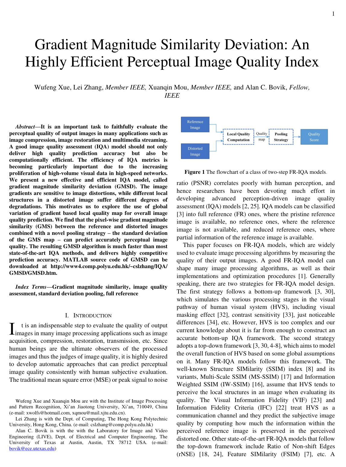
    1. Local quality computation via gradient magnitude similarity (GMS): Given a pristine reference image rr and a distorted image dd, image gradients along orthogonal directions are computed using 3×33 \times 3 Prewitt filters. The pixel-wise gradient magnitude similarity is calculated to form a local quality map (LQM) that captures structural distortions such as blur, additive noise, and compression artifacts.

    2. Global standard deviation (SD) pooling: Rather than taking the spatial average of local quality values (which assumes that all image regions contribute uniformly to perceptual quality), GMSD computes the standard deviation of the GMS map across all pixel locations.

    Because natural images exhibit diverse local structures (such as edges, textures, and smooth regions), different areas experience different degradations under distortion (e.g., blur degrades textured regions more heavily, whereas compression blocking is more visible in flat regions). The standard deviation of the GMS map quantifies the global variation or spread of local quality degradation. A higher GMSD score indicates a wider range of distortion severities across the image and corresponds to lower perceived image quality.

  2. Knowl 2 — Gradient Magnitude Similarity (GMS) Local Quality Map

    equation

    For a reference image rr and a distorted image dd, directional gradients along horizontal (xx) and vertical (yy) directions are computed by convolving the images with 3×33 \times 3 Prewitt filters:

    hx=[1/30−1/31/30−1/31/30−1/3],hy=[1/31/31/3000−1/3−1/3−1/3]h_x = \begin{bmatrix} 1/3 & 0 & -1/3 \\ 1/3 & 0 & -1/3 \\ 1/3 & 0 & -1/3 \end{bmatrix}, \quad h_y = \begin{bmatrix} 1/3 & 1/3 & 1/3 \\ 0 & 0 & 0 \\ -1/3 & -1/3 & -1/3 \end{bmatrix}

    The gradient magnitude maps mr(i)m_r(i) and md(i)m_d(i) at pixel location ii are given by:

    mr(i)=(r⊗hx)2(i)+(r⊗hy)2(i)m_r(i) = \sqrt{(r \otimes h_x)^2(i) + (r \otimes h_y)^2(i)}

    md(i)=(d⊗hx)2(i)+(d⊗hy)2(i)m_d(i) = \sqrt{(d \otimes h_x)^2(i) + (d \otimes h_y)^2(i)}

    where ⊗\otimes denotes the 2D discrete convolution operator.

    The Gradient Magnitude Similarity (GMSGMS) map at pixel ii is defined as:

    GMS(i)=2mr(i)md(i)+cmr(i)2+md(i)2+cGMS(i) = \frac{2 m_r(i) m_d(i) + c}{m_r(i)^2 + m_d(i)^2 + c}

    where c>0c > 0 is a positive constant that ensures numerical stability and mediates contrast response in low-gradient regions. For 8-bit image luminance values normalized to the interval [0,1][0, 1], the constant is set to c=0.0026c = 0.0026. The similarity GMS(i)GMS(i) achieves its maximum value of 11 when mr(i)=md(i)m_r(i) = m_d(i).

  3. Knowl 3 — Standard Deviation Pooling for Image Quality Assessment

    equation

    Given an image containing NN pixels and its pixel-wise Gradient Magnitude Similarity map GMS(i)GMS(i) for i∈{1,…,N}i \in \{1, \dots, N\}, the Gradient Magnitude Similarity Mean (GMSMGMSM) and Gradient Magnitude Similarity Deviation (GMSDGMSD) are defined as:

    GMSM=1N∑i=1NGMS(i)GMSM = \frac{1}{N} \sum_{i=1}^N GMS(i)

    GMSD=1N∑i=1N(GMS(i)−GMSM)2GMSD = \sqrt{\frac{1}{N} \sum_{i=1}^N \left(GMS(i) - GMSM\right)^2}

    GMSMGMSM represents average pooling over the similarity map, functioning as a quality index where larger values reflect superior quality. In contrast, GMSDGMSD measures the standard deviation (spatial variance) of local degradations across different image structures. GMSDGMSD acts as a distortion index where smaller values reflect higher perceptual quality.

  4. Knowl 4 — The Gradient Magnitude Similarity Deviation (GMSD) Algorithm

    algorithm

    The GMSD algorithm evaluates the perceptual quality of a distorted image dd relative to a reference image rr. The inputs are the luminance components of rr and dd, with pixel values normalized to [0,1][0, 1], and a numerical stability parameter c=0.0026c = 0.0026.

    Input: Reference image rr, distorted image dd, stability parameter c=0.0026c = 0.0026
    Output: Distortion index GMSDGMSD
    1. Normalize pixel intensities of rr and dd to the range [0,1][0, 1].
    2. Filter rr and dd with a 2×22 \times 2 average filter, then downsample both images by a factor of 2.
    3. Compute directional gradient images via 2D convolution with Prewitt filters:
       hx=13[10−110−110−1],hy=13[111000−1−1−1]h_x = \frac{1}{3} \begin{bmatrix} 1 & 0 & -1 \\ 1 & 0 & -1 \\ 1 & 0 & -1 \end{bmatrix}, \quad h_y = \frac{1}{3} \begin{bmatrix} 1 & 1 & 1 \\ 0 & 0 & 0 \\ -1 & -1 & -1 \end{bmatrix}
       gr,x=r⊗hx,gr,y=r⊗hyg_{r,x} = r \otimes h_x, \quad g_{r,y} = r \otimes h_y
       gd,x=d⊗hx,gd,y=d⊗hyg_{d,x} = d \otimes h_x, \quad g_{d,y} = d \otimes h_y
    4. Compute gradient magnitude maps at each pixel i∈{1,…,N}i \in \{1, \dots, N\}:
       mr(i)=gr,x(i)2+gr,y(i)2m_r(i) = \sqrt{g_{r,x}(i)^2 + g_{r,y}(i)^2}
       md(i)=gd,x(i)2+gd,y(i)2m_d(i) = \sqrt{g_{d,x}(i)^2 + g_{d,y}(i)^2}
    5. Compute the Gradient Magnitude Similarity map at each pixel ii:
       GMS(i)=2mr(i)md(i)+cmr(i)2+md(i)2+cGMS(i) = \frac{2 m_r(i) m_d(i) + c}{m_r(i)^2 + m_d(i)^2 + c}
    6. Compute the mean similarity score:
       GMSM=1N∑i=1NGMS(i)GMSM = \frac{1}{N} \sum_{i=1}^N GMS(i)
    7. Compute the standard deviation of the GMS map:
       GMSD=1N∑i=1N(GMS(i)−GMSM)2GMSD = \sqrt{\frac{1}{N} \sum_{i=1}^N (GMS(i) - GMSM)^2}
    8. return GMSDGMSD

    The algorithm operates with O(N)O(N) computational time and O(N)O(N) memory storage complexities, requiring 19N19N multiplications and 16N16N additions for an image with NN downsampled pixels.

  5. Knowl 5 — Benchmark Performance Comparison Across Standard IQA Databases

    data/table

    Performance comparison of full-reference image quality assessment (FR-IQA) models evaluated on the LIVE (779 images), CSIQ (886 images), and TID2008 (1700 images) databases. Evaluation metrics include the Spearman Rank-order Correlation Coefficient (SRC) to gauge prediction monotonicity, Pearson linear Correlation Coefficient (PCC) after 5-parameter nonlinear logistic regression to evaluate prediction accuracy, and Root Mean Square Error (RMSE) to assess prediction consistency. The database-weighted average computes overall SRC and PCC weighted by the image count of each database.

    IQA Model LIVE (779 images) CSIQ (886 images) TID2008 (1700 images) Weighted Average
    SRC PCC RMSE SRC PCC RMSE SRC PCC RMSE SRC PCC
    PSNR 0.876 0.872 13.36 0.806 0.751 0.173 0.553 0.523 1.144 0.694 0.664
    IFC 0.926 0.927 10.26 0.767 0.837 0.144 0.568 0.203 1.314 0.703 0.537
    GSD 0.908 0.913 11.149 0.854 0.854 0.137 0.657 0.707 0.949 0.766 0.793
    G-SSIM 0.918 0.920 10.74 0.872 0.874 0.127 0.731 0.760 0.873 0.811 0.827
    SSIM 0.948 0.945 8.95 0.876 0.861 0.133 0.775 0.773 0.851 0.841 0.836
    VIF 0.964 0.960 7.61 0.919 0.928 0.098 0.749 0.808 0.790 0.844 0.875
    MAD 0.944 0.939 9.37 0.899 0.820 0.150 0.771 0.748 0.891 0.845 0.811
    MS-SSIM 0.952 0.950 8.56 0.877 0.659 0.197 0.809 0.801 0.803 0.860 0.798
    GS 0.956 0.951 8.43 0.911 0.896 0.116 0.850 0.842 0.723 0.891 0.882
    GMSM 0.960 0.956 8.049 0.929 0.913 0.107 0.848 0.837 0.735 0.895 0.884
    IW-SSIM 0.957 0.952 8.35 0.921 0.914 0.106 0.856 0.858 0.689 0.896 0.895
    FSIM 0.963 0.960 7.67 0.924 0.912 0.108 0.880 0.874 0.653 0.911 0.904
    GMSD 0.960 0.960 7.62 0.957 0.954 0.079 0.891 0.879 0.640 0.924 0.917

    GMSD achieves the highest overall performance among all tested models across the three databases, delivering the top weighted average SRC (0.9240.924) and PCC (0.9170.917). It outperforms all models on CSIQ and TID2008, while remaining statistically on par with VIF and FSIM on LIVE. The comparison between GMSM (average pooling) and GMSD (standard deviation pooling) demonstrates that standard deviation pooling yields substantial accuracy gains on the gradient magnitude similarity map.

  6. Knowl 6 — Computational Complexity and Running Time Comparison

    data/table

    For an image of NN pixels, computing GMSD requires 2D convolution with two 3×33 \times 3 integer template Prewitt filters, gradient magnitude calculation, pixel-wise GMS computation, and standard deviation pooling. This totals 19N19N multiplications and 16N16N additions, with peak memory storage limited to four directional gradient images of size NN, yielding O(N)O(N) time and memory complexity.

    The execution time of 13 FR-IQA models on a 512×512512 \times 512 image was benchmarked using MATLAB R2010a on a laptop equipped with an Intel Core i7-2600M CPU @ 2.7 GHz and 4 GB RAM:

    Model Running Time (s)
    MAD 2.0715
    IFC 1.1811
    VIF 1.1745
    FSIM 0.5269
    IW-SSIM 0.5196
    MS-SSIM 0.1379
    GS 0.0899
    GSD 0.0481
    SSIM 0.0388
    G-SSIM 0.0379
    GMSD 0.0110
    GMSM 0.0079
    PSNR 0.0016

    GMSD runs in 0.01100.0110 seconds per 512×512512 \times 512 image, executing 3.5×3.5\times faster than SSIM (0.03880.0388 s), 47.9×47.9\times faster than FSIM (0.52690.5269 s), and 106.7×106.7\times faster than VIF (1.17451.1745 s).

  7. Knowl 7 — Effect of Standard Deviation Pooling on Alternative IQA Metrics

    data/table

    Standard deviation (SD) pooling was substituted for the nominal pooling strategies (average pooling or weighted pooling) across six representative FR-IQA models on the LIVE, CSIQ, and TID2008 databases to evaluate whether SD pooling generalizes to other local quality maps (LQMs):

    Model (Weighted) Average Pooling (SRC) SD Pooling (SRC) Performance Gain (%)
    LIVE CSIQ TID2008 LIVE CSIQ TID2008 LIVE CSIQ TID2008
    MSE 0.876 0.806 0.553 0.877 0.834 0.580 +0.18% +3.55% +4.88%
    SSIM 0.948 0.876 0.775 0.917 0.817 0.756 -3.22% -6.71% -2.44%
    MS-SSIM 0.952 0.877 0.809 0.921 0.826 0.650 -3.28% -5.86% -19.71%
    FSIM 0.963 0.924 0.880 0.960 0.956 0.892 -0.33% +3.52% +1.26%
    G-SSIM 0.918 0.872 0.731 0.763 0.757 0.708 -16.93% -13.20% -3.09%
    GSD 0.914 0.828 0.576 0.669 0.611 0.568 -26.76% -26.20% -1.36%

    Except for MSE (which uses single-domain pixel intensity differences) and FSIM on CSIQ/TID2008, SD pooling degraded prediction performance across SSIM, MS-SSIM, G-SSIM, and GSD. This indicates that SD pooling succeeds primarily when the local quality map is computed from a single, homogeneous feature domain (such as gradient magnitude in GMSD or pixel intensity in MSE), whereas combining multiple diverse features (e.g., luminance, contrast, orientation, and structure) introduces complex cross-feature interactions that render the spatial standard deviation uninformative.

  8. Knowl 8 — Cross-Distortion Robustness and Statistical Significance of GMSD

    empirical result

    Statistical hypothesis testing using a left-tailed FF-test at a significance level of 0.050.05 on the nonlinear regression prediction residuals demonstrates that GMSD is statistically superior to competing FR-IQA models:

    1. On LIVE, GMSD is statistically superior to all models except VIF, FSIM, and GMSM (with which it exhibits no statistically significant difference).
    2. On CSIQ, GMSD is statistically superior to all competing models.
    3. On TID2008, GMSD is statistically superior to all models except FSIM.
    4. Across all three benchmark databases, no competing IQA model performs statistically better than GMSD.

    When evaluated on individual distortion types across 28 separate distortion sub-groups across the LIVE, CSIQ, and TID2008 databases, GMSD ranks among the top three models in 14 of the 28 groups (compared to 11 for GS, 10 for VIF, and 8 for PSNR). Unlike models that exhibit divergent regression curves for different distortion categories (such as contrast decrements versus pink Gaussian noise), GMSD yields consistent score distributions across varied distortion families.

  9. Knowl 9 — Five-Parameter Logistic Regression for Objective-to-Subjective Quality Score Mapping

    equation

    To evaluate FR-IQA objective scores against subjective human ratings while accounting for non-linear compression in subjective scoring scales, raw objective quality scores QQ are mapped to nonlinearly fitted scores QpQ_p using a monotonic five-parameter logistic function:

    Qp=β1(12−11+exp⁡(β2(Q−β3)))+β4Q+β5Q_p = \beta_1 \left( \frac{1}{2} - \frac{1}{1 + \exp\left(\beta_2 (Q - \beta_3)\right)} \right) + \beta_4 Q + \beta_5

    where β1,β2,β3,β4,β5∈R\beta_1, \beta_2, \beta_3, \beta_4, \beta_5 \in \mathbb{R} are regression model parameters determined via non-linear least-squares optimization against subjective rating scores SS (such as MOS or DMOS).

    Linear prediction accuracy (Pearson linear Correlation Coefficient, PCC) and prediction consistency (Root Mean Square Error, RMSE) are computed between QpQ_p and SS:

    PCC(Qp,S)=QˉpTSˉQˉpTQˉpSˉTSˉPCC(Q_p, S) = \frac{\bar{Q}_p^T \bar{S}}{\sqrt{\bar{Q}_p^T \bar{Q}_p \bar{S}^T \bar{S}}}

    RMSE(Qp,S)=1n(Qp−S)T(Qp−S)RMSE(Q_p, S) = \sqrt{\frac{1}{n} (Q_p - S)^T (Q_p - S)}

    where Qˉp\bar{Q}_p and Sˉ\bar{S} are the zero-mean versions of QpQ_p and SS, and nn is the total number of images. Prediction monotonicity (Spearman Rank-order Correlation Coefficient, SRC) is rank-based and invariant to monotonic mapping, computed directly between raw scores QQ and SS.

Coverage note — No substantial contributed material was omitted.

References

  1. 1.Z. Wang, “Applications of objective image quality assessment methods,” IEEE Signal Processing Magazine, vol. 28, no. 6, pp. 137 –142, Nov. 2011.
  2. 2.B. Girod, “What's wrong with mean-squared error?” Digital Images and Human Vision. MIT press, 1993.
  3. 3.Z. Wang, and A. C. Bovik, “Modern Image Quality Assessment,” Synthesis Lectures on Image, Video, and Multimedia Processing, vol. 2, no.1, pp. 1-156, 2006.
  4. 4.D. O. Kim, H. S. Han, and R. H. Park, “Gradient information-based image quality metric,” IEEE Transactions on Consumer Electronics, vol. 56, no. 2, pp. 930-936, 2010.
  5. 5.G. Q. Cheng, J. C. Huang, C. Zhu, Z. Liu and L. Z. Cheng, “Perceptual image quality assessment using a geometric structural distortion model,” 17th IEEE International Conference on Image Processing, 2010.
  6. 6.G. H. Chen, C. L. Yang and S. L. Xie, “Gradient-based structural similarity for image quality assessment,” 13th IEEE International Conference on Image Processing, 2006.
  7. 7.Lin Zhang, Lei Zhang, X. Mou and D. Zhang, “FSIM: A Feature Similarity Index for Image Quality Assessment,” IEEE Trans. Image Process., vol. 20, no. 8, pp. 2378-2386, Aug. 2011.
  8. 8.Z. Wang, A C. Bovik and H. R. Sheikh, and E. P. Simoncelli, “Image quality assessment: from error visibility to structural similarity,” IEEE Trans. Image Process., vol. 13, no. 4, pp. 600-612, 2004.
  9. 9.Z. Wang and X. Shang, “Spatial pooling strategies for perceptual image quality assessment,” IEEE Int. Conf. Image Process., Sep. 2006, pp. 2945–2948.
  10. 10.A.K. Moorthy and A.C. Bovik, “Visual importance pooling for image quality assessment,” IEEE J. Special Topics Signal Process, vol. 3, pp. 193-201, April 2009.
  11. 11.H. R. Sheikh, Z. Wang, L. Cormack, and A. C. Bovik. (2005) “Live Image Quality Assessment Database Release 2,” [Online]. http://live.ece.utexas.edu/research/quality.
  12. 12.Eric C. Larson and Damon M. Chandler, “Most apparent distortion: full-reference image quality assessment and the role of strategy,” J. Electron. Imaging 19, 011006, Jan 07, 2010.
  13. 13.N. Ponomarenko, V. Lukin, A. Zelensky, K. Egiazarian, M. Carli, F. Battisti, “TID2008 - A Database for Evaluation of Full-Reference Visual Quality Assessment Metrics,” Advances of Modern Radio electronics, Vol. 10, pp. 30-45, 2009.
  14. 14.Lin Zhang, Lei Zhang, X. Mou and D. Zhang, “A Comprehensive Evaluation of Full Reference Image Quality Assessment Algorithms,” IEEE Int. Conf. Image Process. 2012.
  15. 15.A. Liu, W. Lin, and Manish Narwaria, “Image Quality Assessment Based on Gradient Similarity,” IEEE Transactions on Image Processing, vol. 21, no. 4, pp. 1500-1512, 2012.
  16. 16.Z. Wang, and Q. Li, “Information content weighting for perceptual image quality assessment,” IEEE Transactions on Image Processing, vol. 20, no. 5, pp. 1185-1198, 2011.
  17. 17.Z. Wang, E. P. Simoncelli, and A. C. Bovik, “Multiscale structural similarity for image quality assessment,” Conference Record of the Thirty-Seventh Asilomar Conference on Signals, Systems and Computers, vol. 2, IEEE, 2003.
  18. 18.M. Zhang, X. Mou, and L. Zhang, “Non-Shift Edge Based Ratio (NSER): An Image Quality Assessment Metric Based on Early Vision Features,” IEEE Signal Processing Letters, vol. 18, no .5, pp. 315-318, 2011.
  19. 19.C. F. Li, and A. C. Bovik, “Content-partitioned structural similarity index for image quality assessment,” Signal Processing: Image Communication, vol. 25, no. 7, pp. 517-526, 2010.
  20. 20.Y. Tong, Hubert Konik, F. A. Cheikh and Alain Tremeau, “Full reference image quality assessment based on saliency map analysis,” Journal of Imaging Science, vol. 54, no. 3, pp. 30503-30503, 2010.
  21. 21.VQEG, “Final report from the Video Quality Experts Group on the validation of objective models of video quality assessment – Phase II,” August 2003, available at http://www.vqeg.org/.
  22. 22.H.R. Sheikh, A.C. Bovik and G. de Veciana, “An information fidelity criterion for image quality assessment using natural scene statistics,” IEEE Transactions on Image Processing, vol.14, no.12pp. 2117- 2128, Dec. 2005.
  23. 23.H.R. Sheikh, and A.C. Bovik, “Image information and visual quality,” IEEE Transactions on Image Processing, vol.15, no.2, pp. 430- 444, Feb. 2006.
  24. 24.W. Xue, and X. Mou, “An image quality assessment metric based on Non-shift Edge,” 18th IEEE International Conference on Image Processing (ICIP), 2011.
  25. 25.Z. Wang and A. C. Bovik, “Mean squared error: love it or leave it? - A new look at signal fidelity measures,” IEEE Signal Processing Magazine, vol. 26, no. 1, pp. 98-117, Jan. 2009.
  26. 26.A.L. Neuenschwander, M.M. Crawford, L.A. Magruder, C. A. Weed, R. Cannata, D. Fried, R. Knowlton and R. Heinrichs, “Classification of LADAR data over Haitian urban environments using a lower envelope follower and adaptive gradient operator,” Proc. SPIE 7684, 768408 (2010).
  27. 27.S. A. Coleman, B. W. Scotney, and S. Suganthan, “Multi-scale edge detection on range and intensity images,” Pattern Recognition, vol. 44, no. 4, pp. 821-838, 2011.
  28. 28.Nezhadarya Ehsan, and Rabab K. Ward, “An efficient method for robust gradient estimation of RGB color images,” 16th IEEE International Conference on Image Processing (ICIP), 2009.
  29. 29.J. Park, K. Seshadrinathan, S. Lee and A.C. Bovik, “VQpooling: Video quality pooling adaptive to perceptual distortion severity,” IEEE Transactions on Image Processing, vol. 22, no. 2, pp. 610-620, February 2013.
  30. 30.W. Lin, C.-C. Jay Kuo, “Perceptual visual quality metrics: A survey,” Journal of Visual Communication and Image Representation, vol. 22, no. 4, pp. 297-312, May 2011.
  31. 31.Ninassi, Alexandre, et al., “Does where you gaze on an image affect your perception of quality? Applying visual attention to image quality metric,” IEEE International Conference on Image Processing, vol. 2, 2007.
  32. 32.J. Ross and H. D. Speed, “Contrast adaptation and contrast masking in human vision,” Proceedings. Biological Sciences / The Royal Society, vol. 246, no. 1315, pp. 61–9, Oct. 1991.
  33. 33.S. J. Daly, “Application of a noise-adaptive contrast sensitivity function to image data compression,” Optical Engineering, vol. 29, pp. 977–987, 1990.
  34. 34.Lubin, Jeffrey. “A human vision system model for objective picture quality measurements,” International Broadcasting Conference (IBC), January 1997 p. 498 – 503.
  35. 35.Carlos M. Jarque, Anil K. Bera, “Efficient tests for normality, homoscedasticity and serial independence of regression residuals,” Economics Letters 6 (3): 255–259, 1980.
  36. 36.Chao Wang, Xuanqin Mou, Wei Hong, and Lei Zhang, “Block-layer bit allocation for quality constrained video encoding based on constant perceptual quality,” Proceedings of SPIE Vol. 8666, 86660J (2013).
  37. 37.Tao-Sheng Ou, Yi-Hsin Huang, and Homer H. Chen, “SSIM-based perceptual rate control for video coding," IEEE Transactions on Circuits and Systems for Video Technology, vol. 21, no. 5, pp. 682-691, 2011.
  38. 38.Shiqi Wang, Abdul Rehman, Z. Wang, Siwei Ma, and Wen Gao, “SSIM-motivated rate-distortion optimization for video coding,” IEEE Transactions on Circuits and Systems for Video Technology, vol. 22, no. 4 (2012): 516-529.
  39. 39.Z. Wang, A. C. Bovik and H. R. Sheikh, and E. P. Simoncelli, “The SSIM index for image quality assessment,” MATLAB implementation available online from: http://www.cns.nyu.edu/lcv/ssim/ssim.m.
  40. 40.D. Jayaraman, A. Mittal, A. K. Moorthy and A. C. Bovik, “LIVE Multiply Distorted Image Quality Database,” online at: http://live.ece.utexas.edu/research/quality/live_multidistortedimage.html.
  41. 41.A. K. Moorthy, L. K. Choi, A. C. Bovik and G. deVeciana, “Video Quality Assessment on Mobile Devices: Subjective, Behavioral and Objective Studies,” IEEE Journal of Selected Topics in Signal Processing, vol. 6, no. 6, pp. 652-671, October 2012.
  42. 42.Ming-Jun Chen, and A. C. Bovik, “Fast structural similarity index algorithm,” Journal of Real-Time Image Processing, vol. 6, no. 4 (2011): 281-287.
  43. 43.R. Soundararajan and A. C. Bovik, “RRED indices: Reduced reference entropic differencing for image quality assessment,” IEEE Transactions on Image Processing, vol. 21, no. 2, pp. 517-526, Feb. 2012.

Citation

MLA
Xue, W., et al. “Gradient Magnitude Similarity Deviation: A Highly Efficient Perceptual Image Quality Index”. IEEE Transactions on Image Processing, vol. 23, no. 2, 2014, pp. 684–95, https://doi.org/10.1109/TIP.2013.2293423.
APA
Xue, W., Zhang, L., Mou, X., & Bovik, A. C. (2014). Gradient Magnitude Similarity Deviation: A Highly Efficient Perceptual Image Quality Index. IEEE Transactions on Image Processing, 23(2), 684–695. https://doi.org/10.1109/TIP.2013.2293423
Chicago
Xue, W., L. Zhang, X. Mou, and A. C. Bovik. 2014. “Gradient Magnitude Similarity Deviation: A Highly Efficient Perceptual Image Quality Index”. IEEE Transactions on Image Processing 23 (2): 684–95. https://doi.org/10.1109/TIP.2013.2293423.
Harvard
Xue, W. et al. (2014) “Gradient Magnitude Similarity Deviation: A Highly Efficient Perceptual Image Quality Index”, IEEE Transactions on Image Processing, 23(2), pp. 684–695. Available at: https://doi.org/10.1109/TIP.2013.2293423.
Vancouver
1. Xue W, Zhang L, Mou X, Bovik AC (2014) Gradient Magnitude Similarity Deviation: A Highly Efficient Perceptual Image Quality Index. IEEE Transactions on Image Processing 23:684–695

BibTeX

@article{Xue_2014, title={Gradient Magnitude Similarity Deviation: A Highly Efficient Perceptual Image Quality Index}, volume={23}, ISSN={1941-0042}, url={http://dx.doi.org/10.1109/TIP.2013.2293423}, DOI={10.1109/tip.2013.2293423}, number={2}, journal={IEEE Transactions on Image Processing}, publisher={Institute of Electrical and Electronics Engineers (IEEE)}, author={Xue, Wufeng and Zhang, Lei and Mou, Xuanqin and Bovik, Alan C.}, year={2014}, month=Feb, pages={684–695} }
Metadata:Crossref

Access the Paper

This paper is available from its original source. Click below to access the PDF.

Open PDF