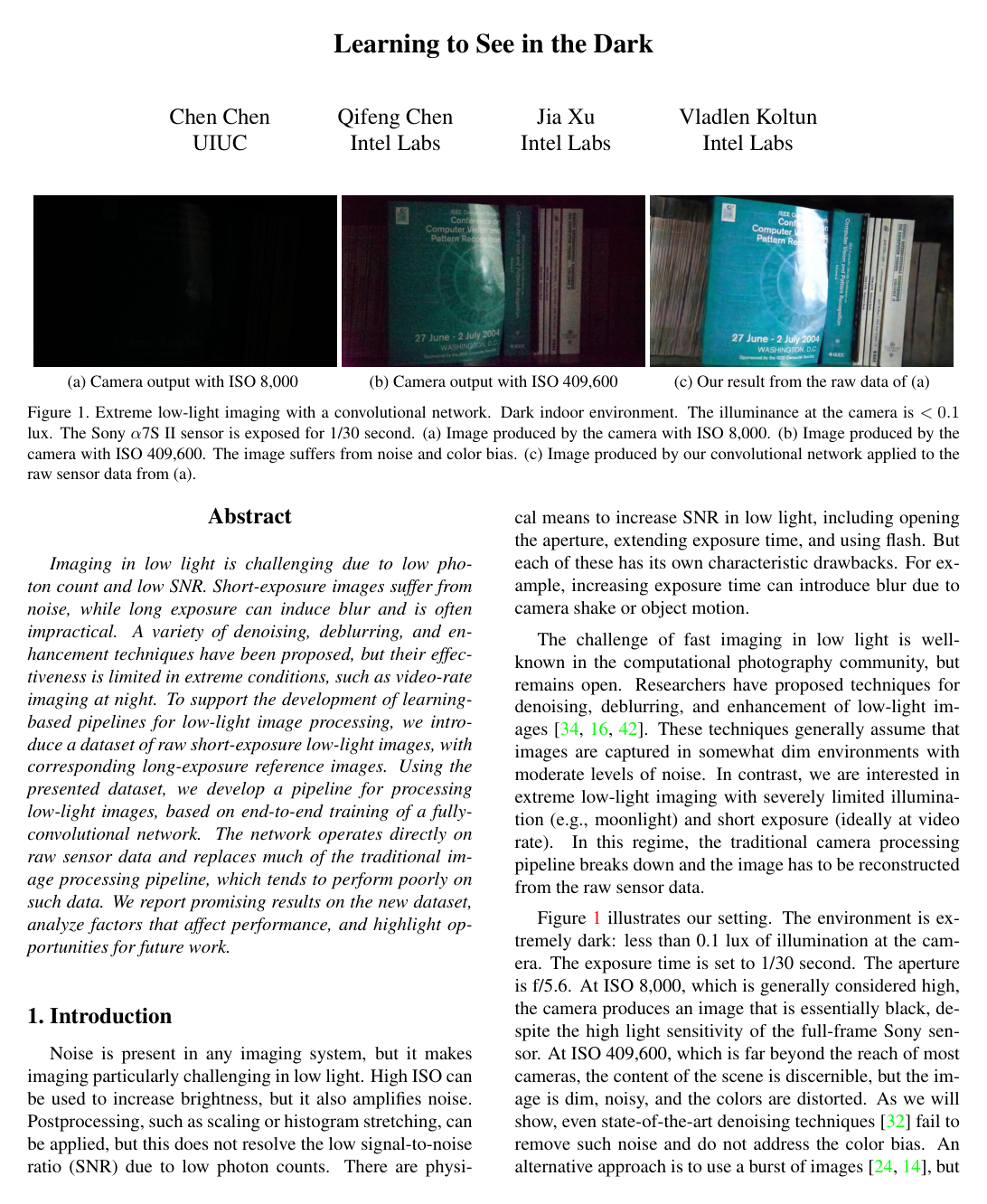
Learning to See in the Dark

Chen ChenQifeng ChenJia XuVladlen Koltun

article2018CVPR1,589 citations

Introduces a raw-sensor low-light image dataset and a fully convolutional network pipeline that replaces traditional camera processing to produce clear, high-signal photographs from extreme short-exposure night shots.

Listen

Capturing clear images in extreme low-light environments, such as illumination levels below 0.1 lux, remains a significant challenge. Short-exposure photos suffer from severe sensor noise and low signal-to-noise ratios, while long exposures often cause motion blur and are impractical for dynamic scenes or video. Traditional camera pipelines and standard denoising tools break down in these conditions because they amplify noise and distort colors rather than recovering true scene details.

The article introduces an end-to-end deep learning framework designed to replace the traditional camera processing pipeline for extreme low-light raw image processing. It demonstrates how a fully-convolutional neural network can directly convert dark, short-exposure raw sensor data into clear, full-color images without the compounding errors of conventional multi-stage processing.

To develop and evaluate this method, the authors collected the See-in-the-Dark dataset, consisting of 5,094 short-exposure raw images matched with 424 corresponding long-exposure reference images captured on Sony and Fujifilm cameras. Using this data, the authors trained a U-Net architecture directly on raw sensor data with an adjustable amplification factor, evaluating the output through both objective image quality metrics and blind human perceptual studies on Amazon Mechanical Turk.

The findings show that the proposed network dramatically outperforms existing methods in extreme low light. In perceptual tests on heavily under-exposed images amplified up to 300 times, human evaluators preferred the neural network's output over the state-of-the-art BM3D denoising baseline in 92.4% of comparisons and over an idealized eight-frame burst-merging baseline in 85.2% of comparisons. Controlled experiments revealed that processing raw sensor data directly was critical, as operating on standard sRGB outputs resulted in severe performance drops. The U-Net architecture also proved superior in color preservation compared to alternative context aggregation architectures, and the model successfully generalized to images from an iPhone 6s despite being trained on a different camera sensor.

These results indicate that data-driven neural pipelines can bypass traditional camera hardware limitations, unlocking viable night-time and sub-lux photography on consumer-grade sensors without requiring bulky auxiliary lighting or multi-image bursts. This shift reduces system complexity while offering substantial performance improvements for computer vision applications operating in poorly lit settings.

Before broad commercial deployment, organizations should pursue several next steps. Engineering efforts should focus on runtime optimization, as full-resolution processing currently takes 0.38 to 0.66 seconds per frame, which is insufficient for real-time video. Further research should also develop automated amplification estimation (akin to Auto ISO) and incorporate dynamic range tone mapping to prevent highlight saturation.

Decision-makers should note that the dataset consists exclusively of static scenes without moving subjects, and extreme amplification factors (such as 300-fold scaling) can still exhibit fine-detail loss. However, confidence remains high that direct neural processing of raw sensor data provides a fundamentally superior baseline for low-light computational imaging compared to traditional multi-step pipelines.

Cover for Learning to See in the Dark

Abstract

Imaging in low light is challenging due to low photon count and low SNR. Short-exposure images suffer from noise, while long exposure can induce blur and is often impractical. A variety of denoising, deblurring, and enhancement techniques have been proposed, but their effectiveness is limited in extreme conditions, such as video-rate imaging at night. To support the development of learning-based pipelines for low-light image processing, we introduce a dataset of raw short-exposure low-light images, with corresponding long-exposure reference images. Using the presented dataset, we develop a pipeline for processing low-light images, based on end-to-end training of a fully-convolutional network. The network operates directly on raw sensor data and replaces much of the traditional image processing pipeline, which tends to perform poorly on such data. We report promising results on the new dataset, analyze factors that affect performance, and highlight opportunities for future work. The results are shown in the supplementary video at this https URL

Table of Contents

  • 1. Introduction
  • 2. Related Work
  • 3. See-in-the-Dark Dataset
  • 4. Method
  • 4.1. Pipeline
  • 4.2. Training
  • 5. Experiments
  • 5.1. Qualitative results and perceptual experiments
  • 5.2. Controlled experiments
  • 6. Discussion
  • References

Knowls

  1. Knowl 1 — End-to-End Raw Image Processing Pipeline for Extreme Low-Light Imaging

    model/method

    The See-in-the-Dark (SID) pipeline replaces the traditional camera image signal processor (ISP)—which sequentially applies white balancing, demosaicing, denoising, sharpening, color space conversion, and gamma correction—with a single fully-convolutional network (FCN).

    Given a single short-exposure raw sensor image with height HH and width WW:

    1. Packing: A 1-channel raw Bayer image of size H×W×1H \times W \times 1 is packed into a 4-channel tensor of size H2×W2×4\frac{H}{2} \times \frac{W}{2} \times 4. For X-Trans sensors (6×66 \times 6 pattern), raw pixels are rearranged into a 9-channel tensor of size H3×W3×9\frac{H}{3} \times \frac{W}{3} \times 9.
    2. Amplification and Bias Subtraction: The sensor black level BblackB_{\text{black}} is subtracted, and the tensor is scaled by an external amplification ratio α\alpha (e.g., ×100\times 100, ×250\times 250, or ×300\times 300), analogous to camera ISO: X=α⋅(Xpacked−Bblack)X = \alpha \cdot (X_{\text{packed}} - B_{\text{black}})
    3. Feature Processing: The scaled tensor XX is fed into a U-Net convolutional architecture. The network outputs a 12-channel feature map of size H2×W2×12\frac{H}{2} \times \frac{W}{2} \times 12.
    4. Resolution Recovery: A sub-pixel convolutional layer (pixel shuffle) rearranges the 12 half-resolution channels into a full-resolution 3-channel RGB image in sRGB color space of dimensions H×W×3H \times W \times 3.

    The entire network performs joint denoising, demosaicing, color correction, and tone adjustment blindly without separate pipeline stages.

  2. Knowl 2 — See-in-the-Dark (SID) Dataset

    experimental setup

    The See-in-the-Dark (SID) dataset contains 5,094 raw short-exposure low-light images paired with 424 unique long-exposure reference images for training and evaluation:

    • Illumination Levels: Outdoor nighttime scenes (moonlight or street lighting) range from 0.2 to 5.0 lux at the camera. Indoor scenes in dark rooms with faint indirect illumination range from 0.03 to 0.3 lux.
    • Exposure Ratios: Short input exposures range from 1/30 s1/30\text{ s} to 1/10 s1/10\text{ s}. Reference images were captured with 100 to 300 times longer exposure durations (10 s10\text{ s} to 30 s30\text{ s}).
    • Sensors and Resolutions:
      1. Sony α\alpha7S II: Full-frame Bayer CFA, 4240×28324240 \times 2832 resolution. Contains 1,190 images at ×300\times 300 exposure ratio, 699 images at ×250\times 250, and 808 images at ×100\times 100.
      2. Fujifilm X-T2: APS-C X-Trans CFA, 6000×40006000 \times 4000 resolution. Contains 630 images at ×300\times 300 exposure ratio, 650 images at ×250\times 250, and 1,117 images at ×100\times 100.
    • Capture Protocol: Mirrorless cameras were mounted on sturdy tripods to prevent camera shake across static scenes. Reference images were processed into sRGB ground truths using LibRaw. The dataset is partitioned into 70% training, 10% validation, and 20% test splits per condition.
  3. Knowl 3 — Controlled Experiments on Network Architecture, Loss Functions, and Data Encodings

    data/table

    Controlled experiments evaluate different pipeline configurations using Peak Signal-to-Noise Ratio (PSNR in dB) and Structural Similarity (SSIM):

    Condition Sony (PSNR / SSIM) Fuji (PSNR / SSIM)
    Default pipeline (U-Net, Raw, L1L_1, Packed) 28.88 / 0.787 26.61 / 0.680
    Network: U-Net →\to CAN 27.40 / 0.792 25.71 / 0.710
    Input color space: Raw →\to sRGB 17.40 / 0.554 25.11 / 0.648
    Loss function: L1→L_1 \to SSIM loss 28.64 / 0.817 26.20 / 0.685
    Loss function: L1→L2L_1 \to L_2 loss 28.47 / 0.784 26.51 / 0.680
    Data arrangement: Packed →\to Masked 26.95 / 0.744 –
    X-Trans packing: 3×3→6×63 \times 3 \to 6 \times 6 – 23.05 / 0.567
    Reference targets: Stretched references 18.23 / 0.674 16.85 / 0.535

    Key empirical findings:

    • Architecture: U-Net achieves higher PSNR than the multi-scale Context Aggregation Network (CAN) on both sensors. While CAN achieves slightly higher SSIM, it suffers from severe desaturation and loss of color.
    • Loss Functions: L1L_1, L2L_2, and SSIM loss yield comparable accuracy without noticeable perceptual differences. Total variation regularizers yield no improvement, and generative adversarial network (GAN) losses degrade accuracy.
    • Data Arrangement: Packing Bayer data into 4 channels outperforms 1-channel spatial masking (28.88 vs. 26.95 dB). For X-Trans sensors, 3×33 \times 3 packing into 9 channels outperforms 6×66 \times 6 packing into 36 channels (26.61 vs. 23.05 dB).
  4. Knowl 4 — End-to-End Raw Training Algorithm for Low-Light Enhancement

    algorithm

    The network is trained from scratch per camera sensor using raw short-exposure inputs and corresponding LibRaw-converted long-exposure sRGB reference images.

    Input: Dataset of pairs (Xraw(i),Yraw(i)X_{\text{raw}}^{(i)}, Y_{\text{raw}}^{(i)}), exposure ratios α(i)=tref(i)/tin(i)\alpha^{(i)} = t_{\text{ref}}^{(i)} / t_{\text{in}}^{(i)}, black level BblackB_{\text{black}}
    Output: Trained convolutional network parameters θ\theta
    Initialize network weights θ\theta
    Generate sRGB ground truth images YsRGB(i)←LibRaw(Yraw(i))Y_{\text{sRGB}}^{(i)} \leftarrow \text{LibRaw}(Y_{\text{raw}}^{(i)})
    Set initial learning rate η←10−4\eta \leftarrow 10^{-4}
    for epoch = 1 to 4000 do
        if epoch = 2001 then
            η←10−5\eta \leftarrow 10^{-5}
        for each batch of training pairs do
            Extract random 512×512512 \times 512 patches from XrawX_{\text{raw}} and YsRGBY_{\text{sRGB}}
            Apply random horizontal flip, vertical flip, and 90∘90^\circ rotation
            Xpacked←PackRaw(Xraw)X_{\text{packed}} \leftarrow \text{PackRaw}(X_{\text{raw}})
            Xin←α⋅(Xpacked−Bblack)X_{\text{in}} \leftarrow \alpha \cdot (X_{\text{packed}} - B_{\text{black}})
            Y^←fθ(Xin)\hat{Y} \leftarrow f_\theta(X_{\text{in}})
            L1←1∣P∣∑p∈P∣Y^p−YsRGB,p∣\mathcal{L}_1 \leftarrow \frac{1}{|P|} \sum_{p \in P} |\hat{Y}_p - Y_{\text{sRGB}, p}|
            Update θ\theta using Adam optimizer with gradient ∇θL1\nabla_\theta \mathcal{L}_1 and learning rate η\eta
    return θ\theta
  5. Knowl 5 — Blind Perceptual Evaluation Against BM3D and Burst Denoising

    data/table

    A blind randomized A/B perceptual experiment on Amazon Mechanical Turk compared the proposed single-image pipeline against two baselines:

    1. BM3D: 3D transform-domain collaborative filtering applied post-hoc to the amplified output of the standard camera pipeline.
    2. Burst Denoising: Pixel-wise median aggregation across 8 consecutively captured, perfectly aligned short-exposure raw images.

    To ensure fair comparison despite different image pipelines, baseline outputs received privileged oracle adjustments: white-balance coefficients extracted from reference images and channel-wise mean scaling matching the ground truth.

    Comparison Sony ×300\times 300 Set (Challenging) Sony ×100\times 100 Set (Easier)
    Ours >> BM3D 92.4% 59.3%
    Ours >> Burst (8 images) 85.2% 47.3%

    A total of 1,180 pairwise comparisons were evaluated across 10 workers. On the extreme low-light imes300 imes 300 subset (under 0.1 lux), the single-image neural pipeline was preferred over BM3D in 92.4% of comparisons and over 8-frame burst denoising in 85.2% of comparisons. On the imes100 imes 100 subset, the single-image model performed comparably to 8-frame burst aggregation (47.3%) while outperforming BM3D (59.3%).

  6. Knowl 6 — Impact of Raw vs. sRGB Input Domain on Extreme Low-Light Reconstruction

    empirical result

    Feeding raw sensor data directly into the neural network significantly outperforms training the network on sRGB images produced by a traditional camera processing pipeline:

    • On the Sony dataset, raw input processing achieves a PSNR of 28.88 dB and SSIM of 0.787, whereas applying the network to sRGB pipeline outputs yields a PSNR of 17.40 dB and SSIM of 0.554 (an 11.48 dB degradation).
    • On the Fujifilm dataset, raw input processing achieves 26.61 dB PSNR / 0.680 SSIM compared to 25.11 dB PSNR / 0.648 SSIM on sRGB inputs.

    In extreme low-light environments, traditional camera ISP stages (white balance, non-linear gamma, and quantization) amplify shot and read noise while irreversibly clipping pixel intensities into narrow, distorted dynamic ranges. Operating directly on linear raw sensor data preserves high-bit-depth signal distributions and allows the convolutional network to perform noise suppression before non-linear distortions accumulate.

  7. Knowl 7 — Color Filter Array Channel Packing for Bayer and X-Trans Sensors

    model/method

    To feed single-channel color filter array (CFA) raw data into standard convolutional layers without introducing spatial sparsity:

    • Bayer CFA Packing: Bayer raw data of size H×W×1H \times W \times 1 (consisting of 2×22 \times 2 sub-patterns: R, G, G, B) is packed into 4 channels of dimensions H2×W2×4\frac{H}{2} \times \frac{W}{2} \times 4. Compared to masking/padding zeros into 3 full-size channels, packing prevents sparse convolution artifacts, avoids hue distortion, and improves PSNR from 26.95 dB to 28.88 dB.
    • X-Trans CFA Packing: The Fujifilm X-Trans mosaic has a repeating 6×66 \times 6 block structure. Directly packing this into 36 channels of size H6×W6×36\frac{H}{6} \times \frac{W}{6} \times 36 drops PSNR to 23.05 dB and causes loss of fine detail. Instead, adjacent elements are exchanged to form 3×33 \times 3 sub-blocks packed into 9 channels of size H3×W3×9\frac{H}{3} \times \frac{W}{3} \times 9, yielding 26.61 dB PSNR.
  8. Knowl 8 — Inability of Fully-Convolutional Networks to Learn Global Histogram Stretching

    empirical result

    When long-exposure reference images are normalized using global histogram stretching during training, forcing the network to simultaneously learn global contrast adjustment alongside demosaicing and denoising:

    • Reconstruction performance drops drastically from 28.88 dB to 18.23 dB PSNR on the Sony dataset and from 26.61 dB to 16.85 dB PSNR on the Fujifilm dataset.
    • Output images exhibit severe spatial splotching and color artifacts across uniform regions (e.g., walls).

    Because standard fully-convolutional networks rely on spatially invariant local operations, they struggle to model and manipulate global whole-image histogram statistics. Attempting to fit global tone curves causes severe overfitting to training scene illuminations. Consequently, global histogram manipulation must be decoupled from the network and applied optionally as post-processing.

  9. Knowl 9 — Cross-Sensor Generalization of Bayer Raw Denoising to Mobile Sensors

    empirical result

    A model trained exclusively on the Sony α\alpha7S II dataset (full-frame Bayer sensor) was evaluated directly on 14-bit raw Bayer images captured by an Apple iPhone 6s in nighttime conditions (0.05 s exposure, f/2.2f/2.2, ISO 400) at an amplification factor of ×100\times 100.

    Without sensor-specific fine-tuning or retraining, the network successfully suppressed extreme sensor noise, corrected color bias, and recovered high scene contrast. This demonstrates that deep networks trained on linear raw Bayer data learn demosaicing and denoising priors that can generalize across different hardware sensors sharing the same Bayer pattern structure.

  10. Knowl 10 — Operational Limitations and Runtime Constraints of the SID Pipeline

    limitation

    The See-in-the-Dark low-light processing pipeline has several operational limitations:

    1. Static Scene Assumption: The dataset and evaluation are restricted to static scenes due to the 10–30 second reference exposure times; dynamic scenes with moving humans or objects are not supported.
    2. External Amplification Factor: The amplification ratio α\alpha must be specified manually as an external parameter rather than being automatically estimated from the input image.
    3. Absence of HDR Tone Mapping: The network outputs directly to standard dynamic range sRGB space, resulting in overexposure and saturation artifacts in bright highlight regions.
    4. Latency and GPU Memory: Inference on full-resolution raw images requires 0.38 seconds for Sony (4240×28324240 \times 2832) and 0.66 seconds for Fuji (6000×40006000 \times 4000) on GPU. This prevents real-time full-resolution video capture (30 fps), although real-time processing is possible at reduced preview resolutions.
    5. Loss of Detail in Extreme Photon Starvation: In sub-0.1 lux settings at ×300\times 300 amplification, signal recovery is constrained by photon counts, resulting in visible smoothing and texture degradation.

Coverage note — None was omitted; all key architectural components, dataset parameters, experimental comparisons, ablations, and stated limitations are fully covered.

References

  1. 1.F. Agostinelli, M. R. Anderson, and H. Lee. Adaptive multicolumn deep neural networks with application to robust image denoising. In NIPS, 2013.
  2. 2.J. Anaya and A. Barbu. RENOIR – A dataset for real lowlight image noise reduction. arXiv:1409.8230, 2014.
  3. 3.H. C. Burger, C. J. Schuler, and S. Harmeling. Image denoising: Can plain neural networks compete with BM3D? In CVPR, 2012.
  4. 4.Q. Chen and V. Koltun. Photographic image synthesis with cascaded refinement networks. In ICCV, 2017.
  5. 5.Q. Chen, J. Xu, and V. Koltun. Fast image processing with fully-convolutional networks. In ICCV, 2017.
  6. 6.Y. Chen and T. Pock. Trainable nonlinear reaction diffusion: A flexible framework for fast and effective image restoration. IEEE Transactions on Pattern Analysis and Machine Intelligence, 39(6), 2017.
  7. 7.K. Dabov, A. Foi, V. Katkovnik, and K. Egiazarian. Image denoising by sparse 3-D transform-domain collaborative filtering. IEEE Transactions on Image Processing, 16(8), 2007.
  8. 8.X. Dong, G. Wang, Y. Pang, W. Li, J. Wen, W. Meng, and Y. Lu. Fast efficient algorithm for enhancement of low lighting video. In IEEE International Conference on Multimedia and Expo, 2011.
  9. 9.M. Elad and M. Aharon. Image denoising via sparse and redundant representations over learned dictionaries. IEEE Transactions on Image Processing, 15(12), 2006.
  10. 10.M. Gharbi, G. Chaurasia, S. Paris, and F. Durand. Deep joint demosaicking and denoising. ACM Transactions on Graphics, 35(6), 2016.
  11. 11.I. Goodfellow, J. Pouget-Abadie, M. Mirza, B. Xu, D. Warde-Farley, S. Ozair, A. Courville, and Y. Bengio. Generative adversarial nets. In NIPS, 2014.
  12. 12.S. Gu, L. Zhang, W. Zuo, and X. Feng. Weighted nuclear norm minimization with application to image denoising. In CVPR, 2014.
  13. 13.X. Guo, Y. Li, and H. Ling. LIME: Low-light image enhancement via illumination map estimation. IEEE Transactions on Image Processing, 26(2), 2017.
  14. 14.S. W. Hasinoff, D. Sharlet, R. Geiss, A. Adams, J. T. Barron, F. Kainz, J. Chen, and M. Levoy. Burst photography for high dynamic range and low-light imaging on mobile cameras. ACM Transactions on Graphics, 35(6), 2016.
  15. 15.K. Hirakawa and T. W. Parks. Joint demosaicing and denoising. IEEE Transactions on Image Processing, 15(8), 2006.
  16. 16.Z. Hu, S. Cho, J. Wang, and M.-H. Yang. Deblurring lowlight images with light streaks. In CVPR, 2014.
  17. 17.V. Jain and H. S. Seung. Natural image denoising with convolutional networks. In NIPS, 2008.
  18. 18.H. Jiang, Q. Tian, J. E. Farrell, and B. A. Wandell. Learning the image processing pipeline. IEEE Transactions on Image Processing, 26(10), 2017.
  19. 19.N. Joshi and M. F. Cohen. Seeing Mt. Rainier: Lucky imaging for multi-image denoising, sharpening, and haze removal. In ICCP, 2010.
  20. 20.J. Kim, J. K. Lee, and K. M. Lee. Accurate image superresolution using very deep convolutional networks. In CVPR, 2016.
  21. 21.D. P. Kingma and J. Ba. Adam: A method for stochastic optimization. In ICLR, 2015.
  22. 22.Y. LeCun, B. Boser, J. S. Denker, D. Henderson, R. E. Howard, W. Hubbard, and L. D. Jackel. Backpropagation applied to handwritten zip code recognition. Neural Computation, 1(4), 1989.
  23. 23.C. Liu and W. T. Freeman. A high-quality video denoising algorithm based on reliable motion estimation. In ECCV, 2010.
  24. 24.Z. Liu, L. Yuan, X. Tang, M. Uyttendaele, and J. Sun. Fast burst images denoising. ACM Transactions on Graphics, 33(6), 2014.
  25. 25.J. Long, E. Shelhamer, and T. Darrell. Fully convolutional networks for semantic segmentation. In CVPR, 2015.
  26. 26.K. G. Lore, A. Akintayo, and S. Sarkar. LLNet: A deep autoencoder approach to natural low-light image enhancement. Pattern Recognition, 61, 2017.
  27. 27.A. Łoza, D. R. Bull, P. R. Hill, and A. M. Achim. Automatic contrast enhancement of low-light images based on local statistics of wavelet coefficients. Digital Signal Processing, 23(6), 2013.
  28. 28.J. Mairal, F. Bach, J. Ponce, G. Sapiro, and A. Zisserman. Non-local sparse models for image restoration. In ICCV, 2009.
  29. 29.H. Malm, M. Oskarsson, E. Warrant, P. Clarberg, J. Hasselgren, and C. Lejdfors. Adaptive enhancement and noise reduction in very low light-level video. In ICCV, 2007.
  30. 30.S. Park, S. Yu, B. Moon, S. Ko, and J. Paik. Low-light image enhancement using variational optimization-based Retinex model. IEEE Transactions on Consumer Electronics, 63(2), 2017.
  31. 31.G. Petschnigg, R. Szeliski, M. Agrawala, M. Cohen, H. Hoppe, and K. Toyama. Digital photography with flash and no-flash image pairs. ACM Transactions on Graphics, 23(3), 2004.
  32. 32.T. Plötz and S. Roth. Benchmarking denoising algorithms with real photographs. In CVPR, 2017.
  33. 33.J. Portilla, V. Strela, M. J. Wainwright, and E. P. Simoncelli. Image denoising using scale mixtures of Gaussians in the wavelet domain. IEEE Transactions on Image Processing, 12(11), 2003.
  34. 34.T. Remez, O. Litany, R. Giryes, and A. M. Bronstein. Deep convolutional denoising of low-light images. arXiv:1701.01687, 2017.
  35. 35.O. Ronneberger, P. Fischer, and T. Brox. U-net: Convolutional networks for biomedical image segmentation. In MICCAI, 2015.
  36. 36.L. I. Rudin, S. Osher, and E. Fatemi. Nonlinear total variation based noise removal algorithms. Physica D: Nonlinear Phenomena, 60(1-4), 1992.
  37. 37.W. Shi, J. Caballero, F. Huszár, J. Totz, A. P. Aitken, R. Bishop, D. Rueckert, and Z. Wang. Real-time single image and video super-resolution using an efficient sub-pixel convolutional neural network. In CVPR, 2016.
  38. 38.Z. Wang, A. C. Bovik, H. R. Sheikh, and E. P. Simoncelli. Image quality assessment: From error visibility to structural similarity. IEEE Transactions on Image Processing, 13(4), 2004.
  39. 39.J. Xie, L. Xu, and E. Chen. Image denoising and inpainting with deep neural networks. In NIPS, 2012.
  40. 40.L. Xu, J. Ren, Q. Yan, R. Liao, and J. Jia. Deep edge-aware filters. In ICML, 2015.
  41. 41.K. Zhang, W. Zuo, Y. Chen, D. Meng, and L. Zhang. Beyond a Gaussian denoiser: Residual learning of deep CNN for image denoising. IEEE Transactions on Image Processing, 26(7), 2017.
  42. 42.X. Zhang, P. Shen, L. Luo, L. Zhang, and J. Song. Enhancement and noise reduction of very low light level images. In ICPR, 2012.
  43. 43.H. Zhao, O. Gallo, I. Frosio, and J. Kautz. Loss functions for image restoration with neural networks. IEEE Transactions on Computational Imaging, 3(1), 2017.

Citation

MLA
Chen, C., et al. “Learning to See in the Dark”. arXiv, 2018, http://arxiv.org/abs/1805.01934v1.
APA
Chen, C., Chen, Q., Xu, J., & Koltun, V. (2018). Learning to See in the Dark. arXiv. http://arxiv.org/abs/1805.01934v1
Chicago
Chen, C., Q. Chen, J. Xu, and V. Koltun. 2018. “Learning to See in the Dark”. arXiv. http://arxiv.org/abs/1805.01934v1.
Harvard
Chen, C. et al. (2018) “Learning to See in the Dark”, arXiv [Preprint]. Available at: http://arxiv.org/abs/1805.01934v1.
Vancouver
1. Chen C, Chen Q, Xu J, Koltun V (2018) Learning to See in the Dark. arXiv

BibTeX

@article{chen2018learning,
  title = {Learning to See in the Dark},
  author = {Chen, Chen and Chen, Qifeng and Xu, Jia and Koltun, Vladlen},
  year = {2018},
  journal = {arXiv},
  url = {http://arxiv.org/abs/1805.01934v1},
  eprint = {1805.01934}
}
Metadata:arXiv

Source Code

This paper has an official code repository available. Click below to access the source code.

View Repository

Access the Paper

This paper is available from its original source. Click below to access the PDF.

Open PDF
License: IEEE