Trainable Projected Gradient Method for Robust Fine-Tuning

Junjiao TianXiaoliang DaiChih-Yao MaZecheng HeYen-Cheng LiuZsolt Kira

article2023CVPR49 citations

Proposes an end-to-end bi-level optimization framework that automatically learns layer-specific weight projection constraints during fine-tuning, significantly boosting out-of-distribution generalization without costly manual hyperparameter searches.

Listen

Transfer learning and fine-tuning are foundational for adapting large pre-trained vision models to specific tasks. However, standard fine-tuning often causes models to overfit to new training data and overwrite valuable pre-trained representations, significantly reducing robustness when facing out-of-distribution (OOD) data. While constraining how far model weights move from their pre-trained states can mitigate this problem, existing methods rely on manual heuristics or computationally prohibitive combinatorial parameter searches across neural network layers.

The article introduces and evaluates the Trainable Projected Gradient Method (TPGM), an automated approach designed to learn fine-grained, layer-by-layer distance constraints during fine-tuning. By framing fine-tuning as a bi-level constrained optimization problem, TPGM enables neural networks to retain pre-trained generalization capabilities on OOD data without degrading standard in-distribution (ID) task performance.

To accomplish this, TPGM incorporates projection operators into the forward pass of the model and alternates between updating model parameters on training data and optimizing layer-specific distance constraints on validation data. The researchers tested TPGM across both convolutional neural network (ResNet50) and vision transformer (ViT-B) architectures. They evaluated performance using major benchmarks, including the multi-domain DomainNet dataset and ImageNet, along with its robustness test variants (ImageNet-V2, ImageNet-A, ImageNet-R, and ImageNet-S).

The findings demonstrate substantial robustness improvements across all tested scenarios. First, on DomainNet-Real using a CLIP pre-trained ResNet50, TPGM achieved a 16.01% relative average improvement in OOD accuracy and a 22% relative gain on the sketch domain, while also improving ID accuracy by 3.34% over standard fine-tuning. Second, on ImageNet using a CLIP pre-trained ViT-B, TPGM delivered a 19.69% relative OOD performance boost while matching baseline ID accuracy, outperforming the previous state-of-the-art interpolation method (WISE) at comparable trade-off levels. Third, when fine-tuning data was restricted to only 10% on DomainNet, TPGM automatically enforced tighter constraints to prevent overfitting, improving ID accuracy by 27.56% and average OOD performance by 59.27% relative to vanilla fine-tuning. Fourth, analysis of the learned parameters confirmed that early layers require tight distance constraints to preserve general features, while deeper layers require more flexibility to specialize.

These results demonstrate that automated, layer-specific constraint optimization effectively resolves the trade-off between task specialization and out-of-distribution robustness. For engineering teams, this significantly reduces the operational cost, compute time, and risk associated with extensive manual hyperparameter tuning. The method proves especially beneficial in resource-constrained settings where training data is limited and models must remain resilient to real-world domain shifts.

Organizations deploying vision models in mission-critical environments with variable real-world data should adopt automated per-layer projection methods like TPGM for model fine-tuning. Teams working with transformer architectures can apply this projection efficiently as a one-time step at the end of training, while convolutional workflows should integrate projections across training iterations. Future technical work should explore adapting TPGM to additional model architectures, non-vision modalities, and alternative projection operators.

The authors note minor limitations, including added computational overhead during the alternating optimization steps and occasional under-fitting in specific self-supervised configurations, which required total variation smoothing to stabilize. Overall, confidence in the findings is high, as the empirical gains are substantiated across diverse architectures, varying dataset sizes, and theoretical analysis on over-parameterized linear models.

Cover for Trainable Projected Gradient Method for Robust Fine-Tuning

Abstract

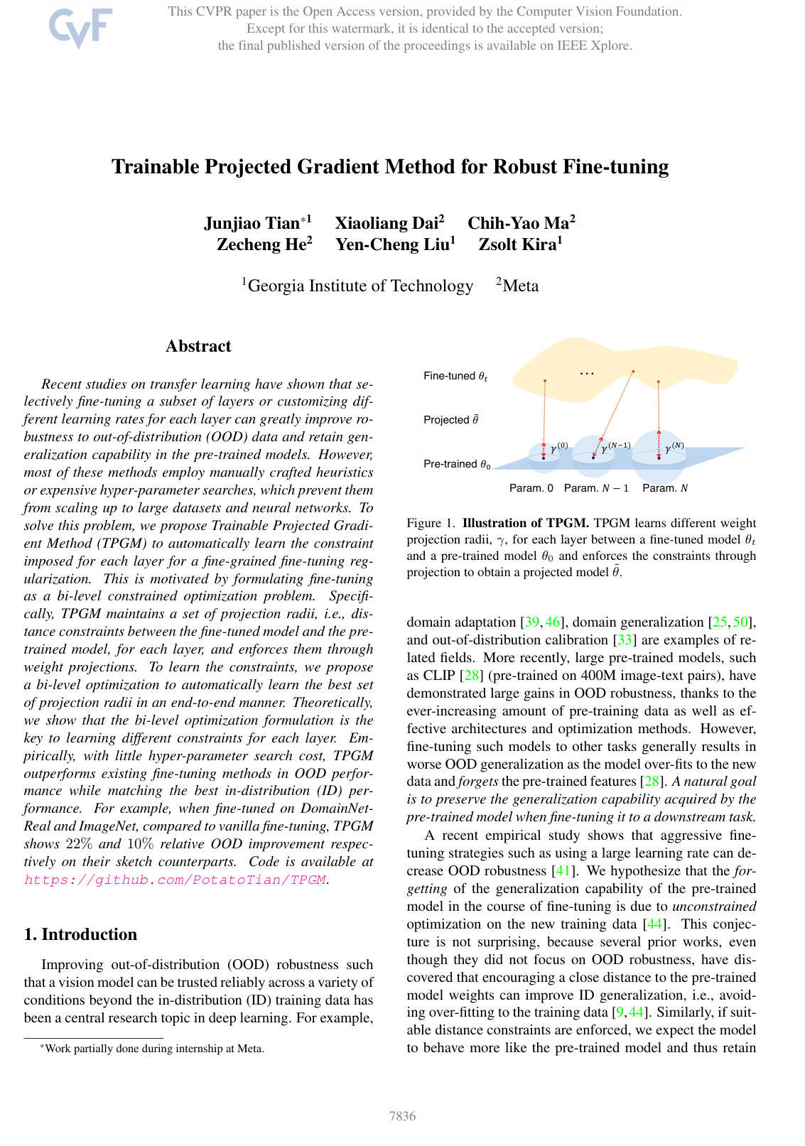
Recent studies on transfer learning have shown that selectively fine-tuning a subset of layers or customizing different learning rates for each layer can greatly improve robustness to out-of-distribution (OOD) data and retain generalization capability in the pre-trained models. However, most of these methods employ manually crafted heuristics or expensive hyper-parameter searches, which prevent them from scaling up to large datasets and neural networks. To solve this problem, we propose Trainable Projected Gradient Method (TPGM) to automatically learn the constraint imposed for each layer for a fine-grained fine-tuning regularization. This is motivated by formulating fine-tuning as a bi-level constrained optimization problem. Specifically, TPGM maintains a set of projection radii, i.e., distance constraints between the fine-tuned model and the pre-trained model, for each layer, and enforces them through weight projections. To learn the constraints, we propose a bi-level optimization to automatically learn the best set of projection radii in an end-to-end manner. Theoretically, we show that the bi-level optimization formulation is the key to learning different constraints for each layer. Empirically, with little hyper-parameter search cost, TPGM outperforms existing fine-tuning methods in OOD performance while matching the best in-distribution (ID) performance. For example, when fine-tuned on DomainNet-Real and ImageNet, compared to vanilla fine-tuning, TPGM shows 22% and 10% relative OOD improvement respectively on their sketch counterparts. Code is available at https://github.com/PotatoTian/TPGM.

Table of Contents

  • 1. Introduction
  • 2. Related Works
  • 3. Method
  • 3.1. Fine-tuning as a Bi-level Constrained Problem
  • 3.2. Projected Gradient Method
  • 3.3. Trainable Projected Gradient Method (TPGM)
  • 3.4. Bi-level Optimization is the Key
  • 4. Experiments
  • 4.1. Fine-Tuning a Pre-trained ResNet
  • 4.2. Fine-tuning a Pre-Trained Transformer
  • 5. Conclusion
  • References

Knowls

  1. Knowl 1 — Bi-level Constrained Optimization Formulation for Fine-tuning

    model/method

    Fine-tuning a pre-trained neural network while preserving its out-of-distribution (OOD) generalization is formulated as a bi-level constrained minimization problem. Let Dtr\mathcal{D}_{tr} denote the training dataset, Dval\mathcal{D}_{val} denote the validation dataset, and L(x,y;θ)\mathcal{L}(x, y; \theta) be the task loss function evaluated on input xx and label yy using model parameters θ\theta. Let θ0\theta_0 be the fixed initial weights of the pre-trained model and θt\theta_t be the trainable model parameters.

    The fine-tuning objective solves for outer hyperparameters λ\lambda (e.g., learning rate) and layer-wise distance constraint thresholds (projection radii) γ\gamma on the validation split, subject to the model being updated on the training split within a matrix-norm-induced distance constraint from θ0\theta_0:

    min⁡λ,γ∣(x,y)∈DvalL(x,y;arg⁡min⁡θt∣(x,y)∈DtrL(x,y;θt,λ),λ)s.t.∥θt−θ0∥∗≤γ\min_{\lambda, \gamma \mid (x,y) \in \mathcal{D}_{val}} \mathcal{L}\left(x, y; \arg\min_{\theta_t \mid (x,y) \in \mathcal{D}_{tr}} \mathcal{L}(x, y; \theta_t, \lambda), \lambda\right) \quad \text{s.t.} \quad \|\theta_t - \theta_0\|_* \le \gamma

    where ∥⋅∥∗\|\cdot\|_* represents a matrix norm (such as the Frobenius/L2L_2 norm or the Maximum Absolute Row Sum norm) applied independently to parameter groups across different layers. In this formulation, the inner optimization updates model parameters on Dtr\mathcal{D}_{tr}, whereas the outer optimization learns the constraint thresholds γ\gamma on Dval\mathcal{D}_{val} without calculating model parameter gradients on validation data.

  2. Knowl 2 — Trainable Projected Gradient Method (TPGM) Algorithm

    algorithm

    The Trainable Projected Gradient Method (TPGM) alternately performs unconstrained gradient updates on model parameters θ\theta using training data Dtr\mathcal{D}_{tr}, and updates layer-wise trainable projection radii γ\gamma using validation data Dval\mathcal{D}_{val}. Crucially, when updating γ\gamma, the model parameters θ\theta remain frozen to avoid validation data leakage.

    Input: Training set Dtr\mathcal{D}_{tr}, validation set Dval\mathcal{D}_{val}, pre-trained weights θ0\theta_0
    Input: Initial projection radii γ0=ϵ\gamma_0 = \epsilon, total steps TT, projection frequency fprojf_{proj}, inner projection steps TprojT_{proj}, learning rates ηtr,ζ\eta_{tr}, \zeta
    Output: Final projected model weights θ~T\tilde{\theta}_T
    Initialize θ~0=θ0\tilde{\theta}_0 = \theta_0, θ0\theta_0, and γ0=ϵ\gamma_0 = \epsilon
    for t=0t = 0 to T−1T - 1 do
        Sample (xtr,ytr)∼Dtr(x_{tr}, y_{tr}) \sim \mathcal{D}_{tr}
        θt+1=θt−ηtr∇θL(xtr,ytr;θ~t)\theta_{t+1} = \theta_t - \eta_{tr} \nabla_{\theta} \mathcal{L}(x_{tr}, y_{tr}; \tilde{\theta}_t)
        if t mod fproj==0t \bmod f_{proj} == 0 then
            γ(0)=γt\gamma^{(0)} = \gamma_t
            for τ=0\tau = 0 to Tproj−1T_{proj} - 1 do
                Sample (xval,yval)∼Dval(x_{val}, y_{val}) \sim \mathcal{D}_{val}
                θ~(τ)=Π(θ0,θt+1,γ(τ))\tilde{\theta}^{(\tau)} = \Pi(\theta_0, \theta_{t+1}, \gamma^{(\tau)})
                γ(τ+1)=γ(τ)−ζ∇γL(xval,yval;θ~(τ))\gamma^{(\tau+1)} = \gamma^{(\tau)} - \zeta \nabla_\gamma \mathcal{L}(x_{val}, y_{val}; \tilde{\theta}^{(\tau)})
            end for
            γt+1=γ(Tproj)\gamma_{t+1} = \gamma^{(T_{proj})}
            θ~t+1=Π(θ0,θt+1,γt+1)\tilde{\theta}_{t+1} = \Pi(\theta_0, \theta_{t+1}, \gamma_{t+1})
        else
            γt+1=γt\gamma_{t+1} = \gamma_t
            θ~t+1=θ~t\tilde{\theta}_{t+1} = \tilde{\theta}_t
        end if
    end for
    return θ~T\tilde{\theta}_T

    For convolutional backbones (e.g., ResNet), projection updates can be applied at every step (fproj=1,Tproj=1f_{proj} = 1, T_{proj} = 1). For vision transformer architectures exhibiting linear mode connectivity, projection can be executed once at the end of training (fproj=T−1,Tproj=200f_{proj} = T - 1, T_{proj} = 200).

  3. Knowl 3 — Closed-Form Projection Operators for Weight Constraints

    equation

    To enforce the layer-wise distance constraint ∥θt−θ0∥∗≤γ\|\theta_t - \theta_0\|_* \le \gamma efficiently during forward passes without nested numerical optimization, closed-form projection operators Π(θ0,θt,γ)\Pi(\theta_0, \theta_t, \gamma) are used.

    For the L2L_2 norm, the exact closed-form projection of model weights θt\theta_t onto an L2L_2-ball of radius γ>0\gamma > 0 centered at pre-trained weights θ0\theta_0 is:

    Πl2(θ0,θt,γ)=θ0+1max⁡(1,∥θt−θ0∥2γ)(θt−θ0)\Pi_{l2}(\theta_0, \theta_t, \gamma) = \theta_0 + \frac{1}{\max\left(1, \frac{\|\theta_t - \theta_0\|_2}{\gamma}\right)}(\theta_t - \theta_0)

    For the Maximum Absolute Row Sum (MARS) matrix norm, defined for a matrix AA as ∥A∥∞=max⁡j∑i∣Aj,i∣\|A\|_\infty = \max_j \sum_i |A_{j,i}|, the approximate closed-form projection operator is:

    Πmars(θ0,θt,γ)=θ0+1max⁡(1,∥θt−θ0∥∞γ)(θt−θ0)\Pi_{mars}(\theta_0, \theta_t, \gamma) = \theta_0 + \frac{1}{\max\left(1, \frac{\|\theta_t - \theta_0\|_\infty}{\gamma}\right)}(\theta_t - \theta_0)

    These operators allow gradients with respect to γ\gamma to propagate backward via standard automatic differentiation.

  4. Knowl 4 — Expected Loss Bound for Projected Linear Models

    theoretical result

    Consider an over-parameterized linear regression setup where target labels y∈Ry \in \mathbb{R} are generated by a ground-truth model θ∗∈Rd\theta^* \in \mathbb{R}^d such that y=θ∗Txy = {\theta^*}^T x for in-distribution data x∈Rdx \in \mathbb{R}^d. Let Xtr∈Rd×nX_{tr} \in \mathbb{R}^{d \times n} (n<dn < d) be the training matrix containing nn linearly independent training samples with labels Ytr=XtrTθ∗∈RnY_{tr} = X_{tr}^T \theta^* \in \mathbb{R}^n, and empirical loss L(Xtr,Ytr;θ)=∥XtrTθ−Ytr∥22\mathcal{L}(X_{tr}, Y_{tr}; \theta) = \|X_{tr}^T \theta - Y_{tr}\|_2^2.

    Let Xtr=UΣVTX_{tr} = U \Sigma V^T be the singular value decomposition where U∈Rd×nU \in \mathbb{R}^{d \times n} forms the basis for the span of training samples, and U⊥∈Rd×(d−n)U_\perp \in \mathbb{R}^{d \times (d-n)} forms the basis for the complementary orthogonal subspace. Any vector x∈Rdx \in \mathbb{R}^d decomposes as x=Uτ+U⊥τ⊥x = U\tau + U_\perp \tau_\perp with τ∈Rn\tau \in \mathbb{R}^n and τ⊥∈Rd−n\tau_\perp \in \mathbb{R}^{d-n}. Let τˉ=E[∥τ∥2]\bar{\tau} = \mathbb{E}[\|\tau\|_2] and τˉ⊥=E[∥τ⊥∥2]\bar{\tau}_\perp = \mathbb{E}[\|\tau_\perp\|_2].

    Let θ\theta be any minimizer of the empirical loss, θ0\theta_0 be the pre-trained model, ϵ=∥θ0−θ∗∥2\epsilon = \|\theta_0 - \theta^*\|_2 be the pre-trained initialization error, and θ~=θ0+α(θ−θ0)\tilde{\theta} = \theta_0 + \alpha(\theta - \theta_0) be the projected model with projection ratio α∈[0,1]\alpha \in [0, 1]. The expected loss over the full data distribution is upper bounded by:

    E[∣θ~Tx−y∣2]≤(1−α)ϵτˉ⏟in-span risk+(ϵ+α∥θ−θ0∥2)τˉ⊥⏟out-span risk\mathbb{E}\left[\left|\tilde{\theta}^T x - y\right|^2\right] \le \underbrace{(1 - \alpha)\epsilon \bar{\tau}}_{\text{in-span risk}} + \underbrace{\left(\epsilon + \alpha \|\theta - \theta_0\|_2\right)\bar{\tau}_\perp}_{\text{out-span risk}}

    This bound demonstrates that when the pre-trained model is already close to the ground truth (small ϵ\epsilon), α\alpha must be small (stronger projection toward θ0\theta_0) to minimize the out-span risk on unseen components. When ϵ\epsilon is large, α\alpha must be larger (weaker projection) to minimize the in-span error.

  5. Knowl 5 — Layer-Wise Regularization Depth Dependency

    empirical result

    When optimizing layer-wise projection radii γ\gamma using TPGM, the learned distance constraints exhibit a consistent structural pattern across network depth:

    1. Input and Lower Layers: TPGM learns significantly smaller projection radii γ\gamma for layers closer to the input (e.g., initial convolutional blocks in ResNet50 or early transformer blocks in ViT-B). This imposes strong regularization, preventing features from diverging from the pre-trained initialization.
    2. Output and Higher Layers: Layers closer to the classifier head (e.g., the final pooling layer in ResNet50 or the final transformer blocks in ViT-B) are assigned much larger projection radii γ\gamma, allowing greater capacity to adapt to the downstream task.

    This aligns with the principle that early neural network layers extract generalizable, transferable features where pre-trained weights are already near-optimal (low initial error ϵ\epsilon), whereas higher layers require task-specific adaptation.

  6. Knowl 6 — Controlled TPGM (TPGM-C) via Projection Radii Regularization

    model/method

    To analyze and control the trade-off between in-distribution (ID) accuracy and out-of-distribution (OOD) robustness, an L2L_2 regularization penalty on the trainable projection parameters γ\gamma is incorporated during the projection update step on Dval\mathcal{D}_{val}:

    Lproj(γ)=L(xval,yval;θ~)+μ∥γ∥22\mathcal{L}_{proj}(\gamma) = \mathcal{L}(x_{val}, y_{val}; \tilde{\theta}) + \mu \|\gamma\|_2^2

    where μ≥0\mu \ge 0 is a regularization hyperparameter governing constraint tightness. Larger values of μ\mu penalize large radii, forcing γ\gamma to remain smaller and projecting the fine-tuned model θt\theta_t closer to θ0\theta_0. Sweeping μ\mu from 0.00.0 to 4×10⁻³⁴ \times 10^{-3} traces out a Pareto frontier between ID performance and OOD generalization.

  7. Knowl 7 — DomainNet Out-of-Distribution Robustness with ResNet-50

    data/table

    Fine-tuning experiments on DomainNet (0.6M images, 345 classes) use the Real domain as the in-distribution (ID) training data and evaluate out-of-distribution (OOD) generalization across Sketch, Painting, Infograph, and Clipart domains. TPGM with MARS projection is compared against Vanilla Fine-Tuning (Vanilla FT), Linear Probing (LP), Partial Transfusion (PF), L2L_2-SP, MARS-SP, and LP-FT across CLIP pre-trained ResNet-50 and MOCO-V3 self-supervised ResNet-50 (100% Real data, 50 epochs, Adam optimizer, batch size 256, cosine LR schedule).

    Method ID (Real) Sketch Painting Infograph Clipart OOD Avg. ID Δ\Delta (%) OOD Δ\Delta (%)
    CLIP Pre-trained ResNet-50 (100% Data)
    Vanilla FT 80.93 (0.08) 31.81 (0.06) 41.02 (0.10) 20.29 (0.08) 43.59 (0.15) 34.18 0.00 0.00
    LP 52.56 (0.09) 20.05 (0.21) 24.92 (2.49) 19.18 (0.46) 21.15 (0.18) 21.33 -35.05 -37.60
    PF 78.27 (0.11) 36.77 (0.32) 42.13 (0.35) 24.71 (0.18) 43.31 (0.53) 36.73 -3.29 +7.46
    L2-SP 82.07 (0.09) 36.67 (0.11) 45.62 (0.35) 22.97 (0.42) 47.78 (0.30) 38.26 +1.40 +11.94
    MARS-SP 77.19 (0.63) 25.33 (1.07) 33.43 (2.06) 14.81 (0.43) 39.20 (0.74) 28.19 -4.62 -17.53
    LP-FT 80.82 (0.95) 34.85 (1.93) 44.03 (0.05) 22.23 (2.01) 46.13 (2.34) 36.81 -0.14 +7.69
    TPGM 83.64 (0.01) 38.78 (0.42) 43.11 (0.25) 28.70 (0.31) 48.01 (0.25) 39.65 +3.34 +16.01
    MOCO-V3 Pre-trained ResNet-50 (100% Data)
    Vanilla FT 81.99 (0.03) 31.52 (0.33) 42.89 (0.53) 18.51 (0.28) 44.98 (0.24) 34.47 0.00 0.00
    LP 73.01 (0.03) 24.10 (0.23) 39.56 (0.15) 12.27 (0.02) 30.38 (0.08) 26.58 -10.96 -22.90
    PF 78.27 (0.03) 27.72 (0.07) 39.74 (0.12) 15.56 (0.08) 38.18 (0.12) 30.30 -4.55 -12.11
    L2-SP 81.51 (0.02) 34.91 (0.22) 45.76 (0.16) 18.97 (0.11) 45.29 (0.18) 36.23 -0.59 +5.09
    MARS-SP 81.89 (0.01) 34.44 (2.54) 45.05 (1.91) 19.97 (1.48) 46.36 (1.29) 36.45 -0.13 +5.74
    LP-FT 82.92 (0.01) 34.50 (0.22) 45.42 (0.31) 20.12 (0.43) 47.11 (0.27) 36.79 +1.13 +6.72
    TPGM 82.66 (0.13) 35.35 (0.33) 46.20 (0.20) 20.13 (0.12) 45.75 (0.12) 36.86 +0.82 +6.91

    TPGM achieves the highest average OOD accuracy across both pre-training paradigms (39.65% on CLIP and 36.86% on MOCO-V3) while simultaneously achieving superior or matched ID accuracy compared to vanilla fine-tuning.

  8. Knowl 8 — Fine-Tuning Robustness under Subsampled Training Data

    data/table

    When in-distribution training data on DomainNet-Real is subsampled to 10% of its original size (trained for 150 epochs), standard fine-tuning methods suffer severe overfitting and degradation in both ID and OOD accuracy. TPGM automatically tightens projection radii γ\gamma across all layers via validation feedback, mitigating overfitting.

    Method ID (Real) Sketch Painting Infograph Clipart OOD Avg. ID Δ\Delta (%) OOD Δ\Delta (%)
    Vanilla FT 57.35 (1.43) 17.48 (0.68) 25.60 (0.70) 10.30 (1.57) 23.01 (0.65) 19.10 0.00 0.00
    LP 47.19 (0.93) 17.81 (0.25) 22.71 (2.08) 17.13 (0.75) 17.59 (0.69) 18.81 -17.71 -1.52
    PF 71.04 (0.91) 27.87 (1.04) 38.31 (1.05) 19.85 (0.70) 33.92 (1.53) 29.99 +23.86 +57.01
    L2-SP 61.41 (0.92) 22.61 (0.52) 30.48 (0.42) 12.28 (0.50) 26.59 (0.57) 22.99 +7.08 +20.37
    MARS-SP 52.53 (0.84) 15.34 (0.54) 21.57 (0.45) 8.49 (0.60) 19.96 (0.01) 16.34 -8.41 -14.44
    LP-FT 64.11 (0.78) 20.54 (0.27) 30.89 (0.41) 13.58 (0.63) 29.55 (0.82) 23.64 +11.78 +23.77
    TPGM 73.16 (1.27) 29.88 (0.81) 36.80 (1.42) 19.72 (0.12) 35.28 (0.74) 30.42 +27.56 +59.27

    Compared to vanilla fine-tuning, TPGM improves ID accuracy by +27.56% (from 57.35% to 73.16%) and average OOD accuracy by +59.27% (from 19.10% to 30.42%), demonstrating automatic adaptation to small dataset regimes.

  9. Knowl 9 — ImageNet and OOD Benchmark Performance on Vision Transformers

    data/table

    Using a CLIP pre-trained ViT-B model initialized with zero-shot text classifier weights, fine-tuning is evaluated on ImageNet-1K and tested for OOD robustness on ImageNet-V2 (ID distribution shift), ImageNet-A, ImageNet-R, and ImageNet-S without subsampling classes. TPGM (L2L_2 projection, fproj=T−1,Tproj=200f_{proj} = T-1, T_{proj} = 200) is compared against full and parameter-efficient fine-tuning baselines, zero-shot CLIP, and WiSE-FT.

    Method ImageNet ImageNet-V2 ImageNet-A ImageNet-R ImageNet-S ID Avg. OOD Avg. ID Δ\Delta (%) OOD Δ\Delta (%)
    Vanilla FT 84.20 (0.02) 75.08 (0.11) 26.52 (0.12) 46.45 (0.06) 48.90 (0.58) 79.64 40.63 0.00 0.00
    LP 77.99 (0.02) 67.74 (0.04) 27.13 (0.06) 50.71 (0.07) 46.47 (0.04) 72.86 41.44 -8.51 +2.00
    BitFit 78.02 (0.12) 67.69 (0.15) 27.19 (0.28) 50.66 (0.31) 46.50 (0.29) 72.85 41.45 -8.42 +2.45
    L2-SP 84.10 (0.02) 75.05 (0.11) 26.19 (0.45) 46.58 (0.09) 48.51 (0.12) 79.58 40.43 -0.08 -0.49
    LP-FT 83.50 (0.15) 73.95 (0.12) 25.62 (0.23) 46.21 (0.22) 48.83 (0.19) 78.73 40.22 -1.15 -1.00
    Zero-Shot 67.68 (N/A) 61.41 (N/A) 30.60 (N/A) 56.77 (N/A) 45.53 (N/A) 64.54 44.30 -18.91 +8.64
    WiSE 82.11 (0.14) 73.61 (0.13) 36.11 (0.16) 61.77 (0.08) 54.16 (0.07) 77.86 50.68 -2.23 +24.75
    TPGM-C 82.41 (0.07) 73.91 (0.21) 36.79 (0.14) 62.48 (0.10) 54.91 (0.12) 78.16 51.39 -1.86 +26.51
    TPGM 84.19 (0.03) 75.41 (1.61) 34.29 (2.11) 57.19 (0.54) 54.38 (0.19) 79.80 48.62 +0.20 +19.69

    TPGM matches Vanilla FT in ID accuracy (79.80% vs 79.64% ID Avg.) while improving average OOD accuracy by +19.69% (48.62% vs 40.63%). Under controlled settings matching WiSE's ID accuracy, TPGM-C achieves 51.39% average OOD accuracy compared to 50.68% for WiSE.

Coverage note — Omitted specific appendix-only implementation details such as total variation smoothing hyperparameter sweeps, CLIP ViT-L exploratory curves, and linear probe zero-shot formulation derivations as they support or duplicate the core method, theory, and benchmarks presented in the main paper.

References

  1. 1.Qiang Chen, Philippe Montesinos, Quan Sen Sun, Peng Ann Heng, et al. Adaptive total variation denoising based on difference curvature. Image and vision computing, 28(3):298–306, 2010. 4, 12
  2. 2.Xinlei Chen, Saining Xie, and Kaiming He. An empirical study of training self-supervised vision transformers. In Proceedings of the IEEE/CVF International Conference on Computer Vision, pages 9640–9649, 2021. 5
  3. 3.Laurent Condat. A direct algorithm for 1-d total variation denoising. IEEE Signal Processing Letters, 20(11):1054–1057, 2013. 4, 12
  4. 4.Jia Deng, Wei Dong, Richard Socher, Li-Jia Li, Kai Li, and Li Fei-Fei. Imagenet: A large-scale hierarchical image database. In 2009 IEEE conference on computer vision and pattern recognition, pages 248–255. Ieee, 2009. 2, 5
  5. 5.Terrance DeVries and Graham W Taylor. Learning confidence for out-of-distribution detection in neural networks. arXiv preprint arXiv:1802.04865, 2018. 3
  6. 6.Simon S Du, Wei Hu, Sham M Kakade, Jason D Lee, and Qi Lei. Few-shot learning via learning the representation, provably. arXiv preprint arXiv:2002.09434, 2020. 4
  7. 7.Jonathan Frankle, Gintare Karolina Dziugaite, Daniel Roy, and Michael Carbin. Linear mode connectivity and the lottery ticket hypothesis. In International Conference on Machine Learning, pages 3259–3269. PMLR, 2020. 3
  8. 8.Jonathan Godwin, Michael Schaarschmidt, Alexander L Gaunt, Alvaro Sanchez-Gonzalez, Yulia Rubanova, Petar Veličković, James Kirkpatrick, and Peter Battaglia. Simple gnn regularisation for 3d molecular property prediction and beyond. In International conference on learning representations, 2021. 2
  9. 9.Henry Gouk, Timothy M Hospedales, and Massimiliano Pontil. Distance-based regularisation of deep networks for fine-tuning. ICLR, 2021. 1, 3, 6, 7, 12
  10. 10.Chuan Guo, Geoff Pleiss, Yu Sun, and Kilian Q Weinberger. On calibration of modern neural networks. In International conference on machine learning, pages 1321–1330. PMLR, 2017. 2
  11. 11.Yunhui Guo, Honghui Shi, Abhishek Kumar, Kristen Grauman, Tajana Rosing, and Rogerio Feris. Spottune: transfer learning through adaptive fine-tuning. In Proceedings of the IEEE/CVF conference on computer vision and pattern recognition, pages 4805–4814, 2019. 2
  12. 12.Kaiming He, Xinlei Chen, Saining Xie, Yanghao Li, Piotr Dollár, and Ross Girshick. Masked autoencoders are scalable vision learners. In Proceedings of the IEEE/CVF Conference on Computer Vision and Pattern Recognition, pages 16000–16009, 2022. 13
  13. 13.Kaiming He, Ross Girshick, and Piotr Dollár. Rethinking imagenet pre-training. In Proceedings of the IEEE/CVF International Conference on Computer Vision, pages 4918–4927, 2019. 2
  14. 14.Kaiming He, Xiangyu Zhang, Shaoqing Ren, and Jian Sun. Deep residual learning for image recognition. In Proceedings of the IEEE conference on computer vision and pattern recognition, pages 770–778, 2016. 5, 12
  15. 15.Dan Hendrycks, Steven Basart, Norman Mu, Saurav Kadavath, Frank Wang, Evan Dorundo, Rahul Desai, Tyler Zhu, Samyak Parajuli, Mike Guo, et al. The many faces of robustness: A critical analysis of out-of-distribution generalization. In Proceedings of the IEEE/CVF International Conference on Computer Vision, pages 8340–8349, 2021. 5
  16. 16.Dan Hendrycks, Kimin Lee, and Mantas Mazeika. Using pre-training can improve model robustness and uncertainty. In International Conference on Machine Learning, pages 2712–2721. PMLR, 2019. 3
  17. 17.Dan Hendrycks, Kevin Zhao, Steven Basart, Jacob Steinhardt, and Dawn Song. Natural adversarial examples. In Proceedings of the IEEE/CVF Conference on Computer Vision and Pattern Recognition, pages 15262–15271, 2021. 5
  18. 18.Alfredo N Iusem. On the convergence properties of the projected gradient method for convex optimization. Computational & Applied Mathematics, 22:37–52, 2003. 3
  19. 19.Fahdi Kanavati and Masayuki Tsuneki. Partial transfusion: on the expressive influence of trainable batch norm parameters for transfer learning. In Medical Imaging with Deep Learning, pages 338–353. PMLR, 2021. 6, 7, 12
  20. 20.Diederik P Kingma and Jimmy Ba. Adam: A method for stochastic optimization. arXiv preprint arXiv:1412.6980, 2014. 4, 5, 12
  21. 21.Ananya Kumar et al. Fine-tuning can distort pretrained features and underperform out-of-distribution. ICLR, 2022. 3, 6, 7, 8, 12, 13
  22. 22.Yoonho Lee, Annie S Chen, Fahim Tajwar, Ananya Kumar, Huaxiu Yao, Percy Liang, and Chelsea Finn. Surgical fine-tuning improves adaptation to distribution shifts. arXiv preprint arXiv:2210.11466, 2022. 2
  23. 23.Xingjian Li, Haoyi Xiong, Hanchao Wang, Yuxuan Rao, Liping Liu, Zeyu Chen, and Jun Huan. Delta: Deep learning transfer using feature map with attention for convolutional networks. arXiv preprint arXiv:1901.09229, 2019. 2
  24. 24.Ilya Loshchilov and Frank Hutter. Decoupled weight decay regularization. arXiv preprint arXiv:1711.05101, 2017. 13
  25. 25.Krikamol Muandet, David Balduzzi, and Bernhard Schölkopf. Domain generalization via invariant feature representation. In International Conference on Machine Learning, pages 10–18. PMLR, 2013. 1
  26. 26.Behnam Neyshabur, Hanie Sedghi, and Chiyuan Zhang. What is being transferred in transfer learning? Advances in neural information processing systems, 33:512–523, 2020. 2, 5
  27. 27.Xingchao Peng, Qinxun Bai, Xide Xia, Zijun Huang, Kate Saenko, and Bo Wang. Moment matching for multi-source domain adaptation. In Proceedings of the IEEE/CVF international conference on computer vision, pages 1406–1415, 2019. 2, 5
  28. 28.Alec Radford, Jong Wook Kim, Chris Hallacy, Aditya Ramesh, Gabriel Goh, Sandhini Agarwal, Girish Sastry, Amanda Askell, Pamela Mishkin, Jack Clark, et al. Learning transferable visual models from natural language supervision. In International Conference on Machine Learning, pages 8748–8763. PMLR, 2021. 1, 3, 5, 7, 8, 13, 14
  29. 29.Maithra Raghu, Chiyuan Zhang, Jon Kleinberg, and Samy Bengio. Transfusion: Understanding transfer learning for medical imaging. Advances in neural information processing systems, 32, 2019. 2, 5
  30. 30.Benjamin Recht, Rebecca Roelofs, Ludwig Schmidt, and Vaishaal Shankar. Do imagenet classifiers generalize to imagenet? In International Conference on Machine Learning, pages 5389–5400. PMLR, 2019. 5
  31. 31.Zhiqiang Shen, Zechun Liu, Jie Qin, Marios Savvides, and Kwang-Ting Cheng. Partial is better than all: Revisiting fine-tuning strategy for few-shot learning. In Proceedings of the AAAI Conference on Artificial Intelligence, volume 35, pages 9594–9602, 2021. 2
  32. 32.Christian Szegedy, Vincent Vanhoucke, Sergey Ioffe, Jon Shlens, and Zbigniew Wojna. Rethinking the inception architecture for computer vision. In Proceedings of the IEEE conference on computer vision and pattern recognition, pages 2818–2826, 2016. 13
  33. 33.Junjiao Tian, Dylan Yung, Yen-Chang Hsu, and Zsolt Kira. A geometric perspective towards neural calibration via sensitivity decomposition. Advances in Neural Information Processing Systems, 34:26358–26369, 2021. 1
  34. 34.Hugo Touvron, Matthieu Cord, Matthijs Douze, Francisco Massa, Alexandre Sablayrolles, and Hervé Jégou. Training data-efficient image transformers & distillation through attention. In International Conference on Machine Learning, pages 10347–10357. PMLR, 2021. 7, 12, 13
  35. 35.Hugo Touvron, Matthieu Cord, and Hervé Jégou. Deit iii: Revenge of the vit. arXiv preprint arXiv:2204.07118, 2022. 7, 12
  36. 36.Nilesh Tripuraneni, Michael Jordan, and Chi Jin. On the theory of transfer learning: The importance of task diversity. Advances in Neural Information Processing Systems, 33:7852–7862, 2020. 4
  37. 37.Ashish Vaswani, Noam Shazeer, Niki Parmar, Jakob Uszkoreit, Llion Jones, Aidan N Gomez, Łukasz Kaiser, and Illia Polosukhin. Attention is all you need. Advances in neural information processing systems, 30, 2017. 2, 5, 7, 12
  38. 38.Haohan Wang, Songwei Ge, Zachary Lipton, and Eric P Xing. Learning robust global representations by penalizing local predictive power. Advances in Neural Information Processing Systems, 32, 2019. 5
  39. 39.Mei Wang and Weihong Deng. Deep visual domain adaptation: A survey. Neurocomputing, 312:135–153, 2018. 1
  40. 40.Yang Wen, Leiting Chen, Yu Deng, and Chuan Zhou. Rethinking pre-training on medical imaging. Journal of Visual Communication and Image Representation, 78:103145, 2021. 2
  41. 41.Mitchell Wortsman, Gabriel Ilharco, Jong Wook Kim, Mike Li, Simon Kornblith, Rebecca Roelofs, Raphael Gontijo Lopes, Hannaneh Hajishirzi, Ali Farhadi, Hongseok Namkoong, et al. Robust fine-tuning of zero-shot models. In Proceedings of the IEEE/CVF Conference on Computer Vision and Pattern Recognition, pages 7959–7971, 2022. 1, 2, 3, 4, 5, 7, 8, 13, 14
  42. 42.Sen Wu, Hongyang R Zhang, and Christopher Ré. Understanding and improving information transfer in multi-task learning. arXiv preprint arXiv:2005.00944, 2020. 4
  43. 43.Sang Michael Xie, Ananya Kumar, Robbie Jones, Fereshte Khani, Tengyu Ma, and Percy Liang. In-n-out: Pre-training and self-training using auxiliary information for out-of-distribution robustness. arXiv preprint arXiv:2012.04550, 2020. 4
  44. 44.LI Xuhong, Yves Grandvalet, and Franck Davoine. Explicit inductive bias for transfer learning with convolutional networks. In International Conference on Machine Learning, pages 2825–2834. PMLR, 2018. 1, 2, 3, 6, 7, 8, 12, 13
  45. 45.Jason Yosinski, Jeff Clune, Yoshua Bengio, and Hod Lipson. How transferable are features in deep neural networks? Advances in neural information processing systems, 27, 2014. 2, 5
  46. 46.Kaichao You, Mingsheng Long, Zhangjie Cao, Jianmin Wang, and Michael I Jordan. Universal domain adaptation. In Proceedings of the IEEE/CVF conference on computer vision and pattern recognition, pages 2720–2729, 2019. 1
  47. 47.Sangdoo Yun, Dongyoon Han, Seong Joon Oh, Sanghyuk Chun, Junsuk Choe, and Youngjoon Yoo. Cutmix: Regularization strategy to train strong classifiers with localizable features. In Proceedings of the IEEE/CVF international conference on computer vision, pages 6023–6032, 2019. 13
  48. 48.Elad Ben Zaken, Shauli Ravfogel, and Yoav Goldberg. Bitfit: Simple parameter-efficient fine-tuning for transformer-based masked language-models. arXiv preprint arXiv:2106.10199, 2021. 8, 13
  49. 49.Hongyi Zhang, Moustapha Cisse, Yann N Dauphin, and David Lopez-Paz. mixup: Beyond empirical risk minimization. arXiv preprint arXiv:1710.09412, 2017. 13
  50. 50.Kaiyang Zhou, Ziwei Liu, Yu Qiao, Tao Xiang, and Chen Change Loy. Domain generalization: A survey. IEEE Transactions on Pattern Analysis and Machine Intelligence, 2022. 1

Citation

MLA
Tian, J., et al. “Trainable Projected Gradient Method for Robust Fine-tuning”. Conference on Computer Vision and Pattern Recognition 2023, 2023, http://arxiv.org/abs/2303.10720v2.
APA
Tian, J., Dai, X., Ma, C.-Y., He, Z., Liu, Y.-C., & Kira, Z. (2023). Trainable Projected Gradient Method for Robust Fine-tuning. Conference on Computer Vision and Pattern Recognition 2023. http://arxiv.org/abs/2303.10720v2
Chicago
Tian, J., X. Dai, C.-Y. Ma, Z. He, Y.-C. Liu, and Z. Kira. 2023. “Trainable Projected Gradient Method for Robust Fine-tuning”. Conference on Computer Vision and Pattern Recognition 2023. http://arxiv.org/abs/2303.10720v2.
Harvard
Tian, J. et al. (2023) “Trainable Projected Gradient Method for Robust Fine-tuning”, Conference on Computer Vision and Pattern Recognition 2023 [Preprint]. Available at: http://arxiv.org/abs/2303.10720v2.
Vancouver
1. Tian J, Dai X, Ma C-Y, He Z, Liu Y-C, Kira Z (2023) Trainable Projected Gradient Method for Robust Fine-tuning. Conference on Computer Vision and Pattern Recognition 2023

BibTeX

@article{tian2023trainable,
  title = {Trainable Projected Gradient Method for Robust Fine-tuning},
  author = {Tian, Junjiao and Dai, Xiaoliang and Ma, Chih-Yao and He, Zecheng and Liu, Yen-Cheng and Kira, Zsolt},
  year = {2023},
  journal = {Conference on Computer Vision and Pattern Recognition 2023},
  url = {http://arxiv.org/abs/2303.10720v2},
  eprint = {2303.10720}
}
Metadata:arXiv

Source Code

This paper has an official code repository available. Click below to access the source code.

View Repository

Access the Paper

This paper is available from its original source. Click below to access the PDF.

Open PDF
License: IEEE