Tri-Perspective view Decomposition for Geometry-Aware Depth Completion

Zhiqiang YanYuankai LinKun WangYupeng ZhengYufei WangZhenyu ZhangJun LiJian Yang

article2024CVPR71 citations

Proposes a tri-perspective view decomposition framework that models structural 3D geometry across top, front, and side projections using spherical convolutions and geometric spatial propagation to achieve superior depth completion on standard benchmarks and real-world smartphone data.

Listen

Accurate 3D depth perception is critical for autonomous driving, robotics, and mobile augmented reality. However, real-world depth sensors such as LiDAR and time-of-flight (TOF) cameras produce highly sparse measurements, with outdoor point cloud densities often dropping below 5%. Existing depth completion methods either process data entirely within 2D image space—losing critical 3D spatial geometry—or attempt to process raw 3D point clouds directly, which introduces significant computational complexity and struggles with uneven point distributions over long distances.

The article demonstrates a new framework called Tri-Perspective View Decomposition (TPVD) to reconstruct high-resolution, dense depth maps while explicitly preserving 3D geometric structure. The main objective was to develop an accurate, computationally efficient architecture that overcomes the sparsity and distance-varying characteristics of raw 3D sensor data.

The authors designed a framework that converts raw 3D point clouds into three orthogonal 2D projections (top, side, and front views) and refines them using standard 2D convolutions. To preserve structural accuracy, TPVD introduces a recurrent 2D-3D-2D fusion process that projects intermediate 2D features into 3D spherical space, applies distance-aware convolutions to normalize point density across varying ranges, and projects the updated representations back to 2D. A geometric refinement network then enforces spatial consistency across all three views. The researchers evaluated the method across standard benchmarks, including the outdoor KITTI dataset and indoor NYUv2 and SUN RGBD datasets, while also introducing a new real-world mobile depth dataset (TOFDC) comprising 10,000 paired RGB-D images collected via smartphone TOF sensors.

The experimental findings show that TPVD establishes state-of-the-art performance across all benchmark tests. First, on the competitive outdoor KITTI benchmark, TPVD achieved first place across all standard evaluation metrics, outperforming the five most recent leading models by an average margin of 15.98 mm in root mean squared error. Second, on the newly created TOFDC mobile dataset, the approach reduced root mean squared error by 15.6% and relative error by 33.3% compared to the strongest 3D-assisted baseline. Third, computational efficiency evaluations demonstrated that TPVD requires 134 billion fewer floating-point operations than comparable high-performing models, resulting in faster training and a test runtime of 8.82 frames per second. Finally, the framework maintained robustness across diverse stress conditions, including depth-only inputs without camera imagery, varying levels of point cloud sparsity, and synthetic adverse weather conditions such as fog, rain, and low lighting.

These findings indicate that 3D geometric awareness can be achieved without relying on resource-intensive raw point-cloud or voxel networks. By processing spatial information across decomposed 2D views and recurrent spherical transforms, systems can achieve higher geometric fidelity at lower computational cost. For deployment teams in autonomous vehicles and edge computing devices, this translates directly to safer navigation, reduced processing latency, and lower onboard hardware overhead.

Decision-makers and engineering teams developing vision-based perception systems should consider adopting multi-view 2D decomposition techniques as an alternative to native 3D processing pipelines. Prior to full-scale production deployment, organizations should conduct on-vehicle pilot testing to validate real-time frame rates under specific hardware constraints and evaluate sensor integration across varied weather conditions.

The primary limitation of the study is that adverse weather and lighting conditions were evaluated predominantly on synthetic virtual benchmarks rather than exhaustive physical-world edge cases. Nonetheless, given the consistent outperformance across multiple established public benchmarks and the newly introduced mobile dataset, confidence in the reported accuracy and structural stability remains high.

geometry-aware depth completion tri-perspective view decomposition distance-aware spherical convolution

arXiv: 2403.15008

Paper: Dynamic Spatial Propagation Network for Depth Completion, Yuankai Lin et al. (2022). It introduces dynamic affinity learning for spatial propagation networks in depth completion, which directly establishes the foundation for the Geometric Spatial Propagation Network (GSPN) developed in this work.
Paper: SUN RGB-D: A RGB-D scene understanding benchmark suite, Shuran Song et al. (2015). It establishes the standard SUN RGB-D benchmark dataset and evaluation protocol for RGB-D indoor scene geometry completion and understanding utilized by the source.
Paper: BEVFormer: Learning Bird's-Eye-View Representation from Multi-Camera Images via Spatiotemporal Transformers, Zhiqi Li et al. (2022). It introduces foundational multi-view and bird's-eye-view projection and spatial aggregation architectures for autonomous driving that inform multi-perspective view representations.
Paper: Depth Map Prediction from a Single Image using a Multi-Scale Deep Network, David Eigen et al. (2014). It presents foundational multi-scale deep network architectures and training protocols for depth prediction on KITTI and NYU Depth benchmarks.

Paper: Depth Anything V2, Lihe Yang et al. (2024). It extends metric geometric surface estimation by presenting a foundation model trained on synthetic data and scaled pseudo-labels for high-resolution dense depth recovery across complex scenes.
Paper: Depth Pro: Sharp Monocular Metric Depth in Less Than a Second, Alexey Bochkovskiy et al. (2025). It builds on zero-shot metric depth estimation to recover sharp geometric boundaries and high-resolution depth maps without relying on sparse sensor measurements.
Paper: VGGT: Visual Geometry Grounded Transformer, Jianyuan Wang et al. (2025). It generalizes multi-view and single-view visual geometry prediction into an end-to-end feed-forward transformer framework that jointly estimates depth, poses, and dense 3D point structures.
Paper: Symphonize 3D Semantic Scene Completion with Contextual Instance Queries, Haoyi Jiang et al. (2024). It advances 3D scene completion by integrating instance-level queries with depth rectification to resolve fine-grained geometric occupancy and semantic categories.

Cover for Tri-Perspective view Decomposition for Geometry-Aware Depth Completion

Abstract

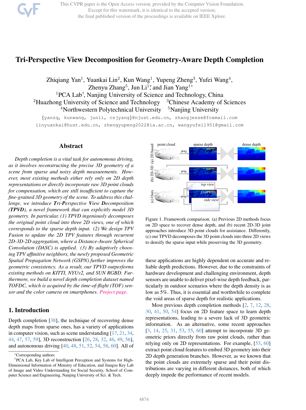
Depth completion is a vital task for autonomous driving, as it involves reconstructing the precise 3D geometry of a scene from sparse and noisy depth measurements. However, most existing methods either rely only on 2D depth representations or directly incorporate raw 3D point clouds for compensation, which are still insufficient to capture the fine-grained 3D geometry of the scene. To address this challenge, we introduce Tri-Perspective View Decomposition (TPVD), a novel framework that can explicitly model 3D geometry. In particular, (1) TPVD ingeniously decomposes the original point cloud into three 2D views, one of which corresponds to the sparse depth input. (2) We design TPV Fusion to update the 2D TPV features through recurrent 2D-3D-2D aggregation, where a Distance-Aware Spherical Convolution (DASC) is applied. (3) By adaptively choosing TPV affinitive neighbors, the newly proposed Geometric Spatial Propagation Network (GSPN) further improves the geometric consistency. As a result, our TPVD outperforms existing methods on KITTI, NYUv2, and SUN RGBD. Furthermore, we build a novel depth completion dataset named TOFDC, which is acquired by the time-of-flight (TOF) sensor and the color camera on smartphones. Project page.

Keywords

geometry-aware depth completion tri-perspective view decomposition distance-aware spherical convolution geometric spatial propagation TPV fusion panoramic depth completion point cloud decomposition

1. Introduction
2. Related Work
3. TPVD
3.1. Overview
3.2. TPV Projection
3.3. TPV Interaction
3.4. Geometry-Aware Refinement
4. TOFDC
5. Experiments
5.1. Datasets
5.2. Comparison with State-of-the-arts
5.3. Generalization Capability
5.4. Ablation Studies
6. Conclusion
Acknowledgements
References

Knowls

Knowl 1 — Tri-perspective view decomposition framework
model/method
TPVD is a depth-completion framework that uses both sparse depth and, in its standard configuration, an aligned RGB image to recover dense depth while preserving 3D geometry. It first converts the sparse depth measurements into a 3D point representation, projects that representation into orthogonal top, front, and side 2D views, and processes the views with separate 2D subnetworks. The sparse input itself is retained in the front view. TPVD then alternates 2D and 3D processing through recurrent TPV Fusion, which densifies the projected views, aggregates their features in 3D, refines the geometry in spherical coordinates, and projects the result back into the three 2D views. Finally, Geometric Spatial Propagation Network (GSPN) propagates information across the three views and their joint 3D projection to refine the coarse depth prediction. The standard TPV Fusion uses four recurrent steps; the final GSPN configuration uses nine neighbors and four propagation iterations.
Knowl 2 — Sparse-depth projection into three orthogonal views
equation
Let $\mathbf{S}\in\mathbb{R}^{H\times W}$ be a sparse depth map, let $\mathbf{m}\in\{0,1\}^{H\times W}$ be its validity mask with $m_{uv}=1$ at measured pixels, and let $\mathbf{P}$ be the 3D point representation generated from the valid measurements. The TPV projection operator $\mathcal{P}_{\mathrm{tpv}}$ maps $\mathbf{P}$ into a top-view map $\mathbf{V}_t\in\mathbb{R}^{W\times D}$ , a side-view map $\mathbf{V}_s\in\mathbb{R}^{D\times H}$ , and a front-view map $\mathbf{V}_f\in\mathbb{R}^{H\times W}$ , where $D$ is the number of discretized cells along the depth-related axis:
$\mathbf{V}_t,\mathbf{V}_s,\mathbf{V}_f=\mathcal{P}_{\mathrm{tpv}}(\mathbf{P}),\qquad \mathbf{V}_f^{\mathrm{new}}=\mathbf{S}+(1-\mathbf{m})\odot\mathbf{V}_f.$
Here $\odot$ denotes elementwise multiplication. The update preserves every observed depth value in the front view and uses the projected point representation only at pixels where the sparse input is invalid. Consequently, the three views jointly retain the original 3D point arrangement while making the sparse measurements amenable to ordinary 2D convolutions.
Knowl 3 — Recurrent 2D–3D–2D TPV Fusion
model/method
At decoder layer $i\in\{1,2,3,4\}$ , three subnetworks encode the top, side, and front views; the front subnetwork can additionally use the aligned RGB image. Their intermediate features are $\mathbf{F}_t^i\in\mathbb{R}^{W_i\times D_i\times C_i}$ , $\mathbf{F}_s^i\in\mathbb{R}^{D_i\times H_i\times C_i}$ , and $\mathbf{F}_f^i\in\mathbb{R}^{H_i\times W_i\times C_i}$ , where $H_i,W_i,D_i$ are the layer resolutions and $C_i$ is the channel count.

A TPV Fusion iteration has three stages. First, the three 2D features are jointly back-projected into Cartesian 3D coordinates by $\mathcal{P}_{\mathrm{tpv}}^{-1}$ ; k-nearest-neighbor aggregation followed by an MLP, denoted $h_{\mathrm{km}}$ , produces a refined Cartesian feature. Second, this feature is transformed to spherical coordinates and processed by the distance-aware spherical convolution described separately. Third, the refined spherical feature is inverse-transformed and projected back into the three TPV planes, after which 2D convolutions update the three view features:
$\mathbf{F}_{xyz}^{i}=\mathcal{P}_{\mathrm{tpv}}^{-1}(\mathbf{F}_t^i,\mathbf{F}_s^i,\mathbf{F}_f^i),\qquad \widetilde{\mathbf{F}}_{xyz}^{i}=h_{\mathrm{km}}(\mathbf{F}_{xyz}^{i}),$ $\widetilde{\mathbf{F}}_t^i,\widetilde{\mathbf{F}}_s^i,\widetilde{\mathbf{F}}_f^i =h_{2c}\!\left(\mathcal{P}_{\mathrm{tpv}}\left(\mathcal{P}_{\mathrm{sph}}^{-1}(\widetilde{\mathbf{F}}_{r\theta\varphi}^{i})\right)\right),$
where $\mathcal{P}_{\mathrm{sph}}$ and $\mathcal{P}_{\mathrm{sph}}^{-1}$ convert between Cartesian and spherical coordinates, and $h_{2c}$ is a 2D convolutional update. The 2D stages produce more valid projected pixels for later 3D aggregation, while the 3D stages return geometric information to the 2D stages; this complementary interaction is the central mechanism used to densify the input without discarding its spatial structure.
Knowl 4 — Distance-aware spherical convolution
equation
TPVD applies DASC to a spherical feature $\mathbf{F}_{r\theta\varphi}^{i}$ indexed by radius $r$ , polar angle $\theta$ , and azimuth $\varphi$ . The spherical domain is partitioned by a slicing operator $\mathcal{S}$ into subareas $\{A_{\mathrm{sph}}^1,\ldots,A_{\mathrm{sph}}^J\}$ . The subarea volume increases with distance $d$ , satisfying $|A_{\mathrm{sph}}^j|\propto d$ , so distant and nearby points are represented with different spatial cell sizes. A flattening operator $\mathcal{F}$ converts the spherical subareas into cubic blocks, a conventional 3D convolution $h_{3c}$ processes those blocks with a $3\times3\times3$ kernel and stride $1$ , and $\mathcal{F}^{-1}$ restores the spherical arrangement:
$\widetilde{\mathbf{F}}_{r\theta\varphi}^{i} =\mathcal{F}^{-1}\!\left(h_{3c}\left(\mathcal{F}\left(\mathcal{S}\left(\mathbf{F}_{r\theta\varphi}^{i}\right)\right)\right)\right).$
The construction is intended to compensate for the distance-dependent density of LiDAR points. In the paper's non-empty-cell analysis, cubic versus spherical representations have respectively $15.4\%$ versus $17.6\%$ non-empty cells at $0$ – $10$ m, $8.2\%$ versus $12.5\%$ at $10$ – $20$ m, $3.6\%$ versus $7.3\%$ at $20$ – $30$ m, $1.7\%$ versus $5.2\%$ at $30$ – $40$ m, and $0.9\%$ versus $3.4\%$ at $40$ – $50$ m. Averaged over these ranges, the spherical representation has $9.12\%$ non-empty cells versus $5.96\%$ for the cubic representation.
Knowl 5 — Geometric Spatial Propagation Network
model/method
GSPN refines coarse depth jointly in the top, side, and front TPV spaces rather than propagating only in the image plane or in a single bird's-eye-view plane. For a view-specific depth map $\mathbf{O}_v^l$ at propagation iteration $l$ , the value at location $(a,b)$ is updated using learned affinities $\omega_{v(a,b)}^{m,n}$ to selected neighbors $(m,n)$ :
$\mathbf{O}_{v(a,b)}^{l+1}=\left(1-\sum_{m,n}\omega_{v(a,b)}^{m,n}\right)\mathbf{O}_{v(a,b)}^l+\sum_{m,n}\omega_{v(a,b)}^{m,n}\mathbf{O}_{v(m,n)}^l.$
The deformable neighbor predictor $h_{\mathrm{nl}}$ selects the neighbors independently in each of the three TPV spaces. The resulting top-, side-, and front-view features are projected into a common 3D space, aggregated with an MLP, and projected back into all three views. In compact form, the complete cross-view operation is
$\widetilde{\mathbf{O}}_t^{l+1},\widetilde{\mathbf{O}}_s^{l+1},\widetilde{\mathbf{O}}_f^{l+1} =h_{\mathrm{gspn}}(\mathbf{O}_t^{l+1},\mathbf{O}_s^{l+1},\mathbf{O}_f^{l+1}),$
where $h_{\mathrm{gspn}}$ consists of deformable propagation, inverse TPV projection, MLP aggregation in 3D, and TPV projection. The selected neighbors therefore preserve both local 2D affinity structure and consistency across the underlying 3D geometry. The authors use nine neighbors and four propagation iterations as the efficiency–accuracy setting.
Knowl 6 — Datasets and evaluation protocol
experimental setup
The proposed method is evaluated on KITTI, NYUv2, SUN RGB-D, and the newly collected TOFDC dataset. KITTI contains $86{,}000$ training samples, $1{,}000$ validation samples, and $1{,}000$ online test samples without public ground truth; its $1216\times352$ RGB-D pairs are bottom-center cropped to $1216\times256$ . NYUv2 provides indoor RGB-D data; the experiments use $50{,}000$ training samples and the official $654$ -sample test set, downsample the original $640\times480$ images to $320\times240$ , and center-crop them to $304\times228$ . For the reported NYUv2 depth-completion comparison, the sparse input contains 500 sampled depth pixels. SUN RGB-D is used for cross-dataset evaluation with 555 Kinect V1 samples and 3,389 Asus Xtion samples, using the same preprocessing as NYUv2.

TOFDC is collected with the time-of-flight sensor and RGB camera of a Huawei P30 Pro, while a Helios TOF camera supplies ground-truth depth. It contains $10{,}000$ RGB-D training pairs and $560$ evaluation pairs at resolution $512\times384$ , covering indoor scenes and varied lighting, objects, textures, and open-space conditions. The TOFDC raw depth is substantially denser than the sparse measurements in NYUv2, allowing the method to be tested under a smartphone-oriented sensing configuration.
Knowl 7 — KITTI leaderboard accuracy and efficiency
empirical result
On the KITTI online depth-completion benchmark, TPVD obtains the best reported values among the compared methods at the time of submission: RMSE $693.97$ mm, MAE $188.60$ mm, inverse RMSE $1.82$ $1/\mathrm{km}$ , and inverse MAE $0.81$ $1/\mathrm{km}$ . Its model size is $31.2$ million parameters. The strongest listed 2D–3D competitor, BEV@DC, reports $697.44$ mm RMSE, $189.44$ mm MAE, $1.83$ $1/\mathrm{km}$ inverse RMSE, and $0.82$ $1/\mathrm{km}$ inverse MAE with $30.8$ million parameters; the strongest listed 2D-only competitor by RMSE, LRRU, reports $696.51$ mm RMSE, $189.96$ mm MAE, $1.87$ $1/\mathrm{km}$ inverse RMSE, and $0.81$ $1/\mathrm{km}$ inverse MAE with $21.0$ million parameters.

On the KITTI validation split, TPVD also provides a favorable computational trade-off. It uses $328$ G FLOPs and reaches $3.63$ training FPS and $8.82$ test FPS, compared with BEV@DC's $462$ G FLOPs, $3.01$ training FPS, and $7.87$ test FPS, and ACMNet's $544$ G FLOPs, $2.72$ training FPS, and $4.20$ test FPS. Thus, TPVD has slightly more parameters than ACMNet but substantially fewer FLOPs and higher measured training and testing throughput.
Knowl 8 — Indoor and smartphone depth-completion performance
empirical result
TPVD achieves the best reported results on both NYUv2 and TOFDC. On NYUv2, TPVD obtains RMSE $0.086$ m, REL $0.010$ , and threshold accuracies $\delta_1=99.7$ , $\delta_2=99.9$ , and $\delta_3=100.0$ . The strongest listed 2D–3D methods, BEV@DC and PointDC, each obtain RMSE $0.089$ m and REL $0.012$ , with $\delta_1=99.6$ , $\delta_2=99.9$ , and $\delta_3=100.0$ .

On TOFDC, TPVD obtains RMSE $0.092$ m, REL $0.014$ , $\delta_1=99.1$ , $\delta_2=99.6$ , and $\delta_3=99.9$ . PointDC is the strongest listed competing method with RMSE $0.109$ m, REL $0.021$ , $\delta_1=98.5$ , $\delta_2=99.2$ , and $\delta_3=99.6$ ; CFormer, the strongest listed 2D-only competitor by RMSE, obtains $0.113$ m RMSE and $0.029$ REL. Relative to PointDC, TPVD reduces TOFDC RMSE by $15.6\%$ and REL by $33.3\%$ . The reported qualitative comparisons also show sharper object boundaries and more detailed structures in the TPVD predictions.
Knowl 9 — Generalization to missing color, sparse measurements, and adverse conditions
empirical result
TPVD remains effective when RGB guidance is unavailable. In the depth-only KITTI validation experiment, TPVD uses only sparse depth and obtains RMSE $948.6$ mm and MAE $231.6$ mm, improving over the next-best depth-only method, LRRU, by $8.8$ mm RMSE and $4.3$ mm MAE. The other listed depth-only results are IP Basic: $1350.9$ / $305.4$ mm, S2D: $985.1$ / $286.5$ mm, FusionNet: $995.0$ / $268.0$ mm, and IR: $914.7$ / $297.4$ mm for RMSE/MAE; IR uses RGB images as supervisory signals during training even though its evaluation specialty is listed as RGB-assisted.

When the KITTI sparse depth is uniformly resampled at ratios $0.4$ , $0.6$ , $0.8$ , and $1.0$ , where $1.0$ is the original sparsity, TPVD achieves lower RMSE than S2D, NConv, FusionNet, ACMNet, and RigNet at every tested ratio after retraining the methods. In a cross-condition experiment using virtual KITTI, TPVD also outperforms GuideNet, ACMNet, and RigNet under morning, sunset, fog, overcast, and rain conditions. These experiments support the authors' claim that the method is not dependent on dense measurements, reliable color input, or a narrow lighting and weather range.
Knowl 10 — Component ablations and selected operating points
data/table
Ablations on the KITTI validation split show a cumulative benefit from the three TPV views, DASC, and GSPN. The front-view-only baseline, TPVD-i, obtains RMSE $763.56$ mm and MAE $197.82$ mm. Adding the top view in TPVD-ii gives $755.14$ mm RMSE and $194.85$ mm MAE. Adding the side view in TPVD-iii gives $749.38$ mm and $192.51$ mm. Adding DASC in TPVD-iv gives $735.57$ mm and $190.26$ mm. Adding GSPN in TPVD-v gives $718.90$ mm RMSE and $187.15$ mm MAE. Thus, the ablation attributes successive improvements to increasingly complete 3D view coverage, distance-aware spherical processing, and cross-view geometric propagation.

The TPV Fusion ablation shows that increasing the recurrent fusion steps generally reduces error; the second step improves RMSE over the first by approximately $9$ mm, while gains beyond four steps become negligible. The selected value is therefore four steps. The GSPN ablation on NYUv2 shows that nine neighbors outperform five neighbors by an average of $3.3$ mm RMSE, and increasing propagation iterations improves the result. Nine neighbors with six iterations give the best measured result, but four iterations are selected for the final efficiency–accuracy trade-off.

Coverage note — Qualitative visual comparisons and supplementary-only numerical details for SUN RGB-D were omitted because they provide supporting evidence rather than additional method, dataset, or load-bearing quantitative content available in the supplied paper text.

References

1.Holger Caesar, Varun Bankiti, Alex H Lang, Sourabh Vora, Venice Erin Liong, Qiang Xu, Anush Krishnan, Yu Pan, Giancarlo Baldan, and Oscar Beijbom. nuscenes: A multimodal dataset for autonomous driving. In CVPR, pages 11621–11631, 2020. 2
2.Dongyue Chen, Tingxuan Huang, Zhimin Song, Shizhuo Deng, and Tong Jia. Agg-net: Attention guided gated-convolutional network for depth image completion. In ICCV, pages 8853–8862, 2023. 1
3.Yun Chen, Bin Yang, Ming Liang, and Raquel Urtasun. Learning joint 2d-3d representations for depth completion. In ICCV, pages 10023–10032, 2019. 1, 2, 3, 5, 6
4.Ran Cheng, Christopher Agia, Yuan Ren, Xinhai Li, and Liu Bingbing. S3cnet: A sparse semantic scene completion network for lidar point clouds. In CoRL, pages 2148–2161, 2021. 2
5.Xinjing Cheng, Peng Wang, and Ruigang Yang. Learning depth with convolutional spatial propagation network. In ECCV, pages 103–119, 2018. 2, 4, 5, 6, 7
6.Xinjing Cheng, Peng Wang, and Ruigang Yang. Learning depth with convolutional spatial propagation network. IEEE Transactions on Pattern Analysis and Machine Intelligence, 42(10):2361–2379, 2019. 2
7.Xinjing Cheng, Peng Wang, Chenye Guan, and Ruigang Yang. Cspn++: Learning context and resource aware convolutional spatial propagation networks for depth completion. In AAAI, pages 10615–10622, 2020. 1, 2, 5
8.Abdelrahman Eldesokey, Michael Felsberg, and Fahad Shahbaz Khan. Confidence propagation through cnns for guided sparse depth regression. IEEE Transactions on Pattern Analysis and Machine Intelligence, 42(10):2423–2436, 2020. 2, 5, 7
9.Adrien Gaidon, Qiao Wang, Yohann Cabon, and Eleonora Vig. Virtual worlds as proxy for multi-object tracking analysis. In CVPR, pages 4340–4349, 2016. 7, 8
10.Andreas Geiger, Philip Lenz, and Raquel Urtasun. Are we ready for autonomous driving? the kitti vision benchmark suite. In CVPR, pages 3354–3361, 2012. 2
11.Lingzhi He, Hongguang Zhu, Feng Li, Huihui Bai, Runmin Cong, Chunjie Zhang, Chunyu Lin, Meiqin Liu, and Yao Zhao. Towards fast and accurate real-world depth super-resolution: Benchmark dataset and baseline. In CVPR, pages 9229–9238, 2021. 2
12.Mu Hu, Shuling Wang, Bin Li, Shiyu Ning, Li Fan, and Xiaojin Gong. Penet: Towards precise and efficient image guided depth completion. In ICRA, 2021. 1, 2, 5, 7
13.Yuanhui Huang, Wenzhao Zheng, Yunpeng Zhang, Jie Zhou, and Jiwen Lu. Tri-perspective view for vision-based 3d semantic occupancy prediction. In CVPR, pages 9223–9232, 2023. 4
14.Lam Huynh, Phong Nguyen, Jiří Matas, Esa Rahtu, and Janne Heikkila. Boosting monocular depth estimation with lightweight 3d point fusion. In ICCV, pages 12767–12776, 2021. 1, 2, 5, 6
15.Saif Imran, Xiaoming Liu, and Daniel Morris. Depth completion with twin surface extrapolation at occlusion boundaries. In CVPR, pages 2583–2592, 2021. 2, 5
16.Allison Janoch, Sergey Karayev, Yangqing Jia, Jonathan T Barron, Mario Fritz, Kate Saenko, and Trevor Darrell. A category-level 3d object dataset: Putting the kinect to work. Consumer Depth Cameras for Computer Vision: Research Topics and Applications, pages 141–165, 2013. 5
17.Maximilian Jaritz, Raoul De Charette, Emilie Wirbel, Xavier Perrotton, and Fawzi Nashashibi. Sparse and dense data with cnns: Depth completion and semantic segmentation. In 3DV, pages 52–60, 2018. 1
18.Jason Ku, Ali Harakeh, and Steven L Waslander. In defense of classical image processing: Fast depth completion on the cpu. In CRV, pages 16–22, 2018. 7
19.Yuankai Lin, Tao Cheng, Qi Zhong, Wending Zhou, and Hua Yang. Dynamic spatial propagation network for depth completion. In AAAI, pages 1638–1646, 2022. 5, 6
20.Yuankai Lin, Hua Yang, Tao Cheng, Wending Zhou, and Zhouping Yin. Dyspn: Learning dynamic affinity for image-guided depth completion. IEEE Transactions on Circuits and Systems for Video Technology, pages 1–1, 2023. 2, 5
21.Ce Liu, Suryansh Kumar, Shuhang Gu, Radu Timofte, and Luc Van Gool. Single image depth prediction made better: A multivariate gaussian take. In CVPR, pages 17346–17356, 2023. 1
22.Lina Liu, Xibin Song, Xiaoyang Lyu, Junwei Diao, Mengmeng Wang, Yong Liu, and Liangjun Zhang. Fcfr-net: Feature fusion based coarse-to-fine residual learning for depth completion. In AAAI, pages 2136–2144, 2021. 2, 5, 6
23.Lina Liu, Xibin Song, Jiadai Sun, Xiaoyang Lyu, Lin Li, Yong Liu, and Liangjun Zhang. Mff-net: Towards efficient monocular depth completion with multi-modal feature fusion. IEEE Robotics and Automation Letters, 8(2):920–927, 2023. 5
24.Sifei Liu, Shalini De Mello, Jinwei Gu, Guangyu Zhong, Ming-Hsuan Yang, and Jan Kautz. Learning affinity via spatial propagation networks. In NeurIPS, 2017. 2, 4
25.Xin Liu, Xiaofei Shao, Bo Wang, Yali Li, and Shengjin Wang. Graphcspn: Geometry-aware depth completion via dynamic gcns. In ECCV, pages 90–107. Springer, 2022. 1, 2, 5, 6, 7
26.Xiaoxiao Long, Yuhang Zheng, Yupeng Zheng, Beiwen Tian, Cheng Lin, Lingjie Liu, Hao Zhao, Guyue Zhou, and Wenping Wang. Adaptive surface normal constraint for geometric estimation from monocular images. arXiv preprint arXiv:2402.05869, 2024. 1
27.Kaiyue Lu, Nick Barnes, Saeed Anwar, and Liang Zheng. From depth what can you see? depth completion via auxiliary image reconstruction. In CVPR, pages 11306–11315, 2020. 7
28.Fangchang Ma, Guilherme Venturelli Cavalheiro, and Sertac Karaman. Self-supervised sparse-to-dense: Self-supervised depth completion from lidar and monocular camera. In ICRA, 2019. 1, 5, 7
29.Nikolaus Mayer, Eddy Ilg, Philip Hausser, Philipp Fischer, Daniel Cremers, Alexey Dosovitskiy, and Thomas Brox. A large dataset to train convolutional networks for disparity, optical flow, and scene flow estimation. In CVPR, pages 4040–4048, 2016. 2
30.Jinsun Park, Kyungdon Joo, Zhe Hu, Chi-Kuei Liu, and In So Kweon. Non-local spatial propagation network for depth completion. In ECCV, 2020. 1, 2, 4, 5, 6, 7
31.Jiaxiong Qiu, Zhaopeng Cui, Yinda Zhang, Xingdi Zhang, Shuaicheng Liu, Bing Zeng, and Marc Pollefeys. Deeplidar: Deep surface normal guided depth prediction for outdoor scene from sparse lidar data and single color image. In CVPR, pages 3313–3322, 2019. 1, 2, 5, 6
32.Kyeongha Rho, Jinsung Ha, and Youngjung Kim. Guideformer: Transformers for image guided depth completion. In CVPR, pages 6250–6259, 2022. 1, 2
33.Johannes L Schonberger and Jan-Michael Frahm. Structure-from-motion revisited. In CVPR, pages 4104–4113, 2016. 2
34.Shuwei Shao, Zhongcai Pei, Weihai Chen, Xingming Wu, and Zhengguo Li. Nddepth: Normal-distance assisted monocular depth estimation. In ICCV, pages 7931–7940, 2023. 1
35.Nathan Silberman, Derek Hoiem, Pushmeet Kohli, and Rob Fergus. Indoor segmentation and support inference from rgbd images. In ECCV, pages 746–760. Springer, 2012. 2, 4, 5
36.Shuran Song, Samuel P Lichtenberg, and Jianxiong Xiao. Sun rgb-d: A rgb-d scene understanding benchmark suite. In CVPR, pages 567–576, 2015. 5
37.Jie Tang, Fei-Peng Tian, Wei Feng, Jian Li, and Ping Tan. Learning guided convolutional network for depth completion. IEEE Transactions on Image Processing, 30:1116–1129, 2020. 2, 5, 6, 7, 8
38.Jonas Uhrig, Nick Schneider, Lukas Schneider, Uwe Franke, Thomas Brox, and Andreas Geiger. Sparsity invariant cnns. In 3DV, pages 11–20, 2017. 1, 2, 5
39.Wouter Van Gansbeke, Davy Neven, Bert De Brabandere, and Luc Van Gool. Sparse and noisy lidar completion with rgb guidance and uncertainty. In MVA, pages 1–6, 2019. 7
40.Kun Wang, Zhenyu Zhang, Zhiqiang Yan, Xiang Li, Baobei Xu, Jun Li, and Jian Yang. Regularizing nighttime weirdness: Efficient self-supervised monocular depth estimation in the dark. In ICCV, pages 16055–16064, 2021. 1
41.Yufei Wang, Bo Li, Ge Zhang, Qi Liu, Tao Gao, and Yuchao Dai. Lrru: Long-short range recurrent updating networks for depth completion. In ICCV, pages 9422–9432, 2023. 1, 2, 5, 6, 7
42.Alex Wong, Xiaohan Fei, Stephanie Tsuei, and Stefano Soatto. Unsupervised depth completion from visual inertial odometry. IEEE Robotics and Automation Letters, 5(2):1899–1906, 2020. 2
43.Jianxiong Xiao, Andrew Owens, and Antonio Torralba. Sun3d: A database of big spaces reconstructed using sfm and object labels. In ICCV, pages 1625–1632, 2013. 5
44.Yan Xu, Xinge Zhu, Jianping Shi, Guofeng Zhang, Hujun Bao, and Hongsheng Li. Depth completion from sparse lidar data with depth-normal constraints. In ICCV, pages 2811–2820, 2019. 1, 2, 5
45.Zheyuan Xu, Hongche Yin, and Jian Yao. Deformable spatial propagation networks for depth completion. In ICIP, pages 913–917. IEEE, 2020. 2
46.Zhiqiang Yan, Xiang Li, Kun Wang, Zhenyu Zhang, Jun Li, and Jian Yang. Multi-modal masked pre-training for monocular panoramic depth completion. In ECCV, pages 378–395, 2022. 1
47.Zhiqiang Yan, Kun Wang, Xiang Li, Zhenyu Zhang, Guangyu Li, Jun Li, and Jian Yang. Learning complementary correlations for depth super-resolution with incomplete data in real world. IEEE Transactions on Neural Networks and Learning Systems, 2022. 1
48.Zhiqiang Yan, Kun Wang, Xiang Li, Zhenyu Zhang, Jun Li, and Jian Yang. Rignet: Repetitive image guided network for depth completion. In ECCV, pages 214–230, 2022. 1, 2, 5, 6, 7, 8
49.Zhiqiang Yan, Xiang Li, Kun Wang, Shuo Chen, Jun Li, and Jian Yang. Distortion and uncertainty aware loss for panoramic depth completion. In ICML, 2023. 1, 4
50.Zhiqiang Yan, Xiang Li, Zhenyu Zhang, Jun Li, and Jian Yang. Rignet++: Efficient repetitive image guided network for depth completion. arXiv preprint arXiv:2309.00655, 2023. 1, 2, 5, 6
51.Zhiqiang Yan, Kun Wang, Xiang Li, Zhenyu Zhang, Jun Li, and Jian Yang. Desnet: Decomposed scale-consistent network for unsupervised depth completion. In AAAI, pages 3109–3117, 2023. 1, 5
52.Zhiqiang Yan, Yupeng Zheng, Kun Wang, Xiang Li, Zhenyu Zhang, Shuo Chen, Jun Li, and Jian Yang. Learnable differencing center for nighttime depth perception. arXiv preprint arXiv:2306.14538, 2023. 1
53.Zhu Yu, Zehua Sheng, Zili Zhou, Lun Luo, Si-Yuan Cao, Hong Gu, Huaqi Zhang, and Hui-Liang Shen. Aggregating feature point cloud for depth completion. In ICCV, pages 8732–8743, 2023. 1, 2, 3, 5, 6, 7
54.Youmin Zhang, Xianda Guo, Matteo Poggi, Zheng Zhu, Guan Huang, and Stefano Mattoccia. Completionformer: Depth completion with convolutions and vision transformers. In CVPR, pages 18527–18536, 2023. 1, 2, 5, 6, 7
55.Shanshan Zhao, Mingming Gong, Huan Fu, and Dacheng Tao. Adaptive context-aware multi-modal network for depth completion. IEEE Transactions on Image Processing, 2021. 1, 2, 5, 6, 7, 8
56.Zixiang Zhao, Jiangshe Zhang, Shuang Xu, Zudi Lin, and Hanspeter Pfister. Discrete cosine transform network for guided depth map super-resolution. In CVPR, pages 5697–5707, 2022. 1
57.Zixiang Zhao, Jiangshe Zhang, Xiang Gu, Chengli Tan, Shuang Xu, Yulun Zhang, Radu Timofte, and Luc Van Gool. Spherical space feature decomposition for guided depth map super-resolution. In ICCV, pages 12547–12558, 2023. 1
58.Yupeng Zheng, Chengliang Zhong, Pengfei Li, Huan-ang Gao, Yuhang Zheng, Bu Jin, Ling Wang, Hao Zhao, Guyue Zhou, Qichao Zhang, et al. Steps: Joint self-supervised nighttime image enhancement and depth estimation. arXiv preprint arXiv:2302.01334, 2023. 1
59.Yupeng Zheng, Xiang Li, Pengfei Li, Yuhang Zheng, Bu Jin, Chengliang Zhong, Xiaoxiao Long, Hao Zhao, and Qichao Zhang. Monoocc: Digging into monocular semantic occupancy prediction. arXiv preprint arXiv:2403.08766, 2024. 1
60.Wending Zhou, Xu Yan, Yinghong Liao, Yuankai Lin, Jin Huang, Gangming Zhao, Shuguang Cui, and Zhen Li. Bev@dc: Bird’s-eye view assisted training for depth completion. In CVPR, pages 9233–9242, 2023. 1, 2, 3, 5, 6, 7
61.Sicheng Zuo, Wenzhao Zheng, Yuanhui Huang, Jie Zhou, and Jiwen Lu. Pointocc: Cylindrical tri-perspective view for point-based 3d semantic occupancy prediction. arXiv preprint arXiv:2308.16896, 2023. 4

Citation

MLA

Yan, Z., et al. “Tri-Perspective View Decomposition for Geometry-Aware Depth Completion”. arXiv, 2024, http://arxiv.org/abs/2403.15008v1.

APA

Yan, Z., Lin, Y., Wang, K., Zheng, Y., Wang, Y., Zhang, Z., Li, J., & Yang, J. (2024). Tri-Perspective View Decomposition for Geometry-Aware Depth Completion. arXiv. http://arxiv.org/abs/2403.15008v1

Chicago

Yan, Z., Y. Lin, K. Wang, et al. 2024. “Tri-Perspective View Decomposition for Geometry-Aware Depth Completion”. arXiv. http://arxiv.org/abs/2403.15008v1.

Harvard

Yan, Z. et al. (2024) “Tri-Perspective View Decomposition for Geometry-Aware Depth Completion”, arXiv [Preprint]. Available at: http://arxiv.org/abs/2403.15008v1.

Vancouver

1. Yan Z, Lin Y, Wang K, Zheng Y, Wang Y, Zhang Z, Li J, Yang J (2024) Tri-Perspective View Decomposition for Geometry-Aware Depth Completion. arXiv

BibTeX

@article{yan2024tri,
  title = {Tri-Perspective View Decomposition for Geometry-Aware Depth Completion},
  author = {Yan, Zhiqiang and Lin, Yuankai and Wang, Kun and Zheng, Yupeng and Wang, Yufei and Zhang, Zhenyu and Li, Jun and Yang, Jian},
  year = {2024},
  journal = {arXiv},
  url = {http://arxiv.org/abs/2403.15008v1},
  eprint = {2403.15008}
}

Metadata:arXiv

Access the Paper

This paper is available from its original source. Click below to access the PDF.

Open PDF

License: IEEE

Tri-Perspective view Decomposition for Geometry-Aware Depth Completion

Abstract

Keywords

Table of Contents

Knowls

Knowl 1 — Tri-perspective view decomposition framework

Knowl 2 — Sparse-depth projection into three orthogonal views

Knowl 3 — Recurrent 2D–3D–2D TPV Fusion

Knowl 4 — Distance-aware spherical convolution

Knowl 5 — Geometric Spatial Propagation Network

Knowl 6 — Datasets and evaluation protocol

Knowl 7 — KITTI leaderboard accuracy and efficiency

Knowl 8 — Indoor and smartphone depth-completion performance

Knowl 9 — Generalization to missing color, sparse measurements, and adverse conditions

Knowl 10 — Component ablations and selected operating points

References

Citation

BibTeX

Access the Paper