
A Kernel Method for the Two-Sample Problem
Arthur Gretton
[email protected]
MPI for Biological Cybernetics
Spemannstrasse 38
72076, Tübingen, Germany
Karsten M. Borgwardt $^{*}$
[email protected]
University of Cambridge
Department of Engineering
Trumpington Street, CB2 1PZ Cambridge, United Kingdom
Malte J. Rasch
[email protected]
Graz University of Technology
Inffeldgasse 16b/I
8010 Graz, Austria
Bernhard Schölkopf
[email protected]
MPI for Biological Cybernetics
Spemannstrasse 38
72076, Tübingen, Germany
Alexander Smola
[email protected]
National ICT Australia
Canberra, ACT 0200, Australia
$^{*}$ This work was carried out while K.M.B. was with the Ludwig-Maximilians-Universität München.
Editor: TBA
Abstract
We propose a framework for analyzing and comparing distributions, allowing us to design statistical tests to determine if two samples are drawn from different distributions. Our test statistic is the largest difference in expectations over functions in the unit ball of a reproducing kernel Hilbert space (RKHS). We present two tests based on large deviation bounds for the test statistic, while a third is based on the asymptotic distribution of this statistic. The test statistic can be computed in quadratic time, although efficient linear time approximations are available. Several classical metrics on distributions are recovered when the function space used to compute the difference in expectations is allowed to be more general (eg. a Banach space). We apply our two-sample tests to a variety of problems, including attribute matching for databases using the Hungarian marriage method, where they perform strongly. Excellent performance is also obtained when comparing distributions over graphs, for which these are the first such tests.
Keywords: Kernel methods, two sample test, uniform convergence bounds, schema matching, asymptotic analysis, hypothesis testing.
Executive Summary: Modern data analysis across bioinformatics, database integration, and neuroscience frequently requires determining whether two different samples originate from the same underlying probability distribution. Traditional statistical tests struggle when applied to high-dimensional datasets or complex non-numeric structures such as graphs and sequences. Furthermore, conventional methods that rely on intermediate probability density estimation suffer from significant performance degradation as data dimensionality increases. Organizations and researchers need a computationally viable and statistically sound framework to compare samples without imposing restrictive distributional assumptions.
The article establishes and evaluates a statistical framework called the Maximum Mean Discrepancy (MMD) to determine whether two independent samples are drawn from different distributions. The objective is to demonstrate that MMD provides consistent, computationally efficient hypothesis tests across multivariate and structured data without requiring intermediate density estimation.
The authors develop three main hypothesis tests grounded in mapping distributions into feature spaces associated with universal reproducing kernel Hilbert spaces. Two tests provide finite-sample guarantees using uniform convergence bounds, while a third test is derived from the asymptotic distribution of the test statistic. To handle large-scale datasets, the authors also introduce an unbiased linear-time formulation of the statistic. The methods were evaluated across synthetic benchmarks up to 2,500 dimensions and empirical datasets, including gene expression microarrays, visual cortex neural recordings, census databases, and structured protein and enzyme graphs.
The empirical and theoretical findings reveal several key results. First, the population MMD uniquely equals zero if and only if two distributions are identical, provided a universal kernel is used. Second, the quadratic-time asymptotic test consistently matched or outperformed existing multivariate methods, maintaining high detection power even when data dimensionality far exceeded the sample size, such as in microarray experiments with over 12,000 dimensions and only 25 samples. Third, the linear-time approximation drastically reduced computational demands while achieving competitive accuracy on large data streams by examining more observations. Fourth, when integrated with assignment algorithms for database schema matching, the approach accurately paired attributes, achieving 100% matching accuracy on several complex tabular and graph-structured datasets.
These findings demonstrate that statistical homogeneity can be reliably tested across diverse, high-dimensional data without the substantial accuracy losses associated with density estimation. For decision-makers, this translates into reduced risk and fewer false findings during data integration, clinical biomarker validation, and schema merging pipelines. Because the metric applies directly to structured inputs via domain-specific kernels, organizations can analyze non-traditional data types, such as molecular graphs, within a unified testing framework.
Organizations should adopt the quadratic-time asymptotic bootstrap test for small to moderately sized, high-dimensional datasets where maximizing statistical power per observation is critical. For large-scale data streams, practitioners should implement the linear-time statistic to minimize computational overhead and memory requirements. In database integration pipelines, teams should deploy kernel-based matching to automate attribute alignment across disparate schemas.
Readers should note that selecting the kernel width currently relies on empirical heuristics, such as the median pairwise distance between observations, which may not always be optimal for every dataset. Additionally, finite-sample large-deviation tests are conservative by design and may exhibit lower sensitivity on small sample sizes compared to asymptotic tests. Despite these considerations, the article provides high confidence in the consistency and broad applicability of the asymptotic kernel framework across high-dimensional and structured domains.
1. Introduction
Section Summary: The paper tackles the challenge of determining whether two sets of samples come from different underlying probability distributions, a task relevant to fields like bioinformatics for comparing gene expression data across labs or tissue types and to database integration for matching attributes based on similar value distributions. To do this, the authors introduce the Maximum Mean Discrepancy statistic, which measures the largest possible average difference between a smooth function evaluated on the two samples, using functions from a rich but well-behaved class that guarantees the statistic is zero only when the distributions match. They then develop three practical statistical tests based on this idea, offering both finite-sample guarantees and more sensitive asymptotic versions, along with a faster linear-time variant for large datasets.
We address the problem of comparing samples from two probability distributions, by proposing statistical tests of the hypothesis that these distributions are different (this is called the two-sample or homogeneity problem). Such tests have application in a variety of areas. In bioinformatics, it is of interest to compare microarray data from identical tissue types as measured by different laboratories, to detect whether the data may be analysed jointly, or whether differences in experimental procedure have caused systematic differences in the data distributions. Equally of interest are comparisons between microarray data from different tissue types, either to determine whether two subtypes of cancer may be treated as statistically indistinguishable from a diagnosis perspective, or to detect differences in healthy and cancerous tissue. In database attribute matching, it is desirable to merge databases containing multiple fields, where it is not known in advance which fields correspond: the fields are matched by maximising the similarity in the distributions of their entries.
We test whether distributions $p$ and $q$ are different on the basis of samples drawn from each of them, by finding a well behaved (e.g.\ smooth) function which is large on the points drawn from $p$, and small (as negative as possible) on the points from $q$. We use as our test statistic the difference between the mean function values on the two samples; when this is large, the samples are likely from different distributions. We call this statistic the Maximum Mean Discrepancy (MMD).
Clearly the quality of the MMD as a statistic depends on the class $\mathcal{F}$ of smooth functions that define it. On one hand, $\mathcal{F}$ must be "rich enough" so that the population MMD vanishes if and only if $p = q$. On the other hand, for the test to be consistent, $\mathcal{F}$ needs to be "restrictive" enough for the empirical estimate of MMD to converge quickly to its expectation as the sample size increases. We shall use the unit balls in universal reproducing kernel Hilbert spaces ([1]) as our function classes, since these will be shown to satisfy both of the foregoing properties (we also review classical metrics on distributions, namely the Kolmogorov-Smirnov and Earth-Mover's distances, which are based on different function classes). On a more practical note, the MMD has a reasonable computational cost, when compared with other two-sample tests: given $m$ points sampled from $p$ and $n$ from $q$, the cost is $O(m+n)^2$ time. We also propose a less statistically efficient algorithm with a computational cost of $O(m+n)$, which can yield superior performance at a given computational cost by looking at a larger volume of data.
We define three non-parametric statistical tests based on the MMD. The first two, which use distribution-independent uniform convergence bounds, provide finite sample guarantees of test performance, at the expense of being conservative in detecting differences between $p$ and $q$. The third test is based on the asymptotic distribution of the MMD, and is in practice more sensitive to differences in distribution at small sample sizes. The present work synthesizes and expands on results of [2, 3], [4], and [5][^1] who in turn build on the earlier work of [6]. Note that the latter addresses only the third kind of test, and that the approach of [2, 3] employs a more accurate approximation to the asymptotic distribution of the test statistic.
[^1]: In particular, most of the proofs here were not provided by [2]
We begin our presentation in Section 2 with a formal definition of the MMD, and a proof that the population MMD is zero if and only if $p=q$ when $\mathcal{F}$ is the unit ball of a universal RKHS. We also review alternative function classes for which the MMD defines a metric on probability distributions. In Section 3, we give an overview of hypothesis testing as it applies to the two-sample problem, and review other approaches to this problem. We present our first two hypothesis tests in Section 4, based on two different bounds on the deviation between the population and empirical $\mathrm{MMD}$. We take a different approach in Section 5, where we use the asymptotic distribution of the empirical $\mathrm{MMD}$ estimate as the basis for a third test. When large volumes of data are available, the cost of computing the MMD (quadratic in the sample size) may be excessive: we therefore propose in Section 6 a modified version of the MMD statistic that has a linear cost in the number of samples, and an associated asymptotic test. In Section 7, we provide an overview of methods related to the MMD in the statistics and machine learning literature. Finally, in Section 8, we demonstrate the performance of MMD-based two-sample tests on problems from neuroscience, bioinformatics, and attribute matching using the Hungarian marriage method. Our approach performs well on high dimensional data with low sample size; in addition, we are able to successfully distinguish distributions on graph data, for which ours is the first proposed test.
2. The Maximum Mean Discrepancy
Section Summary: The section introduces the maximum mean discrepancy (MMD) as a way to test whether two probability distributions differ, by finding the largest possible gap between their average values over functions drawn from a chosen class. It shows that when this class is the unit ball of a universal reproducing kernel Hilbert space, the MMD is zero if and only if the distributions match exactly, turning the quantity into a true metric on distributions. The text also gives both population and sample-based estimators of the MMD, explains how these can be computed efficiently with kernels, and proves that universal kernels such as the Gaussian suffice to detect any difference.
In this section, we present the maximum mean discrepancy (MMD), and describe conditions under which it is a metric on the space of probability distributions. The MMD is defined in terms of particular function spaces that witness the difference in distributions: we therefore begin in Section 2.1 by introducing the MMD for some arbitrary function space. In Section 2.2, we compute both the population MMD and two empirical estimates when the associated function space is a reproducing kernel Hilbert space, and we derive the RKHS function that witnesses the MMD for a given pair of distributions in Section 2.3. Finally, we describe the MMD for more general function classes in Section 2.4.
2.1 Definition of the Maximum Mean Discrepancy
Our goal is to formulate a statistical test that answers the following question:
########## {caption="Problem 1"}
Let $p$ and $q$ be Borel probability measures defined on a domain $\mathcal{X}$. Given observations $X := \left{x_1, \ldots, x_m\right}$ and $Y := \left{y_1, \ldots, y_n\right}$, drawn independently and identically distributed (i.i.d.) from $p$ and $q$, respectively, can we decide whether $p \neq q$?
To start with, we wish to determine a criterion that, in the population setting, takes on a unique and distinctive value only when $p=q$. It will be defined based on Lemma 9.3.2 of [7].
########## {caption="Lemma 2"}
Let $(\mathcal{X},d)$ be a metric space, and let $p,q$ be two Borel probability measures defined on $\mathcal{X}$. Then $p=q$ if and only if $\mathbf{E}{x\sim p}(f(x))= \mathbf{E}{y \sim q}(f(y))$ for all $f \in C(\mathcal{X})$, where $C(\mathcal{X})$ is the space of bounded continuous functions on $\mathcal{X}$.
Although $C(\mathcal{X})$ in principle allows us to identify $p=q$ uniquely, it is not practical to work with such a rich function class in the finite sample setting. We thus define a more general class of statistic, for as yet unspecified function classes $\mathcal{F}$, to measure the disparity between $p$ and $q$ ([8, 9]).
########## {caption="Definition 3"}
Let $\mathcal{F}$ be a class of functions $f: \mathcal{X} \to \mathbb{R}$ and let $p,q,X, Y$ be defined as above. We define the maximum mean discrepancy (MMD) as
$ \mathrm{MMD}\left[\mathcal{F}, p, q\right] := \sup_{f \in \mathcal{F}} \left(\mathbf{E}{x \sim p}[f(x)] - \mathbf{E}{y \sim q}[f(y)] \right). $
[9] calls this an integral probability metric. A biased empirical estimate of the MMD is
$ \mathrm{MMD}b\left[\mathcal{F}, X, Y\right] := \sup{f \in \mathcal{F}} \left( \frac{1}{m} \sum_{i=1}^m f(x_i) - \frac{1}{n} \sum_{i=1}^n f(y_i) \right). $
The empirical MMD defined above has an upward bias (we will define an unbiased statistic in the following section). We must now identify a function class that is rich enough to uniquely identify whether $p=q$, yet restrictive enough to provide useful finite sample estimates (the latter property will be established in subsequent sections).
2.2 The MMD in Reproducing Kernel Hilbert Spaces
If $\mathcal{F}$ is the unit ball in a reproducing kernel Hilbert space $\mathcal{H}$, the empirical MMD can be computed very efficiently. This will be the main approach we pursue in the present study. Other possible function classes $\mathcal{F}$ are discussed at the end of this section. We will refer to $\mathcal{H}$ as universal whenever $\mathcal{H}$, defined on a compact metric space $\mathcal{X}$ and with associated kernel $k: \mathcal{X}^2 \to \mathbb{R}$, is dense in $C(\mathcal{X})$ with respect to the $L_\infty$ norm. It is shown in [1] that Gaussian and Laplace kernels are universal. We have the following result:
########## {caption="Theorem 4"}
Let $\mathcal{F}$ be a unit ball in a universal RKHS $\mathcal{H}$, defined on the compact metric space $\mathcal{X}$, with associated kernel $k(\cdot,\cdot)$. Then $\mathrm{MMD}\left[\mathcal{F}, p,q\right] = 0$ if and only if $p = q$.
Proof: It is clear that $\mathrm{MMD}\left[\mathcal{F},p,q\right]$ is zero if $p=q$. We prove the converse by showing that $\mathrm{MMD}\left[C(\mathcal{X}),p,q\right]=D$ for some $D>0$ implies $\mathrm{MMD}\left[\mathcal{F},p,q\right] > 0$: this is equivalent to $\mathrm{MMD}\left[\mathcal{F},p,q\right]=0$ implying $\mathrm{MMD}\left[C(\mathcal{X}),p,q\right]=0$ (where this last result implies $p=q$ by Lemma 2, noting that compactness of the metric space $\mathcal{X}$ implies its separability). Let $\mathcal{H}$ be the universal RKHS of which $\mathcal{F}$ is the unit ball. If $\mathrm{MMD}\left[C(\mathcal{X}),p,q\right]=D$, then there exists some $\tilde{f}\in C(\mathcal{X})$ for which $\mathbf{E}{p}\left[\tilde{f}\right]-\mathbf{E}{q}\left[\tilde{f}\right]\ge D/2$. We know that $\mathcal{H}$ is dense in $C(\mathcal{X})$ with respect to the $L_{\infty}$ norm: this means that for $\epsilon = D/8$, we can find some $f^{}\in \mathcal{H}$ satisfying $\left\Vert f^{}-\tilde{f}\right\Vert _{\infty}<\epsilon$. Thus, we obtain $\left| \mathbf{E}_p \left[f^*\right] - \mathbf{E}_p\left[\tilde{f}\right]\right| < \epsilon$ and consequently
$ \left| \mathbf{E}{p}\left[f^{*}\right]-\mathbf{E}{q}\left[f^{*}\right]\right| > \left| \mathbf{E}{p}\left[\tilde{f}\right]-\mathbf{E}{q}\left[\tilde{f}\right]\right| - 2\epsilon
\textstyle \frac{D}{2} - 2 \frac{D}{8} = \frac{D}{4} > 0. $
Finally, using $\left\Vert f^{*}\right\Vert _{\mathcal{H}}<\infty$, we have
$ \left[\mathbf{E}{p}\left[f^{*}\right]-\mathbf{E}{q}\left[f^{}\right]\right]/{\left|f^{}\right|{\mathcal{H}}} \ge D / (4 \left|f^{*}\right|{\mathcal{H}})>0, $
and hence $\mathrm{MMD}\left[\mathcal{F},p,q\right]>0$.
We now review some properties of $\mathcal{H}$ that will allow us to express the MMD in a more easily computable form ([10]). Since $\mathcal{H}$ is an RKHS, the operator of evaluation $\delta_x$ mapping $f\in \mathcal{H}$ to $f(x)\in \mathbb{R}$ is continuous. Thus, by the Riesz representation theorem, there is a feature mapping $\phi(x)$ from $\mathcal{X}$ to $\mathbb{R}$ such that $f(x)=\left\langle f,\phi(x) \right\rangle_{\mathcal{H}}$. Moreover, $\left\langle \phi(x),\phi(y) \right\rangle_{\mathcal{H}} = k(x,y)$, where $k(x,y)$ is a positive definite kernel function. The following lemma is due to [6].
########## {caption="Lemma 5"}
Denote the expectation of $\phi(x)$ by $\mu_p := \mathbf{E}_{p} \left[\phi(x)\right]$ (assuming its existence).[^2] Then
[^2]: A sufficient condition for this is $|\mu_p|^2_\mathcal{H}<\infty$, which is rearranged as $\mathbf{E}_{p}[k(x,x')]<\infty$, where $x$ and $x'$ are independent random variables drawn according to $p$. In other words, $k$ is a trace class operator with respect to the measure $p$.
$ \begin{aligned} \mathrm{MMD}[\mathcal{F},p,q] & = \sup_{\left|f\right|\mathcal{H} \leq 1} \left\langle \mu[p] - \mu[q],f \right\rangle = \left| \mu[p] - \mu[q] \right|{\mathcal{H}}. \end{aligned} $
Proof:
$ \begin{aligned} \mathrm{MMD}^2[\mathcal{F},p,q] & = \left[\sup_{\left|f\right|\mathcal{H} \leq 1} \left( \mathbf{E}p\left[f(x)\right] - \mathbf{E}q\left[f(y)\right] \right) \right]^2\ & = \left[\sup{\left|f\right|\mathcal{H} \leq 1} \left( \mathbf{E}p\left[\left\langle \phi(x),f \right\rangle{\mathcal{H}}\right] - \mathbf{E}q\left[\left\langle \phi(y),f \right\rangle{\mathcal{H}}\right] \right) \right]^2\ & = \left[\sup{\left|f\right|\mathcal{H} \leq 1} \left\langle \mu_p - \mu_q ,f \right\rangle{\mathcal{H}} \right]^2 = \left| \mu_p - \mu_q \right|^2_{\mathcal{H}} \end{aligned} $
Given we are in an RKHS, the norm $\left| \mu_p - \mu_q \right|^2_{\mathcal{H}}$ may easily be computed in terms of kernel functions. This leads to a first empirical estimate of the MMD, which is unbiased.
########## {caption="Lemma 6"}
Given $x$ and $x'$ independent random variables with distribution $p$, and $y$ and $y'$ independent random variables with distribution $q$, the population $\mathrm{MMD}^2$ is
$ \mathrm{MMD}^2\left[\mathcal{F}, p, q\right] = \mathbf{E}{x,x' \sim p} \left[k(x,x')\right] -2 \mathbf{E}{x \sim p, y \sim q} \left[k(x,y)\right] + \mathbf{E}_{y,y' \sim q} \left[k(y,y')\right]. $
Let $Z:=({z}{1},\ldots,{z}{m})$ be $m$ i.i.d. random variables, where $z_i:=(x_i,y_i)$ (i.e. we assume $m=n$). An unbiased empirical estimate of $\mathrm{MMD}^2$ is
$ \mathrm{MMD}u^2 \left[\mathcal{F},X,Y\right] = \frac{1}{(m)(m-1)}\sum{i\neq j}^{m} h({z}i,{z}{j}), $
which is a one-sample U-statistic with $h(z_i,z_j):=k(x_i, x_j) + k(y_i, y_j) - k(x_i, y_j) - k(x_j, y_i)$ (we define $h(z_i,z_j)$ to be symmetric in its arguments due to requirements that will arise in Section 5).
Proof: Starting from the expression for $\mathrm{MMD}^2[\mathcal{F},p,q]$ in Lemma 5,
$ \begin{aligned} \mathrm{MMD}^2[\mathcal{F},p,q] &= \left| \mu_p - \mu_q \right|^2_{\mathcal{H}} \ &= \left\langle \mu_p,\mu_p \right\rangle_\mathcal{H} + \left\langle \mu_q,\mu_q \right\rangle_\mathcal{H} - 2\left\langle \mu_p,\mu_q \right\rangle_\mathcal{H} \ &= \mathbf{E}p \left\langle \phi(x),\phi(x') \right\rangle\mathcal{H} + \mathbf{E}q \left\langle \phi(y),\phi(y') \right\rangle\mathcal{H}
- 2 \mathbf{E}{p,q}\left\langle \phi(x),\phi(y) \right\rangle\mathcal{H}, \end{aligned} $
The proof is completed by applying $\left\langle \phi(x),\phi(x') \right\rangle_\mathcal{H} = k(x,x')$; the empirical estimate follows straightforwardly.
The empirical statistic is an unbiased estimate of $\mathrm{MMD}^2$, although it does not have minimum variance, since we are ignoring the cross-terms $k(x_i, y_i)$ of which there are only $O(n)$. The minimum variance estimate is almost identical, though ([11], Section 5.1.4).
The biased statistic in Equation (2) may also be easily computed following the above reasoning. Substituting the empirical estimates $\mu[X] := \frac{1}{m} \sum_{i=1}^m \phi(x_i)$ and $\mu[Y]:=\frac{1}{n} \sum_{i=1}^n \phi(y_i)$ of the feature space means based on respective samples $X$ and $Y$, we obtain
$ \mathrm{MMD}b\left[\mathcal{F}, X, Y\right] = \left[\frac{1}{m^2} \sum{i,j=1}^m {k(x_i,x_j)} -\frac{2}{m n} \sum_{i,j=1}^{m,n} k(x_i, y_j)
- \frac{1}{n^2} \sum_{i,j=1}^n {k(y_i,y_j)}\right]^{\frac{1}{2}}. $
Intuitively we expect the empirical test statistic $\mathrm{MMD}[\mathcal{F}, X, Y]$, whether biased or unbiased, to be small if $p = q$, and large if the distributions are far apart. It costs $O((m+n)^2)$ time to compute both statistics.
Finally, we note that [12] recently proposed a modification of the kernel MMD statistic in Lemma 5, by scaling the feature space mean distance using the inverse within-sample covariance operator, thus employing the kernel Fisher discriminant as a statistic for testing homogeneity. This statistic is shown to be related to the $\chi^2$ divergence.
2.3 Witness Function of the MMD for RKHSs
 {width=60%}
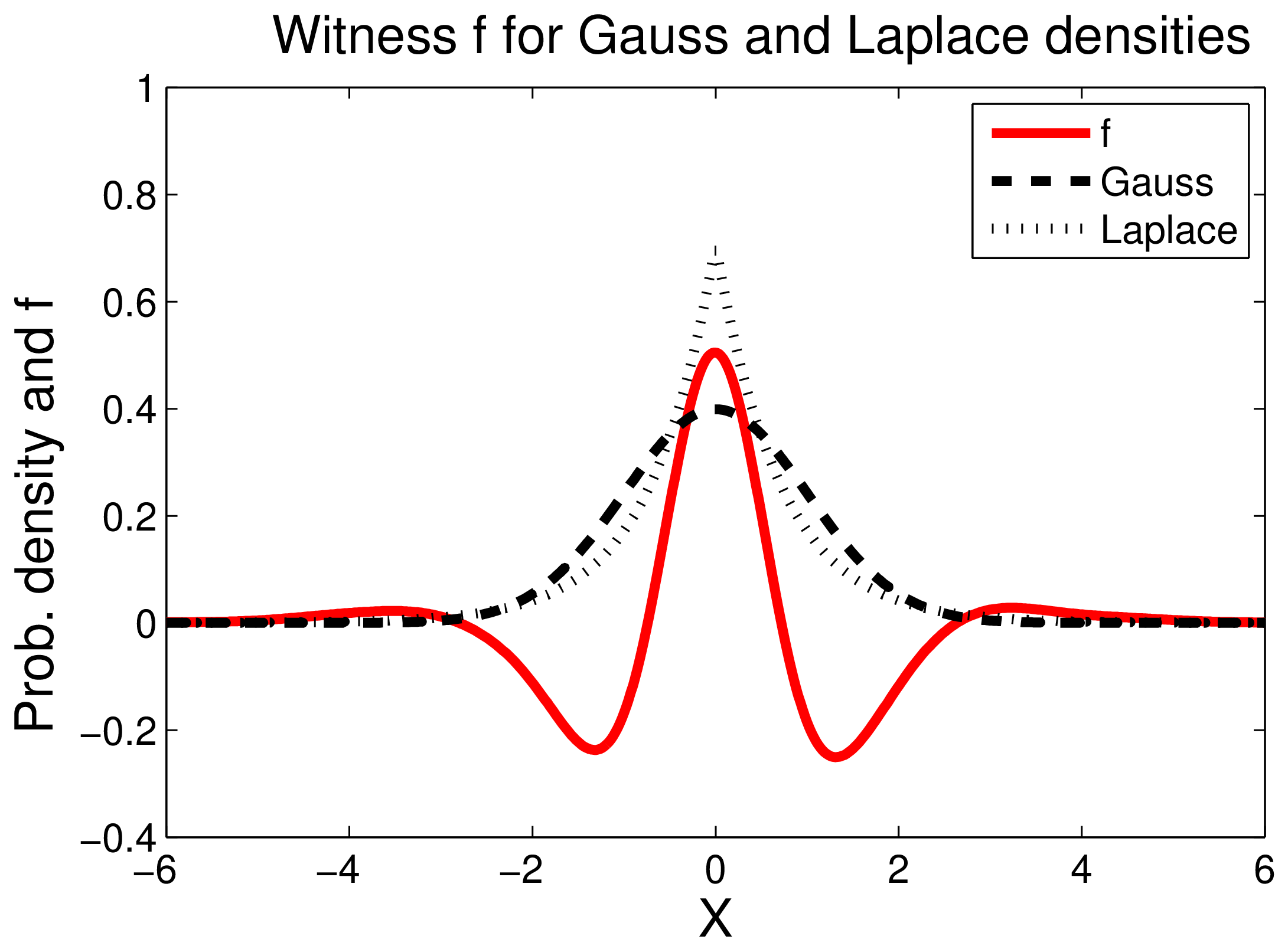
It is also instructive to consider the witness $f$ which is chosen by MMD to exhibit the maximum discrepancy between the two distributions. The population $f$ and its empirical estimate $\hat{f}(x)$ are respectively
$ \begin{array}{cclcl} f(x) &\propto &\left\langle \phi(x),\mu[p] - \mu[q] \right\rangle &= & \mathbf{E}{x' \sim p} \left[k(x,x')\right] - \mathbf{E}{x' \sim q} \left[k(x,x')\right] \ \hat{f}(x) &\propto &\left\langle \phi(x),\mu[X] - \mu[Y] \right\rangle &= &\frac{1}{m} \sum_{i=1}^m k(x_i, x) - \frac{1}{n} \sum_{i=1}^n k(y_i, x). \end{array} $
This follows from the fact that the unit vector $v$ maximizing $\left\langle v,x \right\rangle_{\mathcal{H}}$ in a Hilbert space is $v = x/\left|x\right|$.
We illustrate the behavior of MMD in Figure 1 using a one-dimensional example. The data $X$ and $Y$ were generated from distributions $p$ and $q$ with equal means and variances, with $p$ Gaussian and $q$ Laplacian. We chose $\mathcal{F}$ to be the unit ball in an RKHS using the Gaussian kernel. We observe that the function $f$ that witnesses the MMD — in other words, the function maximizing the mean discrepancy in Equation (1) — is smooth, positive where the Laplace density exceeds the Gaussian density (at the center and tails), and negative where the Gaussian density is larger. Moreover, the magnitude of $f$ is a direct reflection of the amount by which one density exceeds the other, insofar as the smoothness constraint permits it.
2.4 The MMD in Other Function Classes
The definition of the maximum mean discrepancy is by no means limited to RKHS. In fact, any function class $\mathcal{F}$ that comes with uniform convergence guarantees and is sufficiently powerful will enjoy the above properties.
########## {caption="Definition"}
Let $\mathcal{F}$ be a subset of some vector space. The star $S[\mathcal{F}]$ of a set $\mathcal{F}$ is
$ S[\mathcal{F}] := \left{\alpha x | x \in \mathcal{F} \text{ and } \alpha \in [0, \infty)\right} $
########## {caption="Theorem 7"}
Denote by $\mathcal{F}$ the subset of some vector space of functions from $\mathcal{X}$ to $\mathbb{R}$ for which $S[\mathcal{F}] \cap C(\mathcal{X})$ is dense in $C(\mathcal{X})$ with respect to the $L_\infty(\mathcal{X})$ norm. Then $\mathrm{MMD}\left[\mathcal{F}, p,q\right] = 0$ if and only if $p = q$.
Moreover, under the above conditions $\mathrm{MMD}[\mathcal{F}, p, q]$ is a metric on the space of probability distributions. Whenever the star of $\mathcal{F}$ is not dense, $\mathrm{MMD}$ is a pseudo-metric space.[^3]
[^3]: According to [7] p. 26 a metric $d(x,y)$ satisfies the following four properties: symmetry, triangle inequality, $d(x,x)=0$, and $d(x,y)=0\implies x=y$. A pseudo-metric only satisfies the first three properties.
Proof: The first part of the proof is almost identical to that of Theorem 4 and is therefore omitted. To see the second part, we only need to prove the triangle inequality. We have
$ \begin{aligned} \sup_{f \in \mathcal{F}} \left|E_p f - E_q f\right| + \sup_{g \in \mathcal{F}} \left|E_q g - E_r g\right| &\geq \sup_{f \in \mathcal{F}} \left[\left|E_p f - E_q f\right| + \left|E_q f - E_r \right|\right] \ &\geq \sup_{f \in \mathcal{F}} \left|E_p f - E_r f\right|. \end{aligned} $
The first part of the theorem establishes that $\mathrm{MMD}[\mathcal{F}, p, q]$ is a metric, since only for $p = q$ do we have $\mathrm{MMD}[\mathcal{F}, p, q] = 0$.
Note that any uniform convergence statements in terms of $\mathcal{F}$ allow us immediately to characterize an estimator of $\mathrm{MMD}(\mathcal{F}, p, q)$ explicitly. The following result shows how (we will refine this reasoning for the RKHS case in Section 4).
########## {caption="Theorem 8"}
Let $\delta \in (0, 1)$ be a confidence level and assume that for some $\epsilon(\delta, m, \mathcal{F})$ the following holds for samples $\left{x_1, \ldots, x_m\right}$ drawn from $p$:
$ \Pr\left{\sup_{f \in \mathcal{F}} \left| \mathbf{E}p[f] - \frac{1}{m} \sum{i=1}^m f(x_i)\right| > \epsilon(\delta, m, \mathcal{F})\right} \leq \delta. $
In this case we have that
$ \Pr\left{ \left| \mathrm{MMD}[\mathcal{F},p,q] - \mathrm{MMD}_b[\mathcal{F},X,Y]\right| > 2 \epsilon(\delta/2,m, \mathcal{F})\right} \leq \delta. $
Proof: The proof works simply by using convexity and suprema as follows:
$ \begin{aligned} & \left| \mathrm{MMD}[\mathcal{F},p,q] - \mathrm{MMD}b[\mathcal{F},X,Y]\right| \ = & \left|\sup{f \in \mathcal{F}} \left|\mathbf{E}p[f] - \mathbf{E}q[f]\right| - \sup{f \in \mathcal{F}} \left|\frac{1}{m} \sum{i=1}^m f(x_i) - \frac{1}{n} \sum_{i=1}^n f(y_i)\right|\right| \ \leq & \sup_{f \in \mathcal{F}} \left| \mathbf{E}p[f] - \mathbf{E}q[f] - \frac{1}{m} \sum{i=1}^m f(x_i) + \frac{1}{n} \sum{i=1}^n f(y_i)\right| \ \leq & \sup_{f \in \mathcal{F}} \left| \mathbf{E}p[f] - \frac{1}{m} \sum{i=1}^m f(x_i)\right| + \sup_{f \in \mathcal{F}} \left| \mathbf{E}q[f] - \frac{1}{n} \sum{i=1}^n f(y_i)\right|. \end{aligned} $
Bounding each of the two terms via a uniform convergence bound proves the claim.
This shows that $\mathrm{MMD}_b[\mathcal{F}, X, Y]$ can be used to estimate $\mathrm{MMD}[\mathcal{F}, p, q]$ and that the quantity is asymptotically unbiased.
########## {caption="Remark: Reduction to Binary Classification"}
Any classifier which maps a set of observations $\left{z_i, l_i\right}$ with $z_i \in \mathcal{X}$ on some domain $\mathcal{X}$ and labels $l_i \in \left{\pm 1\right}$, for which uniform convergence bounds exist on the convergence of the empirical loss to the expected loss, can be used to obtain a similarity measure on distributions — simply assign $l_i = 1$ if $z_i \in X$ and $l_i = -1$ for $z_i \in Y$ and find a classifier which is able to separate the two sets. In this case maximization of $\mathbf{E}_p[f] - \mathbf{E}_q[f]$ is achieved by ensuring that as many $z \sim p(z)$ as possible correspond to $f(z) = 1$, whereas for as many $z \sim q(z)$ as possible we have $f(z) = -1$. Consequently neural networks, decision trees, boosted classifiers and other objects for which uniform convergence bounds can be obtained can be used for the purpose of distribution comparison. For instance, [13] Section 4 use the error of a hyperplane classifier to approximate the $\mathcal{A}$-distance between distributions of [14].
2.5 Examples of Non-RKHS Function Classes
Other function spaces $\mathcal{F}$ inspired by the statistics literature can also be considered in defining the MMD. Indeed, Lemma 2 defines an MMD with $\mathcal{F}$ the space of bounded continuous real-valued functions, which is a Banach space with the supremum norm ([7] p. 158). We now describe two further metrics on the space of probability distributions, the Kolmogorov-Smirnov and Earth Mover's distances, and their associated function classes.
2.5.1 Kolmogorov-Smirnov Statistic
The Kolmogorov-Smirnov (K-S) test is probably one of the most famous two-sample tests in statistics. It works for random variables $x \in \mathbb{R}$ (or any other set for which we can establish a total order). Denote by $F_p(x)$ the cumulative distribution function of $p$ and let $F_X(x)$ be its empirical counterpart, that is
$ F_p(z) := \Pr\left{x \leq z \text{ for } x \sim p(x)\right} \text{ and } F_X(z) := \frac{1}{|X|} \sum_{i=1}^m 1_{z \leq x_i}. $
It is clear that $F_p$ captures the properties of $p$. The Kolmogorov metric is simply the $L_\infty$ distance $\left|F_X - F_Y\right|_\infty$ for two sets of observations $X$ and $Y$. [15] showed that for $p = q$ the limiting distribution of the empirical cumulative distribution functions satisfies
$ \lim_{m,n \to \infty} \Pr\left{\left[\textstyle \frac{mn}{m+n}\right]^{\frac{1}{2}} \left|F_X - F_Y\right|\infty > x \right} = 2 \sum{j=1}^\infty (-1)^{j-1} e^{-2j^2 x^2} \text{ for } x \geq 0. $
This allows for an efficient characterization of the distribution under the null hypothesis $\mathcal{H}_0$. Efficient numerical approximations to (7) can be found in numerical analysis handbooks ([16]). The distribution under the alternative, $p \neq q$, however, is unknown.
The Kolmogorov metric is, in fact, a special instance of $\mathrm{MMD}[\mathcal{F}, p, q]$ for a certain Banach space ([9] Theorem 5.2)
########## {caption="Proposition 9"}
Let $\mathcal{F}$ be the class of functions $\mathcal{X} \to \mathbb{R}$ of bounded variation[^4]
- Then $\mathrm{MMD}[\mathcal{F}, p, q] = \left|F_p - F_q\right|_\infty$.
[^4]: A function $f$ defined on $[a,b]$ is of bounded variation $C$ if the total variation is bounded by $C$, i.e. the supremum over all sums
$ \sum_{1\le i \le n} |f(x_i) - f(x_{i-1})|, $
where $a\le x_0 \le \ldots \le x_n \le b$ ([7] p. 184).
2.5.2 Earth-Mover Distances
Another class of distance measures on distributions that may be written as an MMD are the Earth-Mover distances. We assume $(\mathcal{X},d)$ is a separable metric space, and define $\mathcal{P}{1}(\mathcal{X})$ to be the space of probability measures on $\mathcal{X}$ for which $\int d(x,z)dp(z)<\infty$ for all $p\in\mathcal{P}{1}(\mathcal{X})$ and $x\in\mathcal{X}$ (these are the probability measures for which $\mathbf{E}\left|x\right|<\infty$ when $\mathcal{X}= \mathbb{R}$). We then have the following definition ([7] p. 420).
########## {caption="Definition: Monge-Wasserstein metric"}
Let $p\in\mathcal{P}{1}(\mathcal{X})$ and $q\in\mathcal{P}{1}(\mathcal{X})$. The Monge-Wasserstein distance is defined as
$ W(p,q):=\inf_{\mu\in M(p,q)}\int d(x,y)d\mu(x,y), $
where $M(p,q)$ is the set of joint distributions on $\mathcal{X}\times\mathcal{X}$ with marginals $p$ and $q$.
We may interpret this as the cost (as represented by the metric $d(x,y)$) of transferring mass distributed according to $p$ to a distribution in accordance with $q$, where $\mu$ is the movement schedule. In general, a large variety of costs of moving mass from $x$ to $y$ can be used, such as psychooptical similarity measures in image retrieval ([17]). The following theorem holds ([7] Theorem 11.8.2).
########## {caption="Theorem 10: Kantorovich-Rubinstein"}
Let $p\in\mathcal{P}{1}(\mathcal{X})$ and $q\in\mathcal{P}{1}(\mathcal{X})$, where $\mathcal{X}$ is separable. Then a metric on $\mathcal{P}_{1}(S)$ is defined as
$ W(p,q)=\left\Vert p-q\right\Vert {L}^{*}=\sup{\left\Vert f\right\Vert _{L}\le1}\left|\int f, d(p-q)\right|, $
where
$ \left\Vert f\right\Vert {L}:=\sup{x\neq y,\in, \mathcal{X}}\frac{\left|f(x)-f(y)\right|}{d(x,y)} $
is the Lipschitz seminorm [^5] for real valued $f$ on $\mathcal{X}$.
[^5]: A seminorm satisfies the requirements of a norm besides $\left\Vert x\right\Vert =0$ only for $x=0$ ([7] p. 156).
A simple example of this theorem is as follows ([7] Exercise 1, p. 425).
########## {caption="Example"}
Let $\mathcal{X}= \mathbb{R}$ with associated $d(x,y)=\left|x-y\right|$. Then given $f$ such that $\left\Vert f\right\Vert _{L}\le1$, we use integration by parts to obtain
$ \left|\int f, d(p-q)\right|=\left|\int(F_{p}-F_{q})(x)f'(x)dx\right|\le\int\left|(F_{p}-F_{q})\right|(x)dx, $
where the maximum is attained for the function $g$ with derivative $g'=2, 1_{F_{p}>F_{q}}-1$ (and for which $\left\Vert g\right\Vert {L}=1$). We recover the $L{1}$ distance between distribution functions,
$ W(P,Q)=\int\left|(F_{p}-F_{q})\right|(x)dx. $
One may further generalize Theorem 10 to the set of all laws $\mathcal{P}(\mathcal{X})$ on arbitrary metric spaces $\mathcal{X}$ ([7] Proposition 11.3.2).
########## {caption="Definition: Bounded Lipschitz metric"}
Let $p$ and $q$ be laws on a metric space $\mathcal{X}$. Then
$ \beta(p,q):=\sup_{\left\Vert f\right\Vert _{BL}\le1}\left|\int f, d(p-q)\right| $
is a metric on $\mathcal{P}(\mathcal{X})$, where $f$ belongs to the space of bounded Lipschitz functions with norm
$ \left\Vert f\right\Vert _{BL}:=\left\Vert f\right\Vert _{L}+\left\Vert f\right\Vert _{\infty}. $
3. Background Material
Section Summary: The section introduces key concepts from statistical hypothesis testing, including the null hypothesis that two distributions are identical, the risks of Type I and Type II errors, and the role of a significance level in setting decision thresholds for a test statistic such as the MMD. It then presents an example demonstrating that no test can reliably distinguish certain pairs of distributions at any fixed sample size without additional assumptions, because one distribution can be constructed to mimic the other with high probability. Finally, it briefly surveys earlier multivariate two-sample methods, such as generalizations of runs tests and Kolmogorov-Smirnov procedures based on minimum spanning trees or matchings.
We now present three background results. First, we introduce the terminology used in statistical hypothesis testing. Second, we demonstrate via an example that even for tests which have asymptotically no error, one cannot guarantee performance at any fixed sample size without making assumptions about the distributions. Finally, we briefly review some earlier approaches to the two-sample problem.
3.1 Statistical Hypothesis Testing
Having described a metric on probability distributions (the MMD) based on distances between their Hilbert space embeddings, and empirical estimates (biased and unbiased) of this metric, we now address the problem of determining whether the empirical MMD shows a statistically significant difference between distributions. To this end, we briefly describe the framework of statistical hypothesis testing as it applies in the present context, following [18], Chapter 8. Given i.i.d. samples $X\sim p$ of size $m$ and $Y\sim q$ of size $n$, the statistical test, $\mathcal{T}(X,Y),:, \mathcal{X}^m \times \mathcal{X}^n\mapsto{0,1}$ is used to distinguish between the null hypothesis $\mathcal{H}_0,:,p=q$ and the alternative hypothesis $\mathcal{H}_1,:,p\neq q$. This is achieved by comparing the test statistic[^6] $\mathrm{MMD}[\mathcal{F},X,Y]$ with a particular threshold: if the threshold is exceeded, then the test rejects the null hypothesis (bearing in mind that a zero population MMD indicates $p=q$). The acceptance region of the test is thus defined as the set of real numbers below the threshold. Since the test is based on finite samples, it is possible that an incorrect answer will be returned: we define the Type I error as the probability of rejecting $p=q$ based on the observed sample, despite the null hypothesis having generated the data. Conversely, the Type II error is the probability of accepting $p=q$ despite the underlying distributions being different. The level $\alpha$ of a test is an upper bound on the Type I error: this is a design parameter of the test, and is used to set the threshold to which we compare the test statistic (finding the test threshold for a given $\alpha$ is the topic of Section 4 and Section 5). A consistent test achieves a level $\alpha$, and a Type II error of zero, in the large sample limit. We will see that the tests proposed in this paper are consistent.
[^6]: This may be biased or unbiased.
3.2 A Negative Result
Even if a test is consistent, it is not possible to distinguish distributions with high probability at a given, fixed sample size (i.e., to provide guarantees on the Type II error), without prior assumptions as to the nature of the difference between $p$ and $q$. This is true regardless of the two-sample test used. There are several ways to illustrate this, which each give different insight into the kinds of differences that might be undetectable for a given number of samples. The following example[^7] is one such illustration.
[^7]: This is a variation of a construction for independence tests, which was suggested in a private communication by John Langford.
########## {caption="Example"}
Assume that we have a distribution $p$ from which we draw $m$ iid observations. Moreover, we construct a distribution $q$ by drawing $m^2$ iid observations from p and subsequently defining a discrete distribution over these $m^2$ instances with probability $m^{-2}$ each. It is easy to check that if we now draw $m$ observations from $q$, there is at least a ${{m^2} \choose m} \frac{m!}{m^{2m}} > 1-e^{-1} > 0.63$ probability that we thereby will have effectively obtained an $m$ sample from $p$. Hence no test will be able to distinguish samples from $p$ and $q$ in this case. We could make the probability of detection arbitrarily small by increasing the size of the sample from which we construct $q$.
3.3 Previous Work
We next give a brief overview of some earlier approaches to the two sample problem for multivariate data. Since our later experimental comparison is with respect to certain of these methods, we give abbreviated algorithm names in italics where appropriate: these should be used as a key to the tables in Section 8. A generalisation of the Wald-Wolfowitz runs test to the multivariate domain was proposed and analysed by [19, 20] (FR Wolf), and involves counting the number of edges in the minimum spanning tree over the aggregated data that connect points in $X$ to points in $Y$. The resulting test relies on the asymptotic normality of the test statistic, and this quantity is not distribution-free under the null hypothesis for finite samples (it depends on $p$ and $q$). The computational cost of this method using Kruskal's algorithm is $O((m+n)^2\log(m+n))$, although more modern methods improve on the $\log(m+n)$ term. See [21] for details. [19] claim that calculating the matrix of distances, which costs $O((m+n)^2)$, dominates their computing time; we return to this point in our experiments (Section 8). Two possible generalisations of the Kolmogorov-Smirnov test to the multivariate case were studied in [22, 19]. The approach of Friedman and Rafsky (FR Smirnov) in this case again requires a minimal spanning tree, and has a similar cost to their multivariate runs test.
A more recent multivariate test was introduced by [23]. This entails computing the minimum distance non-bipartite matching over the aggregate data, and using the number of pairs containing a sample from both $X$ and $Y$ as a test statistic. The resulting statistic is distribution-free under the null hypothesis at finite sample sizes, in which respect it is superior to the Friedman-Rafsky test; on the other hand, it costs $O((m+n)^3)$ to compute. Another distribution-free test (Hall) was proposed by [24]: for each point from $p$, it requires computing the closest points in the aggregated data, and counting how many of these are from $q$ (the procedure is repeated for each point from $q$ with respect to points from $p$). As we shall see in our experimental comparisons, the test statistic is costly to compute; [24] consider only tens of points in their experiments.
Yet another approach is to use some distance (e.g. $L_1$ or $L_2$) between Parzen window estimates of the densities as a test statistic ([25, 26]), based on the asymptotic distribution of this distance given $p=q$. When the $L_2$ norm is used, the test statistic is related to those we present here, although it is arrived at from a different perspective. Briefly, the test of [25] is obtained in a more restricted setting where the RKHS kernel is an inner product between Parzen windows. Since we are not doing density estimation, however, we need not decrease the kernel width as the sample grows. In fact, decreasing the kernel width reduces the convergence rate of the associated two-sample test, compared with the $(m + n)^{-1/2}$ rate for fixed kernels. We provide more detail in Section 7.1. The $L_1$ approach of [26] (Biau) requires the space to be partitioned into a grid of bins, which becomes difficult or impossible for high dimensional problems. Hence we use this test only for low-dimensional problems in our experiments.
4. Tests Based on Uniform Convergence Bounds
Section Summary: This section presents two hypothesis tests for determining whether two finite samples come from the same underlying distribution, each equipped with explicit guarantees on error rates that hold for any sample size. The tests derive decision thresholds from concentration inequalities that bound how far an empirical estimate of distribution difference can stray from its true value under the null hypothesis of equality, with one version based on a biased statistic and the other on an unbiased variant. These bounds also establish that both procedures are consistent, so the chance of mistakenly accepting unequal distributions shrinks at a predictable rate as more data arrive.
In this section, we introduce two statistical tests of independence which have exact performance guarantees at finite sample sizes, based on uniform convergence bounds. The first, in Section 4.1, uses the [27] bound on the biased MMD statistic, and the second, in Section 4.2, uses a [28] bound for the unbiased statistic.
4.1 Bound on the Biased Statistic and Test
We establish two properties of the MMD, from which we derive a hypothesis test. First, we show that regardless of whether or not $p=q$, the empirical MMD converges in probability at rate $O((m+n)^{-\frac{1}{2}})$ to its population value. This shows the consistency of statistical tests based on the MMD. Second, we give probabilistic bounds for large deviations of the empirical MMD in the case $p=q$. These bounds lead directly to a threshold for our first hypothesis test. We begin our discussion of the convergence of $\mathrm{MMD}_b[\mathcal{F}, X, Y]$ to $\mathrm{MMD}[\mathcal{F}, p,q]$.
########## {caption="Theorem 11"}
Let $p,q,X,Y$ be defined as in Problem 1, and assume $0\le k(x,y)\le K$. Then
$ \Pr\left{\left| \mathrm{MMD}_b[\mathcal{F}, X,Y] - \mathrm{MMD}[\mathcal{F}, p, q]\right| > 2\left( (K/m)^{\frac{1}{2}} + (K/n)^{\frac{1}{2}} \right) + \epsilon\right} \leq 2\exp\left(\textstyle \frac{-\epsilon^2 m n}{2 K (m+n)}\right). $
See Appendix A.2 for proof. Our next goal is to refine this result in a way that allows us to define a test threshold under the null hypothesis $p=q$. Under this circumstance, the constants in the exponent are slightly improved.
########## {caption="Theorem 12"}
Under the conditions of Theorem 11 where additionally $p = q$ and $m = n$,
$ \nonumber \mathrm{MMD}_b[\mathcal{F}, X,Y] \leq \underset{B_1(\mathcal{F},p)} {\underbrace{ m^{-\frac{1}{2}} \sqrt{2 \mathbf{E}_p\left[k(x,x) - k(x,x')\right]}}}
- \epsilon \leq \underset{B_2(\mathcal{F},p)} {\underbrace{ (2K/m)^{1/2}}}
- \epsilon, $
both with probability at least $1-\exp\left(-\frac{\epsilon^2 m}{4 K}\right)$ (see Appendix A.3 for the proof).
In this theorem, we illustrate two possible bounds $B_1(\mathcal{F},p)$ and $B_2(\mathcal{F},p)$ on the bias in the empirical estimate Equation (6). The first inequality is interesting inasmuch as it provides a link between the bias bound $B_1(\mathcal{F},p)$ and kernel size (for instance, if we were to use a Gaussian kernel with large $\sigma$, then $k(x,x)$ and $k(x,x')$ would likely be close, and the bias small). In the context of testing, however, we would need to provide an additional bound to show convergence of an empirical estimate of $B_1(\mathcal{F},p)$ to its population equivalent. Thus, in the following test for $p=q$ based on Theorem 12, we use $B_2(\mathcal{F},p)$ to bound the bias.[^8]
[^8]: Note that we use a tighter bias bound than [2].
########## {caption="Corollary 13"}
A hypothesis test of level $\alpha$ for the null hypothesis $p=q$, that is, for $\mathrm{MMD}[\mathcal{F}, p,q] =0$, has the acceptance region $\mathrm{MMD}_b[\mathcal{F}, X,Y] < \sqrt{2K/m} \left( 1 + \sqrt{2\log \alpha^{-1}} \right).$
We emphasise that Theorem 11 guarantees the consistency of the test, and that the Type II error probability decreases to zero at rate $O(m^{-\frac{1}{2}})$, assuming $m=n$. To put this convergence rate in perspective, consider a test of whether two normal distributions have equal means, given they have unknown but equal variance ([18], Exercise 8.41). In this case, the test statistic has a Student-$t$ distribution with $n+m-2$ degrees of freedom, and its error probability converges at the same rate as our test.
It is worth noting that bounds may be obtained for the deviation between expectations $\mu[p]$ and the empirical means $\mu[X]$ in a completely analogous fashion. The proof requires symmetrization by means of a ghost sample, i.e. a second set of observations drawn from the same distribution. While not the key focus of the present paper, such bounds can be used in the design of inference principles based on moment matching [29, 30, 31].
4.2 Bound on the Unbiased Statistic and Test
While the previous bounds are of interest since the proof strategy can be used for general function classes with well behaved Rademacher averages, a much easier approach may be used directly on the unbiased statistic $\mathrm{MMD}_{u}^{2}$ in Lemma 5. We base our test on the following theorem, which is a straightforward application of the large deviation bound on U-statistics of [28] p. 25.
########## {caption="Theorem 14"}
Assume $0\le k(x_{i},x_{j})\le K$, from which it follows $-2K\le h(z_{i},z_{j})\le2K$. Then
$ \Pr\left{ \mathrm{MMD}_{u}^{2}(\mathcal{F},X,Y)-\mathrm{MMD}^{2}(\mathcal{F},p,q)>t\right} \le\exp\left(\frac{-t^{2}m_2}{8 K^{2}}\right) $
where $m_2 := \lfloor m/2 \rfloor$ (the same bound applies for deviations of $-t$ and below).
A consistent statistical test for $p=q$ using $\mathrm{MMD}_{u}^{2}$ is then obtained.
########## {caption="Corollary 15"}
A hypothesis test of level $\alpha$ for the null hypothesis $p=q$ has the acceptance region $\mathrm{MMD}_{u}^{2} < \left(4K/\sqrt{m}\right)\sqrt{\log(\alpha^{-1})}$.
We now compare the thresholds of the two tests. We note first that the threshold for the biased statistic applies to an estimate of $\mathrm{MMD}$, whereas that for the unbiased statistic is for an estimate of $\mathrm{MMD}^2$. Squaring the former threshold to make the two quantities comparable, the squared threshold in Corollary 13 decreases as $m^{-1}$, whereas the threshold in Corollary 15 decreases as $m^{-1/2}$. Thus for sufficiently large[^9] $m$, the McDiarmid-based threshold will be lower (and the associated test statistic is in any case biased upwards), and its Type II error will be better for a given Type I bound. This is confirmed in our Section 8 experiments. Note, however, that the rate of convergence of the squared, biased MMD estimate to its population value remains at $1/\sqrt{m}$ (bearing in mind we take the square of a biased estimate, where the bias term decays as $1/\sqrt{m}$).
[^9]: In the case of $\alpha=0.05$, this is $m\ge 12$.
Finally, we note that the bounds we obtained here are rather conservative for a number of reasons: first, they do not take the actual distributions into account. In fact, they are finite sample size, distribution free bounds that hold even in the worst case scenario. The bounds could be tightened using localization, moments of the distribution, etc. Any such improvements could be plugged straight into Theorem 8 for a tighter bound. See e.g. [32] for a detailed discussion of recent uniform convergence bounding methods. Second, in computing bounds rather than trying to characterize the distribution of $\mathrm{MMD}(\mathcal{F}, X,Y)$ explicitly, we force our test to be conservative by design. In the following we aim for an exact characterization of the asymptotic distribution of $\mathrm{MMD}(\mathcal{F}, X, Y)$ instead of a bound. While this will not satisfy the uniform convergence requirements, it leads to superior tests in practice.
5. Test Based on the Asymptotic Distribution of the Unbiased Statistic
Section Summary: This section introduces a hypothesis test for whether two distributions are identical, relying on the large-sample behavior of an unbiased estimator of the maximum mean discrepancy (MMD). When the distributions differ, the scaled estimator converges to a normal distribution whose variance can be estimated from the data; when they are the same, it follows a weighted sum of centered chi-squared variables whose weights come from the eigenvalues of a centered kernel operator. The resulting test compares the observed statistic against a critical value obtained either by bootstrapping the pooled samples or by matching the first three moments to a Pearson curve, with a simple correction ensuring the estimator remains practically nonnegative.
We now propose a third test, which is based on the asymptotic distribution of the unbiased estimate of $\mathrm{MMD}^2$ in Lemma 6.
########## {caption="Theorem 16"}
We assume $\mathbf{E}\left( h^2 \right)<\infty$. Under $\mathcal{H}_1$, $\mathrm{MMD}_u^2$ converges in distribution (see e.g. [33] Section 7.2) to a Gaussian according to
$ m^{\frac{1}{2}}\left( \mathrm{MMD}^2_u - \mathrm{MMD}^2\left[\mathcal{F},p,q\right] \right) \overset{D}{\rightarrow} \mathcal{N}\left(0, \sigma^2_u \right), : $
where $\sigma^2_u = 4 \left( \mathbf{E}{z} \left[ (\mathbf{E}{z'} h(z,z') )^2 \right] - \left[ \mathbf{E}_{z,z'} ( h(z,z') ) \right]^2 \right)$, uniformly at rate $1/\sqrt{m}$ ([11], Theorem B, p. 193). Under $\mathcal{H}0$, the U-statistic is degenerate, meaning $\mathbf{E}{z'}h(z,z')=0$. In this case, $\mathrm{MMD}_u^2$ converges in distribution according to
$ m \mathrm{MMD}u^2 \overset{D}{\rightarrow} \sum{l=1}^{\infty} \lambda_l \left[ z_l^2 - 2 \right], $
where $z_l\sim \mathcal{N}(0,2)$ i.i.d., $\lambda_i$ are the solutions to the eigenvalue equation
$ \int_{\mathcal{X}} \tilde{k}(x,x') \psi_{i}(x)dp(x)=\lambda_{i}\psi_{i}(x'), $
and $\tilde{k}(x_{i},x_{j}):=k(x_{i},x_{j})-\mathbf{E}{x}k(x{i},x)-\mathbf{E}{x}k(x,x{j})+\mathbf{E}_{x,x'}k(x,x')$ is the centred RKHS kernel.
The asymptotic distribution of the test statistic under $\mathcal{H}_1$ is given by [11] Section 5.5.1, and the distribution under $\mathcal{H}_0$ follows [11] Section 5.5.2 and [25] Appendix; see Appendix B.1 for details. We illustrate the MMD density under both the null and alternative hypotheses by approximating it empirically for both $p=q$ and $p\neq q$. Results are plotted in Figure 2.
:::: {.figure cols="2"}
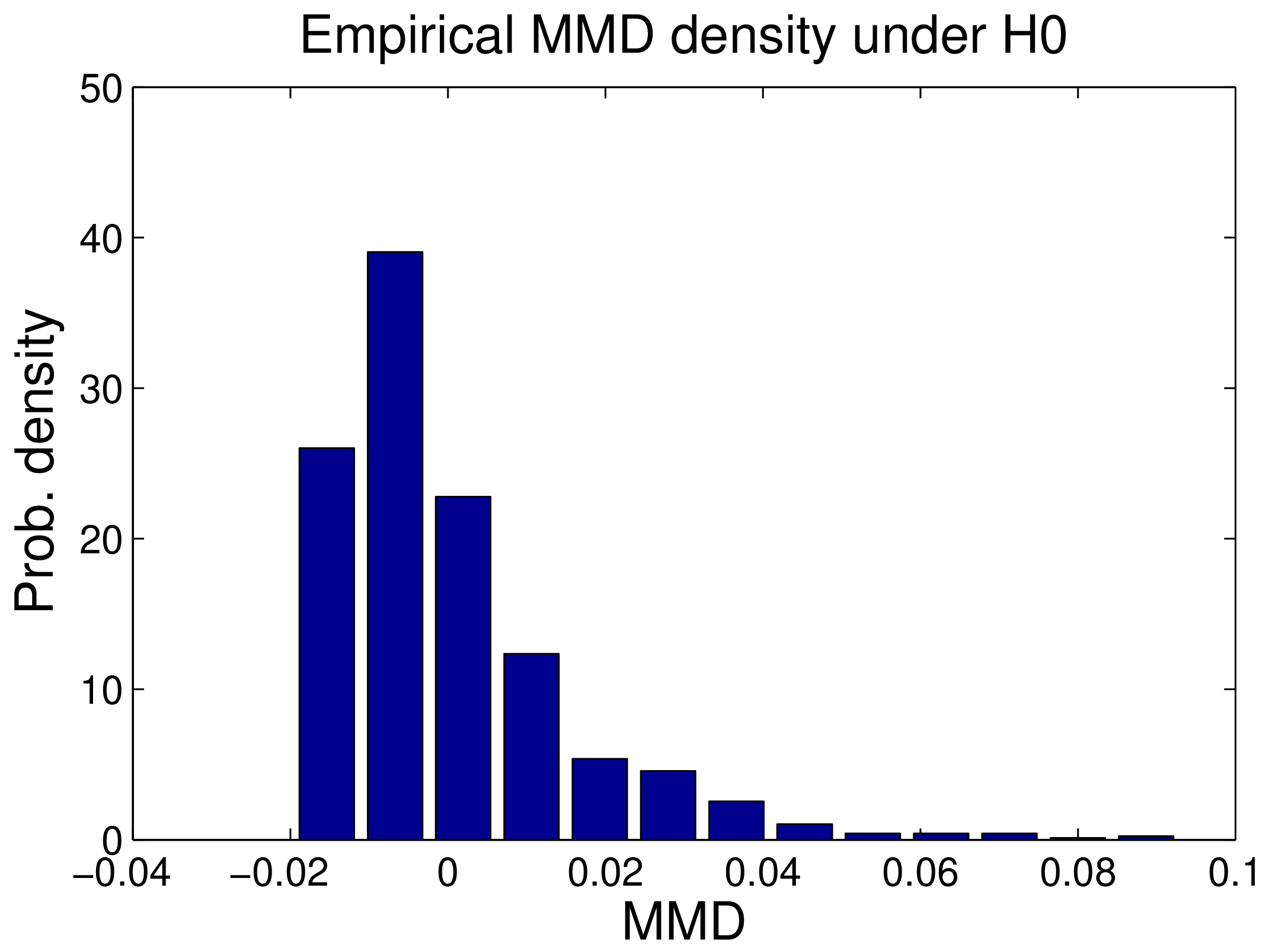
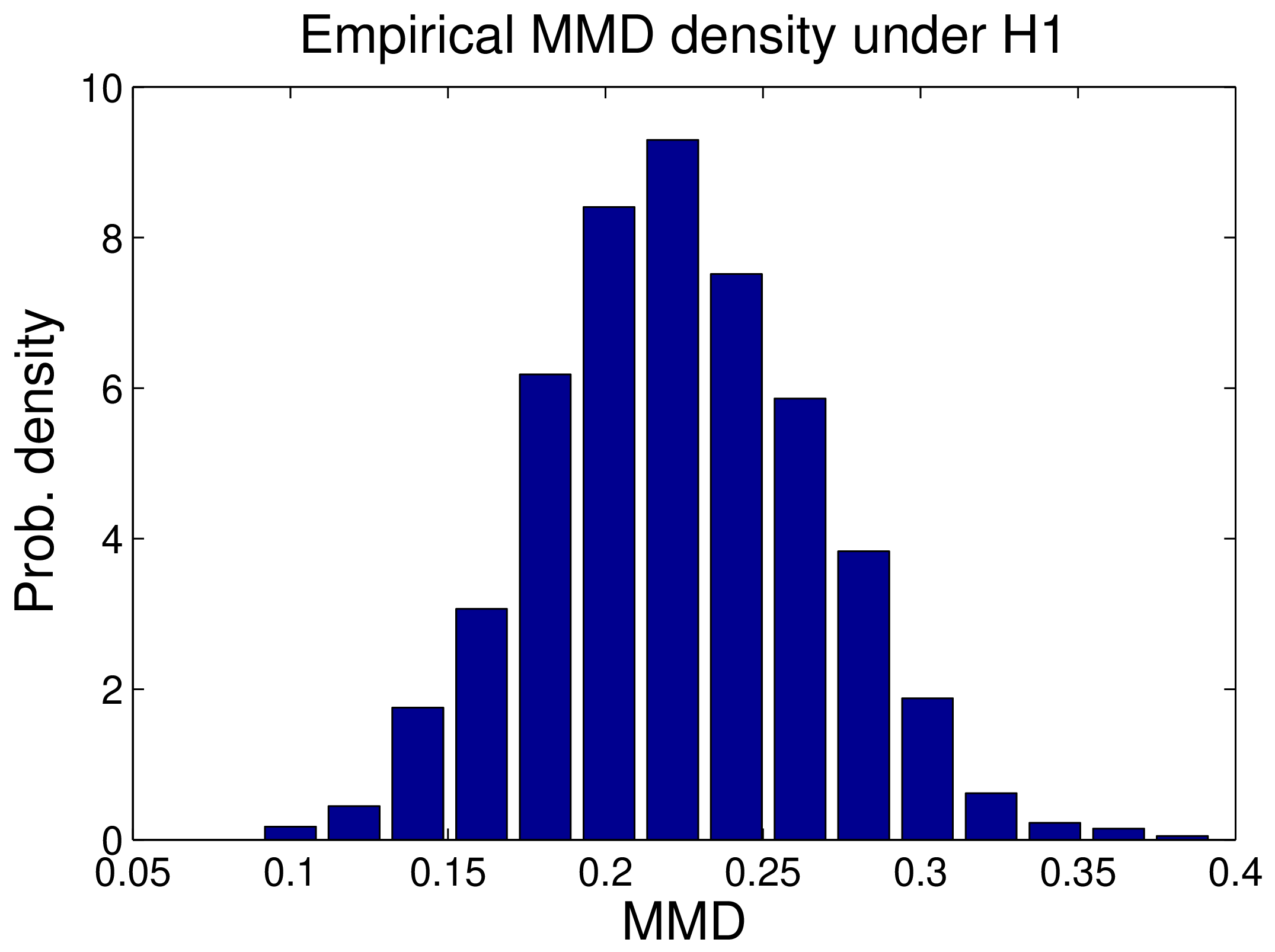
Figure 2: Left: Empirical distribution of the MMD under $\mathcal{H}_0$, with $p$ and $q$ both Gaussians with unit standard deviation, using 50 samples from each. Right: Empirical distribution of the MMD under $\mathcal{H}_1$, with $p$ a Laplace distribution with unit standard deviation, and $q$ a Laplace distribution with standard deviation $3 \sqrt{2}$, using 100 samples from each. In both cases, the histograms were obtained by computing 2000 independent instances of the MMD. ::::
Our goal is to determine whether the empirical test statistic $\mathrm{MMD}_u^2$ is so large as to be outside the $1-\alpha$ quantile of the null distribution in Equation (8) (consistency of the resulting test is guaranteed by the form of the distribution under $\mathcal{H}_1$). One way to estimate this quantile is using the bootstrap on the aggregated data, following [34]. Alternatively, we may approximate the null distribution by fitting Pearson curves to its first four moments ([35], Section 18.8). Taking advantage of the degeneracy of the U-statistic, we obtain (see Appendix B.2)
$ \begin{aligned} \mathbf{E}\left(\left[\mathrm{MMD}u^2\right]^2\right) & = \frac{2}{m(m-1)}\mathbf{E}{z,z'}\left[h^{2}(z,z') \right] \text{ and } \ \mathbf{E}\left(\left[\mathrm{MMD}u^2\right]^3\right) & = \frac{8(m-2)}{m^{2}(m-1)^{2}}\mathbf{E}{z,z'}\left[h(z,z')\mathbf{E}_{z''}\left(h(z,z'')h(z',z'')\right)\right]
- O(m^{-4}). \end{aligned} $
The fourth moment $\mathbf{E}\left(\left[\mathrm{MMD}_u^2\right]^4\right)$ is not computed, since it is both very small, $O(m^{-4})$, and expensive to calculate, $O(m^4)$. Instead, we replace the kurtosis[^10] with a lower bound due to [36], $\mathrm{kurt}\left(\mathrm{MMD}^2_u\right)\ge \left(\mathrm{skew}\left(\mathrm{MMD}^2_u\right)\right)^2+1$.
[^10]: The kurtosis is defined in terms of the fourth and second moments as $\mathrm{kurt}\left(\mathrm{MMD}^2_u\right) = \frac{\mathbf{E}\left(\left[\mathrm{MMD}_u^2\right]^4\right)}{\left[\mathbf{E}\left(\left[\mathrm{MMD}_u^2\right]^2\right)\right]^2} -3$.
Note that $\mathrm{MMD}^2_u$ may be negative, since it is an unbiased estimator of $(\mathrm{MMD}[\mathcal{F},p,q])^2$. However, the only terms missing to ensure nonnegativity are the terms $h(z_i, z_i)$, which were removed to remove spurious correlations between observations. Consequently we have the bound
$ \mathrm{MMD}u^2 + \frac{1}{m(m-1)} \sum{i=1}^m k(x_i, x_i) + k(y_i, y_i)
- 2k(x_i, y_i) \geq 0. $
6. A Linear Time Statistic and Test
Section Summary: The section introduces a linear-time estimator for the maximum mean discrepancy that works by randomly pairing samples from two datasets and averaging a kernel function over those pairs, yielding an unbiased statistic that needs only constant memory and runs in a single pass. This makes the test practical for streaming data while still allowing standard concentration bounds and a central-limit result to set decision thresholds. The authors note that the approach trades some statistical efficiency for speed and briefly mention low-rank matrix approximations as another possible route to lower cost.
While the above tests are already more efficient than the $O(m^2 \log m)$ and $O(m^3)$ tests described earlier, it is still desirable to obtain $O(m)$ tests which do not sacrifice too much statistical power. Moreover, we would like to obtain tests which have $O(1)$ storage requirements for computing the test statistic in order to apply it to data streams. We now describe how to achieve this by computing the test statistic based on a subsampling of the terms in the sum. The empirical estimate in this case is obtained by drawing pairs from $X$ and $Y$ respectively without replacement.
########## {caption="Lemma"}
Recall $m_2 := \lfloor m/2 \rfloor$. The estimator
$ \mathrm{MMD}l^2[\mathcal{F}, X, Y] := \frac{1}{m_2} \sum{i=1}^{m_2} h((x_{2i-1}, y_{2i-1}), (x_{2i}, y_{2i})) $
can be computed in linear time. Moreover, it is an unbiased estimate of $\mathrm{MMD}^2[\mathcal{F}, p, q]$.
While it is expected (as we will see explicitly later) that $\mathrm{MMD}_l^2$ has higher variance than $\mathrm{MMD}_u^2$, it is computationally much more appealing. In particular, the statistic can be used in stream computations with need for only $O(1)$ memory, whereas $\mathrm{MMD}_u^2$ requires $O(m)$ storage and $O(m^2)$ time to compute the kernel $h$ on all interacting pairs.
Since $\mathrm{MMD}_l^2$ is just the average over a set of random variables, Hoeffding's bound and the central limit theorem readily allow us to provide both uniform convergence and asymptotic statements for it with little effort. The first follows directly from [28] Theorem 2.
########## {caption="Theorem 17"}
Assume $0\le k(x_i,x_j)\le K$. Then
$ \Pr\left{ \mathrm{MMD}_{l}^{2}(\mathcal{F},X,Y)-\mathrm{MMD}^{2}(\mathcal{F},p,q)>t\right} \le\exp\left(\frac{-t^{2}m_2}{8 K^{2}}\right) $
where $m_2 := \lfloor m/2 \rfloor$ (the same bound applies for deviations of $-t$ and below).
Note that the bound of Theorem 14 is identical to that of Theorem 17, which shows the former is rather loose. Next we invoke the central limit theorem.
########## {caption="Corollary 18"}
Assume $0< \mathbf{E}\left( h^2 \right)<\infty$. Then $\mathrm{MMD}_l^2$ converges in distribution to a Gaussian according to
$ m^{\frac{1}{2}}\left( \mathrm{MMD}^2_l - \mathrm{MMD}^2\left[\mathcal{F},p,q\right] \right) \overset{D}{\rightarrow} \mathcal{N}\left(0, \sigma^2_l \right), $
where $\sigma^2_l = 2 \left[\mathbf{E}{z,z'} h^2(z,z') - \left[ \mathbf{E}{z,z'} h(z,z') \right]^2\right]$, uniformly at rate $1/\sqrt{m}$.
The factor of $2$ arises since we are averaging over only $\lfloor m/2\rfloor$ observations. Note the difference in the variance between Theorem 16 and Corollary 18, namely in the former case we are interested in the average conditional variance $\mathbf{E}{z} {\mathrm{Var}}{z'}[h(z,z')|z]$, whereas in the latter case we compute the full variance ${\mathrm{Var}}_{z,z'}[h(z,z')]$.
We end by noting another potential approach to reducing the computational cost of the MMD, by computing a low rank approximation to the Gram matrix ([37, 38, 39]). An incremental computation of the MMD based on such a low rank approximation would require $O(md)$ storage and $O(m d)$ computation (where $d$ is the rank of the approximate Gram matrix which is used to factorize both matrices) rather than $O(m)$ storage and $O(m^2)$ operations. That said, it remains to be determined what effect this approximation would have on the distribution of the test statistic under $\mathcal{H}_0$, and hence on the test threshold.
7. Similarity Measures Related to MMD
Section Summary: The section explains how the maximum mean discrepancy (MMD) statistic for comparing two distributions connects to several existing similarity measures. It shows that the squared L2 distance between Parzen-window density estimates is a special case of a biased MMD, yet yields slower convergence and performs poorly in high dimensions. The discussion further links MMD to set kernels used in multi-instance learning and to kernel-based tests of independence between random variables.
Our main point is to propose a new kernel statistic to test whether two distributions are the same. However, it is reassuring to observe links to other measures of similarity between distributions.
7.1 Link with $L_2$ Distance between Parzen Window Estimates
In this section, we demonstrate the connection between our test statistic and the Parzen window-based statistic of [25]. We show that a two-sample test based on Parzen windows converges more slowly than an RKHS-based test, also following [25]. Before proceeding, we motivate this discussion with a short overview of the Parzen window estimate and its properties ([40]). We assume a distribution $p$ on $\mathbb{R}^{d}$, which has an associated density function also written $p$ to minimise notation. The Parzen window estimate of this density from an i.i.d. sample $X$ of size $m$ is
$ \nonumber \hat{p}(x) =\frac{1}{m}\sum_{l=1}^{m}\kappa\left(x_{l}-x\right) \text{ where }\kappa\text{ satisfies } \int_{\mathcal{X}}\kappa\left(x\right)dx =1 \text{ and } \kappa\left(x\right)\ge0. $
We may rescale $\kappa$ according to $\frac{1}{h_{m}^{d}}\kappa\left(\frac{x}{h_{m}}\right)$. Consistency of the Parzen window estimate requires
$ \lim_{m\rightarrow\infty}h_{m}^{d}=0\quad\mathrm{and}\quad\lim_{m\rightarrow\infty}mh_{m}^{d}=\infty. $
We now show that the $L_2$ distance between Parzen windows density estimates ([25]) is a special case of the biased MMD in equation (6). Denote by $D_r(p,q) := \left|p-q\right|_r$ the $L_r$ distance. For $r = 1$ the distance $D_r(p,q)$ is known as the Levy distance [41], and for $r = 2$ we encounter distance measures derived from the Renyi entropy [42].
Assume that $\hat{p}$ and $\hat{q}$ are given as kernel density estimates with kernel $\kappa(x-x')$, that is, $\hat{p}(x) = m^{-1} \sum_i \kappa(x_i- x)$ and $\hat{q}(y)$ is defined by analogy. In this case
$ \begin{aligned} D_2(\hat{p},\hat{q})^2 & = \int \left[\frac 1m \sum_i \kappa(x_i- z) - \frac 1n \sum_i \kappa(y_i- z)\right]^2 dz & \ & = \frac 1{m^2} \sum_{i,j=1}^m k(x_i- x_j) + \frac 1{n^2} \sum_{i,j=1}^n k(y_i- y_j)
- \frac 2{mn} \sum_{i,j=1}^{m,n} k(x_i- y_j), & \end{aligned} $
where $k(x-y) = \int \kappa(x-z) \kappa(y-z) dz$. By its definition $k(x-y)$ is a Mercer kernel ([43]), as it can be viewed as inner product between $\kappa(x-z)$ and $\kappa(y-z)$ on the domain $\mathcal{X}$.
A disadvantage of the Parzen window interpretation is that when the Parzen window estimates are consistent (which requires the kernel size to decrease with increasing sample size), the resulting two-sample test converges more slowly than using fixed kernels. According to [25], p. 43, the Type II error of the two-sample test converges as $m^{-1/2}h_m^{-d/2}$. Thus, given the schedule for the Parzen window size decrease in Equation (11), the convergence rate will lie in the open interval $(0,1/2)$: the upper limit is approached as $h_{m}$ decreases more slowly, and the lower limit corresponds to $h_{m}$ decreasing near the upper bound of $1/m$. In other words, by avoiding density estimation, we obtain a better convergence rate (namely $m^{-1/2}$) than using a Parzen window estimate with any permissible bandwidth decrease schedule. In addition, the Parzen window interpretation cannot explain the excellent performance of MMD based tests in experimental settings where the dimensionality greatly exceeds the sample size (for instance the Gaussian toy example in Figure 4 B, for which performance actually improves when the dimensionality increases; and the microarray datasets in Table 1). Finally, our tests are able to employ universal kernels that cannot be written as inner products between Parzen windows, normalized or otherwise: several examples are given by [1], Section 3 and [44], Section 3. We may further generalize to kernels on structured objects such as strings and graphs ([45]): see also our experiments in Section 8.
7.2 Set Kernels and Kernels Between Probability Measures
[46] propose kernels to deal with sets of observations. These are then used in the context of Multi-Instance Classification (MIC). The problem MIC attempts to solve is to find estimators which are able to infer from the fact that some elements in the set satisfy a certain property, then the set of observations has this property, too. For instance, a dish of mushrooms is poisonous if it contains poisonous mushrooms. Likewise a keyring will open a door if it contains a suitable key. One is only given the ensemble, however, rather than information about which instance of the set satisfies the property.
The solution proposed by [46] is to map the ensembles $X_i := \left{x_{i1}, \ldots, x_{im_i}\right}$, where $i$ is the ensemble index and $m_i$ the number of elements in the $i$th ensemble, jointly into feature space via
$ \phi(X_i) := \frac{1}{m_i} \sum_{j=1}^{m_i} \phi(x_{ij}), $
and use the latter as the basis for a kernel method. This simple approach affords rather good performance. With the benefit of hindsight, it is now understandable why the kernel
$ k(X_i, X_j) = \frac{1}{m_i m_j} \sum_{u,v}^{m_i, m_j} k(x_{iu}, x_{jv}) $
produces useful results: it is simply the kernel between the empirical means in feature space $\left\langle \mu(X_i),\mu(X_j) \right\rangle$ ([47], Eq. 4). [48] later extended this setting by smoothing the empirical densities before computing inner products.
Note, however, that property testing for distributions is probably not optimal when using the mean $\mu[p]$ (or $\mu[X]$ respectively): we are only interested in determining whether some instances in the domain have the desired property, rather than making a statement regarding the distribution of those instances. Taking this into account leads to an improved algorithm [49].
7.3 Kernel Measures of Independence
We next demonstrate the application of MMD in determining whether two random variables $x$ and $y$ are independent. In other words, assume that pairs of random variables $(x_i, y_i)$ are jointly drawn from some distribution $p:=\Pr_{x,y}$. We wish to determine whether this distribution factorizes, i.e. whether $q:=\Pr_{x}\Pr_{y}$ is the same as $p$. One application of such an independence measure is in independent component analysis ([50]), where the goal is to find a linear mapping of the observations $x_i$ to obtain mutually independent outputs. Kernel methods were employed to solve this problem by [51, 52, 53]. In the following we re-derive one of the above kernel independence measures using mean operators instead.
We begin by defining
$ \begin{aligned} \mu[\Pr_{xy}] & := \mathbf{E}{x,y} \left[v((x,y), \cdot)\right] \ \text{and } \mu[\Pr_x \times \Pr_y] & := \mathbf{E}{x} \mathbf{E}_{y} \left[v((x,y), \cdot)\right]. \end{aligned} $
Here we assumed that $\mathcal{V}$ is an RKHS over $\mathcal{X} \times \mathcal{Y}$ with kernel $v((x,y), (x',y'))$. If $x$ and $y$ are dependent, the equality $\mu[\Pr_{xy}] = \mu[\Pr_x \times \Pr_y]$ will not hold. Hence we may use $\Delta := \left|\mu[\Pr_{xy}] - \mu[\Pr_x \times \Pr_y]\right|$ as a measure of dependence.
Now assume that $v((x,y),(x',y')) = k(x,x') l(y,y')$, i.e. that the RKHS $\mathcal{V}$ is a direct product $\mathcal{H} \otimes \mathcal{G}$ of the RKHSs on $\mathcal{X}$ and $\mathcal{Y}$. In this case it is easy to see that
$ \begin{aligned} \Delta^2 &= \left| \mathbf{E}_{xy} \left[k(x,\cdot) l(y,\cdot)\right] - \mathbf{E}x \left[k(x,\cdot)\right] \mathbf{E}y \left[l(y,\cdot)\right]\right|^2 \ &= \mathbf{E}{xy} \mathbf{E}{x'y'} \left[k(x,x') l(y,y')\right] - 2 \mathbf{E}_x \mathbf{E}y \mathbf{E}{x'y'} \left[k(x,x') l(y,y')\right] \ & + \mathbf{E}x \mathbf{E}y \mathbf{E}{x'} \mathbf{E}{y'} \left[k(x,x') l(y,y')\right] \end{aligned} $
The latter, however, is exactly what [52] show to be the Hilbert-Schmidt norm of the cross-covariance operator between RKHSs: this is zero if and only if $x$ and $y$ are independent, for universal kernels. We have the following theorem:
########## {caption="Theorem"}
Denote by $C_{xy}$ the covariance operator between random variables $x$ and $y$, drawn jointly from $\Pr_{xy}$, where the functions on $\mathcal{X}$ and $\mathcal{Y}$ are the reproducing kernel Hilbert spaces $\mathcal{F}$ and $\mathcal{G}$ respectively. Then the Hilbert-Schmidt norm $\left|C_{xy}\right|_\mathrm{HS}$ equals $\Delta$.
Empirical estimates of this quantity are as follows:
########## {caption="Theorem"}
Denote by $K$ and $L$ the kernel matrices on $X$ and $Y$ respectively, and by $H = I - \mathbf{1}/m$ the projection matrix onto the subspace orthogonal to the vector with all entries set to $1$. Then $m^{-2} \operatorname*{\mathrm{tr}} HKHL$ is an estimate of $\Delta^2$ with bias $O(m^{-1})$. With high probability the deviation from $\Delta^2$ is $O(m^{-\frac{1}{2}})$.
[52] provide explicit constants. In certain circumstances, including in the case of RKHSs with Gaussian kernels, the empirical $\Delta^2$ may also be interpreted in terms of a smoothed difference between the joint empirical characteristic function (ECF) and the product of the marginal ECFs ([54, 55]). This interpretation does not hold in all cases, however, e.g. for kernels on strings, graphs, and other structured spaces. An illustration of the witness function $f\in \mathcal{F}$ from Definition 3 is provided in Figure 3. This is a smooth function which has large magnitude where the joint density is most different from the product of the marginals.
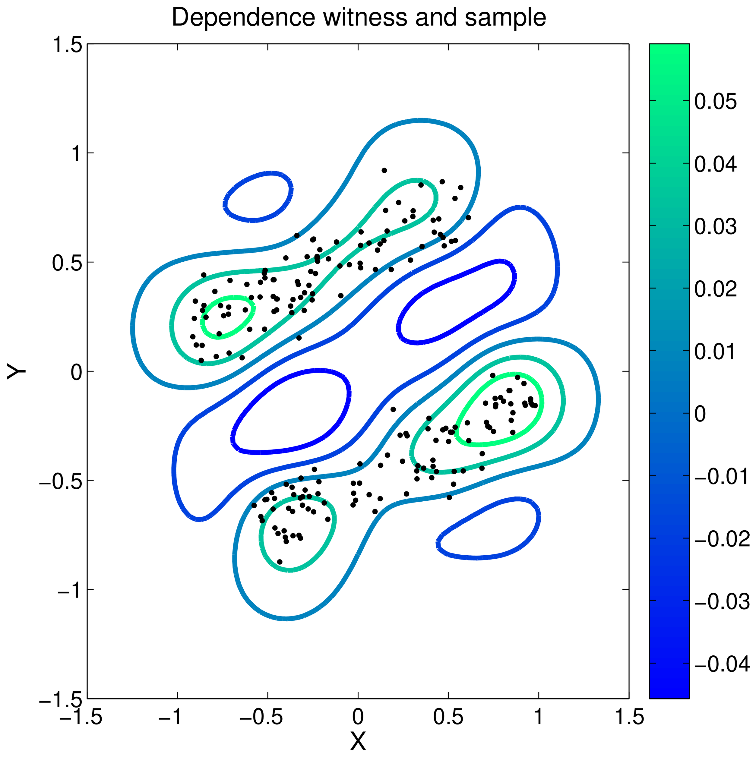 {width=60%}
We remark that a hypothesis test based on the above kernel statistic is more complicated than for the two-sample problem, since the product of the marginal distributions is in effect simulated by permuting the variables of the original sample. Further details are provided by [56].
7.4 Kernel Statistics Using a Distribution over Witness Functions
[57] define a distance between distributions as follows: let $\mathcal{H}$ be a set of functions on $\mathcal{X}$ and $r$ be a probability distribution over $\mathcal{F}$. Then the distance between two distributions $p$ and $q$ is given by
$ D(p,q) := \mathbf{E}{f \sim r(f)} \left| \mathbf{E}{x \sim p}[f(x)] - \mathbf{E}_{x \sim q}[f(x)]\right|. $
That is, we compute the average distance between $p$ and $q$ with respect to a distribution of test functions.
########## {caption="Lemma"}
Let $\mathcal{H}$ be a reproducing kernel Hilbert space, $f\in \mathcal{H}$, and assume $r(f) = r(\left|f\right|{\mathcal{H}})$ with finite $\mathbf{E}{f \sim r}[|f|\mathcal{H}]$. Then $D(p,q) = C \left|\mu[p] - \mu[q]\right|{\mathcal{H}}$ for some constant $C$ which depends only on $\mathcal{H}$ and $r$.
Proof: By definition $\mathbf{E}{p}[f(x)] = \left\langle \mu[p],f \right\rangle{\mathcal{H}}$. Using linearity of the inner product, Equation (13) equals
$ \begin{aligned} & \int \left|\left\langle \mu[p] - \mu[q],f \right\rangle_{\mathcal{H}}\right| \mathrm{d}r(f)\ = & \left|\mu[p] - \mu[q]\right|{\mathcal{H}} \int \left|\left\langle \frac{\mu[p] - \mu[q]}{\left|\mu[p] - \mu[q]\right|{\mathcal{H}}},f \right\rangle_{\mathcal{H}}\right| \mathrm{d}r(f), \end{aligned} $
where the integral is independent of $p,q$. To see this, note that for any $p,q$, $\frac{\mu[p] - \mu[q]}{\left|\mu[p] - \mu[q]\right|_{\mathcal{H}}}$ is a unit vector which can turned into, say, the first canonical basis vector by a rotation which leaves the integral invariant, bearing in mind that $r$ is rotation invariant.
7.5 Outlier Detection
An application related to the two sample problem is that of outlier detection: this is the question of whether a novel point is generated from the same distribution as a particular i.i.d. sample. In a way, this is a special case of a two sample test, where the second sample contains only one observation. Several methods essentially rely on the distance between a novel point to the sample mean in feature space to detect outliers.
For instance, [58] use a related method to deal with nonstationary time series. Likewise [59] p. 117 discuss how to detect novel observations by using the following reasoning: the probability of being an outlier is bounded both as a function of the spread of the points in feature space and the uncertainty in the empirical feature space mean (as bounded using symmetrisation and McDiarmid's tail bound).
Instead of using the sample mean and variance, [60] estimate the center and radius of a minimal enclosing sphere for the data, the advantage being that such bounds can potentially lead to more reliable tests for single observations. [61] show that the minimal enclosing sphere problem is equivalent to novelty detection by means of finding a hyperplane separating the data from the origin, at least in the case of radial basis function kernels.
8. Experiments
Section Summary: The experiments section describes tests of various MMD-based methods, along with several existing statistical tests, on both synthetic and real data drawn from database, bioinformatics, and neurobiology domains. A key implementation detail covered is the choice of kernel width for the Gaussian RBF kernel via the median pairwise distance heuristic. The first reported study examines how the tests scale with increasing dimensionality when distinguishing two Gaussians that differ either in mean or in variance, while later studies apply the same methods to data-integration tasks on microarray and neural recordings.
We conducted distribution comparisons using our MMD-based tests on datasets from three real-world domains: database applications, bioinformatics, and neurobiology. We investigated both uniform convergence approaches ($\mathrm{MMD}_b$ with the Corollary 13 threshold, and $\mathrm{MMD}^2_u$ H with the Corollary 15 threshold); the asymptotic approaches with bootstrap ($\mathrm{MMD}^2_u$ B) and moment matching to Pearson curves ($\mathrm{MMD}^2_u$ M), both described in Section 5; and the asymptotic approach using the linear time statistic ($\mathrm{MMD}^2_l$) from Section 6. We also compared against several alternatives from the literature (where applicable): the multivariate t-test, the Friedman-Rafsky Kolmogorov-Smirnov generalisation (Smir), the Friedman-Rafsky Wald-Wolfowitz generalisation (Wolf), the Biau-Györfi test (Biau), and the Hall-Tajvidi test (Hall). See Section 3.3 for details regarding these tests. Note that we do not apply the Biau-Györfi test to high-dimensional problems (since the required space partitioning is no longer possible), and that MMD is the only method applicable to structured data such as graphs.
An important issue in the practical application of the MMD-based tests is the selection of the kernel parameters. We illustrate this with a Gaussian RBF kernel, where we must choose the kernel width $\sigma$ (we use this kernel for univariate and multivariate data, but not for graphs). The empirical MMD is zero both for kernel size $\sigma=0$ (where the aggregate Gram matrix over $X$ and $Y$ is a unit matrix), and also approaches zero as $\sigma \rightarrow \infty$ (where the aggregate Gram matrix becomes uniformly constant). We set $\sigma$ to be the median distance between points in the aggregate sample, as a compromise between these two extremes: this remains a heuristic, similar to those described in [62, 63], and the optimum choice of kernel size is an ongoing area of research.
8.1 Toy Example: Two Gaussians
In our first experiment, we investigated the scaling performance of the various tests as a function of the dimensionality $d$ of the space $\mathcal{X}\subset \mathbb{R}^d$, when both $p$ and $q$ were Gaussian. We considered values of $d$ up to 2500: the performance of the MMD-based tests cannot therefore be explained in the context of density estimation (as in Section 7.1), since the associated density estimates are necessarily meaningless here. The levels for all tests were set at $\alpha=0.05$, $m=250$ samples were used, and results were averaged over $100$ repetitions. In the first case, the distributions had different means and unit variance. The percentage of times the null hypothesis was correctly rejected over a set of Euclidean distances between the distribution means (20 values logarithmically spaced from 0.05 to 50), was computed as a function of the dimensionality of the normal distributions. In case of the t-test, a ridge was added to the covariance estimate, to avoid singularity (the ratio of largest to smallest eigenvalue was ensured to be at most 2). In the second case, samples were drawn from distributions ${\cal N}(0,\mathbf{I})$ and ${\cal N}(0,\sigma^2\mathbf{I})$ with different variance. The percentage of null rejections was averaged over 20 $\sigma$ values logarithmically spaced from $10^{0.01}$ to $10$. The t-test was not compared in this case, since its output would have been irrelevant. Results are plotted in Figure 4.
In the case of Gaussians with differing means, we observe the t-test performs best in low dimensions, however its performance is severely weakened when the number of samples exceeds the number of dimensions. The performance of $MMD^2_u$ M is comparable to the t-test for low sample sizes, and outperforms all other methods for larger sample sizes. The worst performance is obtained for $MMD_u^2$ H, though $MMD_b$ also does relatively poorly: this is unsurprising given that these tests derive from distribution-free large deviation bounds, whereas the sample size is relatively small. Remarkably, $MMD^2_l$ performs quite well compared with classical tests in high dimensions.
In the case of Gaussians of differing variance, the Hall test performs best, followed closely by $MMD^2_u$. FR Wolf and (to a much greater extent) FR Smirnov both have difficulties in high dimensions, failing completely once the dimensionality becomes too great. The linear test $MMD^2_l$ again performs surprisingly well, almost matching the $MMD^2_u$ performance in the highest dimensionality. Both $MMD_u^2$H and $MMD_b$ perform poorly, the former failing completely: this is one of several illustrations we will encounter of the much greater tightness of the Corollary 13 threshold over that in Corollary 15.
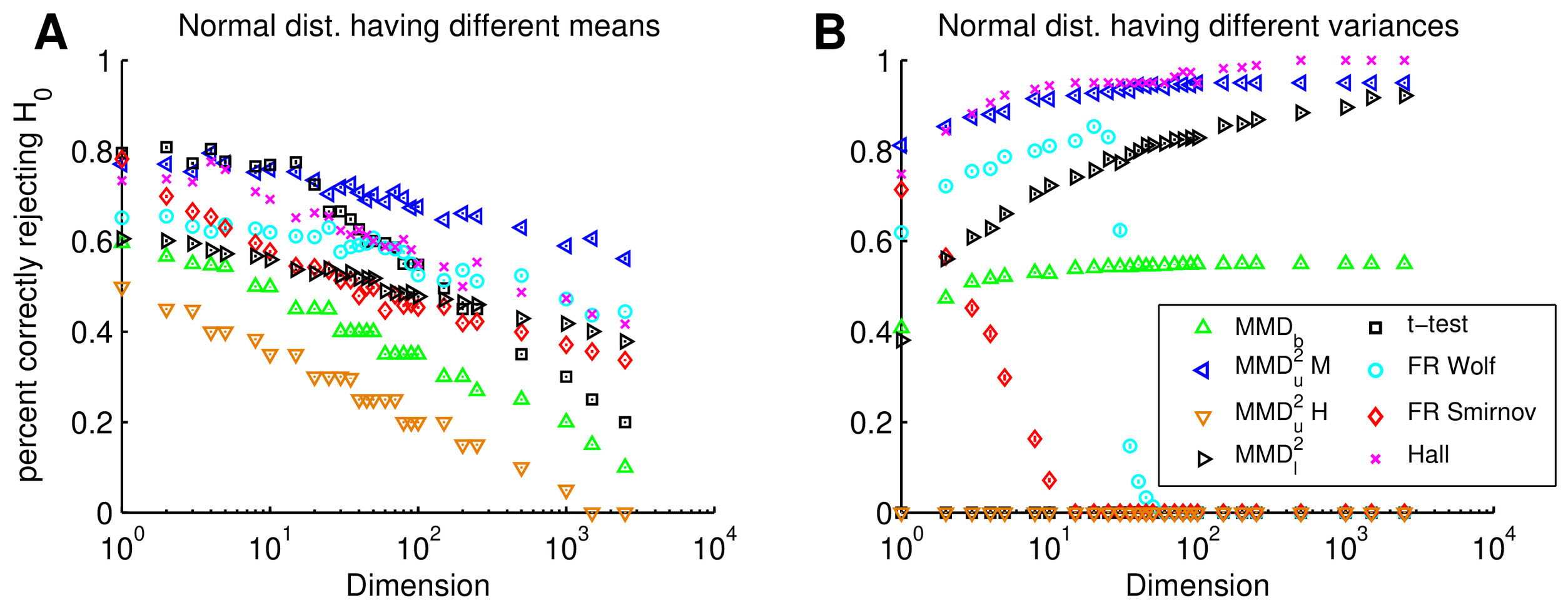
8.2 Data Integration
In our next application of MMD, we performed distribution testing for data integration: the objective being to aggregate two datasets into a single sample, with the understanding that both original samples were generated from the same distribution. Clearly, it is important to check this last condition before proceeding, or an analysis could detect patterns in the new dataset that are caused by combining the two different source distributions, and not by real-world phenomena. We chose several real-world settings to perform this task: we compared microarray data from normal and tumor tissues (Health status), microarray data from different subtypes of cancer (Subtype), and local field potential (LFP) electrode recordings from the Macaque primary visual cortex (V1) with and without spike events (Neural Data I and II, as described in more detail by [64]). In all cases, the two data sets have different statistical properties, but the detection of these differences is made difficult by the high data dimensionality (indeed, for the microarray data, density estimation is impossible given the sample size and data dimensionality, and no successful test can rely on accurate density estimates as an intermediate step).
We applied our tests to these datasets in the following fashion. Given two datasets A and B, we either chose one sample from A and the other from B (attributes = different); or both samples from either A or B (attributes = same). We then repeated this process up to 1200 times. Results are reported in Table 1. Our asymptotic tests perform better than all competitors besides Wolf: in the latter case, we have greater Type II error for one neural dataset, lower Type II error on the Health Status data (which has very high dimension and low sample size), and identical (error-free) performance on the remaining examples. We note that the Type I error of the bootstrap test on the Subtype dataset is far from its design value of $0.05$, indicating that the Pearson curves provide a better threshold estimate for these low sample sizes. For the remaining datasets, the Type I errors of the Pearson and Bootstrap approximations are close. Thus, for larger datasets, the bootstrap is to be preferred, since it costs $O(m^2)$, compared with a cost of $O(m^3)$ for Pearson (due to the cost of computing Equation (9)). Finally, the uniform convergence-based tests are too conservative, with $\mathrm{MMD}_b$ finding differences in distribution only for the data with largest sample size, and $\mathrm{MMD}^2_u$ H never finding differences.
\begin{tabular}{|l|l|r|r|r|r|r|r|r|r|r|r|} \hline
Dataset & Attr. & $\mathrm{MMD}_b$ & $\mathrm{MMD}^2_u$ H & $\mathrm{MMD}^2_u$ B& $\mathrm{MMD}^2_u$ M& t-test & Wolf & Smir & Hall \\\hline\hline
Neural Data I & Same & 100.0 & 100.0 & 96.5 & 96.5 & 100.0 &97.0 &95.0 &96.0 \\\hline
   {} & Different & 38.0 & 100.0 & \textbf{0.0} & \textbf{0.0} & 42.0 &\textbf{0.0} &10.0 &49.0 \\\hline\hline

Neural Data II & Same &100.0 & 100.0 &94.6 &95.2 &100.0 &95.0 &94.5 &96.0 \\\hline
   {} & Different &99.7 & 100.0 &3.3 &3.4$ &100.0 &\textbf{0.8} &31.8 &5.9 \\\hline\hline

Health status &Same &100.0 &100.0 &95.5 &94.4 &100.0 &94.7 &96.1 &95.6 \\\hline
  &Different &100.0 &100.0 &1.0 &\textbf{0.8} &100.0 &2.8 &44.0 &35.7 \\\hline\hline

Subtype & Same &100.0 & 100.0 &99.1 &96.4&100.0& 94.6 &97.3 &96.5 \\ \hline
   {} & Different & 100.0 &100.0 &\textbf{0.0}&\textbf{0.0} &100.0 &\textbf{0.0} &28.4 &0.2 \\\hline

\end{tabular}
8.3 Computational Cost
We next investigate the tradeoff between computational cost and performance of the various tests, with particular attention to how the quadratic time MMD tests from Section 4 and Section 5 compare with the linear time MMD-based asymptotic test from Section 6. We consider two 1-D datasets (CNUM and FOREST) and two higher-dimensional datasets (FOREST10D and NEUROII). Results are plotted in Figure 5. If cost is not a factor, then the $\mathrm{MMD}^2_u$ B shows best overall performance as a function of sample size, with a Type II error dropping to zero as fast or faster than competing approaches in three of four cases, and narrowly trailing FR Wolf in the fourth (FOREST10D). That said, for datasets CNUM, FOREST, and FOREST10D, the linear time MMD achieves results comparable to $\mathrm{MMD}^2_u$ B at a far smaller computational cost, albeit by looking at a great deal more data. In the CNUM case, however, the linear test is not able to achieve zero error even for the largest data set size. For the NEUROII data, attaining zero Type II error has about the same cost for both approaches. The difference in cost of $\mathrm{MMD}^2_u$ B and $\mathrm{MMD}_b$ is due to the bootstrapping required for the former, which produces a constant offset in cost between the two (here 150 resamplings were used).
The $t$-test also performs well in three of the four problems, and in fact represents the best cost-performance tradeoff in these three datasets (i.e. while it requires much more data than $\mathrm{MMD}^2_u$ B for a given level of performance, it costs far less to compute). The $t$-test assumes that only the difference in means is important in distinguishing the distributions, and it requires an accurate estimate of the within-sample covariance; the test fails completely on the NEUROII data. We emphasise that the Kolmogorov-Smirnov results in 1-D were obtained using the classical statistic, and not the Friedman-Rafsky statistic, hence the low computational cost. The cost of both Friedman-Rafsky statistics is therefore given by the FR Wolf cost in this case. The latter scales similarly with sample size to the quadratic time MMD tests, confirming Friedman and Rafsky's observation that obtaining the pairwise distances between sample points is the dominant cost of their tests. We also remark on the unusual behaviour of the Type II error of the FR Wolf test in the FOREST dataset, which worsens for increasing sample size.
We conclude that the approach to be recommended when testing homogeneity will depend on the data available: for small amounts of data, the best results are obtained using every observation to maximum effect, and employing the quadratic time $\mathrm{MMD}^2_u$ B test. When large volumes of data are available, a better option is to look at each point only once, which can yield greater accuracy for a given computational cost. It may also be worth doing a t-test first in this case, and only running more sophisticated non-parametric tests if the t-test accepts the null hypothesis, to verify the distributions are identical in more than just mean.
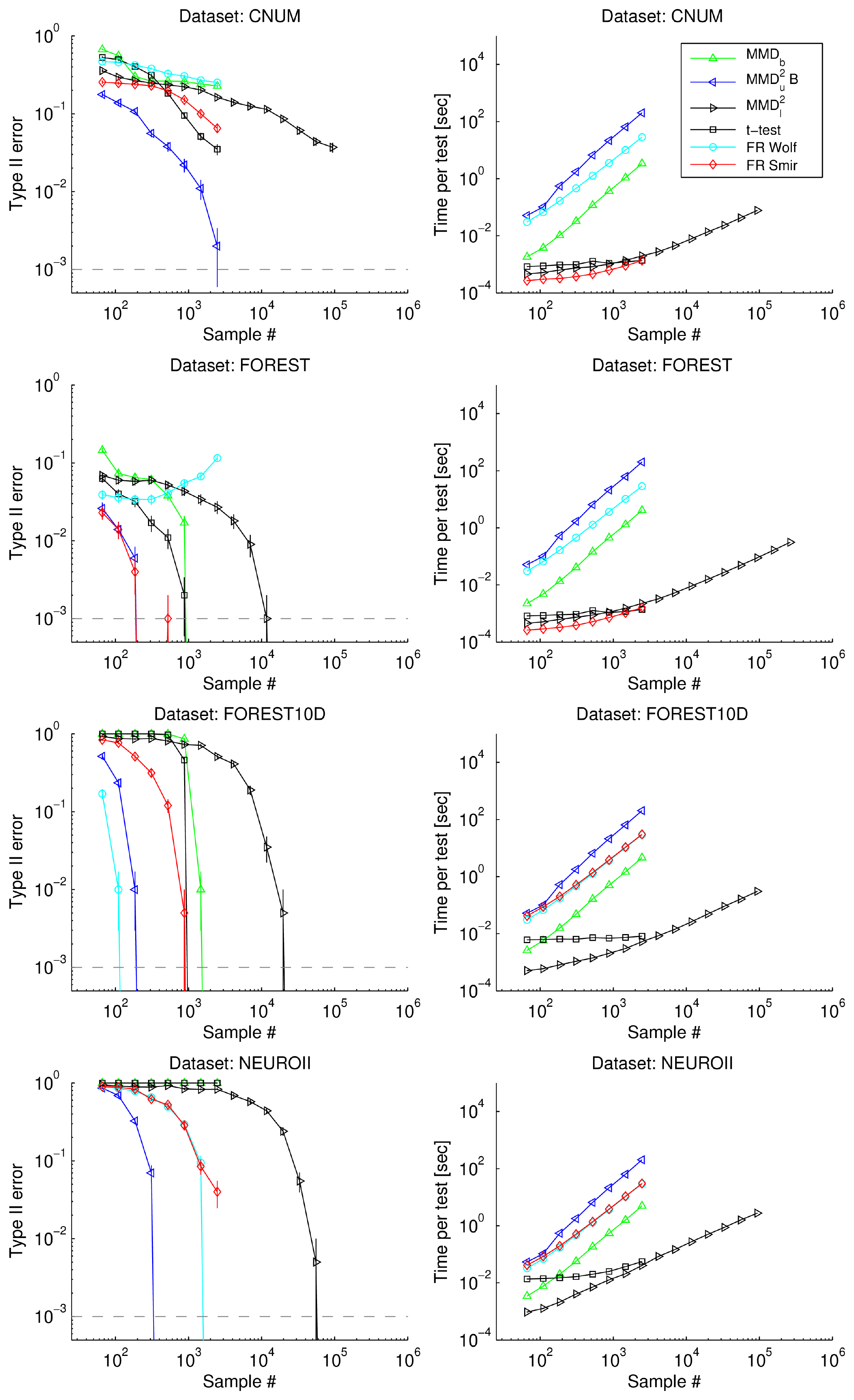
8.4 Attribute Matching
Our final series of experiments addresses automatic attribute matching. Given two databases, we want to detect corresponding attributes in the schemas of these databases, based on their data-content (as a simple example, two databases might have respective fields Wage and Salary, which are assumed to be observed via a subsampling of a particular population, and we wish to automatically determine that both Wage and Salary denote to the same underlying attribute). We use a two-sample test on pairs of attributes from two databases to find corresponding pairs.[^11] This procedure is also called table matching for tables from different databases. We performed attribute matching as follows: first, the dataset D was split into two halves A and B. Each of the $n$ attributes in A (and B, resp.) was then represented by its instances in A (resp. B). We then tested all pairs of attributes from A and from B against each other, to find the optimal assignment of attributes ${A_1,\ldots,A_n}$ from A to attributes ${B_1,\ldots,B_n}$ from $B$. We assumed that A and B contain the same number of attributes.
[^11]: Note that corresponding attributes may have different distributions in real-world databases. Hence, schema matching cannot solely rely on distribution testing. Advanced approaches to schema matching using MMD as one key statistical test are a topic of current research.
As a naive approach, one could assume that any possible pair of attributes might correspond, and thus that every attribute of $A$ needs to be tested against all the attributes of $B$ to find the optimal match. We report results for this naive approach, aggregated over all pairs of possible attribute matches, in Table 2. We used three datasets: the census income dataset from the UCI KDD archive (CNUM), the protein homology dataset from the 2004 KDD Cup (BIO) ([65]), and the forest dataset from the UCI ML archive ([66]). For the final dataset, we performed univariate matching of attributes (FOREST) and multivariate matching of tables (FOREST10D) from two different databases, where each table represents one type of forest. Both our asymptotic $\mathrm{MMD}^2_u$-based tests perform as well as or better than the alternatives, notably for CNUM, where the advantage of $\mathrm{MMD}^2_u$ is large. Unlike in Table 1, the next best alternatives are not consistently the same across all data: e.g. in BIO they are Wolf or Hall, whereas in FOREST they are Smir, Biau, or the t-test. Thus, $\mathrm{MMD}^2_u$ appears to perform more consistently across the multiple datasets. The Friedman-Rafsky tests do not always return a Type I error close to the design parameter: for instance, Wolf has a Type I error of 9.7% on the BIO dataset (on these data, $\mathrm{MMD}^2_u$ has the joint best Type II error without compromising the designed Type I performance). Finally, $\mathrm{MMD}_b$ performs much better than in Table 1, although surprisingly it fails to reliably detect differences in FOREST10D. The results of $\mathrm{MMD}^2_u$ H are also improved, although it remains among the worst performing methods.
A more principled approach to attribute matching is also possible. Assume that $\phi(A) = (\phi_1(A_1), \phi_2(A_2), ..., \phi_n(A_n))$: in other words, the kernel decomposes into kernels on the individual attributes of A (and also decomposes this way on the attributes of B). In this case, $MMD^2$ can be written $\sum_{i=1}^{n} |\mu_i(A_i) - \mu_i(B_i)|^2,$ where we sum over the MMD terms on each of the attributes. Our goal of optimally assigning attributes from $B$ to attributes of $A$ via MMD is equivalent to finding the optimal permutation $\pi$ of attributes of $B$ that minimizes $\sum_{i=1}^{n} |\mu_i(A_i) - \mu_i(B_{\pi(i)})|^2.$ If we define $C_{ij} = |\mu_i(A_i) - \mu_i(B_j)|^2$, then this is the same as minimizing the sum over $C_{i, \pi(i)}$. This is the linear assignment problem, which costs $O(n^3)$ time using the Hungarian method ([67]).
While this may appear to be a crude heuristic, it nonetheless defines a semi-metric on the sample spaces $X$ and $Y$ and the corresponding distributions $p$ and $q$. This follows from the fact that matching distances are proper metrics if the matching cost functions are metrics. We formalize this as follows:
########## {caption="Theorem"}
Let $p, q$ be distributions on $\mathbb{R}^d$ and denote by $p_i, q_i$ the marginal distributions on the $i$-th variable. Moreover, denote by $\Pi$ the symmetric group on $\left{1, \ldots, d\right}$. The following distance, obtained by optimal coordinate matching, is a semi-metric.
$ \Delta[\mathcal{F}, p, q] := \min_{\pi \in \Pi} \sum_{i=1}^d \mathrm{MMD}[\mathcal{F}, p_i, q_{\pi(i)}] $
Proof: Clearly $\Delta[\mathcal{F}, p, q]$ is nonnegative, since all of its summands are. Next we show the triangle inequality. Denote by $r$ a third distribution on $\mathbb{R}^d$ and let $\pi_{p,q}, \pi_{q,r}$ and $\pi_{p,r}$ be the distance minimizing permutations between $p, q$ and $r$ respectively. It then follows that
$ \begin{aligned} \Delta[\mathcal{F}, p, q] + \Delta[\mathcal{F}, q, r] & = \sum_{i=1}^d \mathrm{MMD}[\mathcal{F}, p_i, q_{\pi_{p,q}(i)}] + \sum_{i=1}^d \mathrm{MMD}[\mathcal{F}, q_i, r_{\pi_{q,r}(i)}] \ & \geq \sum_{i=1}^d \mathrm{MMD}[\mathcal{F}, p_i, r_{\pi_{p,q} \circ \pi_{q,r}}] \geq \Delta[\mathcal{F}, p, r]. \end{aligned} $
Here the first inequality follows from the triangle inequality on $\mathrm{MMD}$, that is
$ \mathrm{MMD}[\mathcal{F}, p_i, q_{\pi_{p,q}(i)}] + \mathrm{MMD}[\mathcal{F}, q_{\pi_{p,q}(i)}, r_{\pi_{p,q} \circ \pi_{q,r}}] \geq \mathrm{MMD}[\mathcal{F}, p_i, r_{\pi_{p,q} \circ \pi_{q,r}}]. $
The second inequality is a result of minimization over $\pi$.
\begin{tabular}{|l|l|r|r|r|r|r|r|r|r|r|} \hline

Dataset & Attr. & $\mathrm{MMD}_b$ & $\mathrm{MMD}^2_u$ H & $\mathrm{MMD}^2_u$ B& $\mathrm{MMD}^2_u$ M&t-test &Wolf & Smir & Hall & Biau\\\hline\hline
BIO& Same &100.0 & 100.0 &93.8 &94.8&95.2 &90.3 &95.8 &95.3 &99.3 \\\hline
   {} & Different &20.0 & 52.6 &\textbf{17.2}&17.6 &36.2 &\textbf{17.2} &18.6 &17.9 &42.1 \\\hline\hline

FOREST & Same &100.0& 100.0 &96.4 &96.0 &97.4 &94.6 &99.8 &95.5 &100.0 \\\hline
   {} & Different& 3.9 & 11.0 &\textbf{0.0} &\textbf{0.0} &0.2 &3.8 &\textbf{0.0} &50.1 &\textbf{0.0} \\\hline\hline

CNUM & Same &100.0& 100.0 & 94.5 & 93.8 &94.0 &98.4 &97.5 &91.2 &98.5 \\\hline
   {} & Different &14.9 & 52.7 & 2.7& \textbf{2.5}&19.17 &22.5 &11.6 &79.1 &50.5 \\\hline\hline

FOREST10D & Same &100.0 & 100.0 &94.0 &94.0 &100.0 &93.5 &96.5 & 97.0 &100.0 \\\hline
   {} & Different &86.6 &100.0 &\textbf{0.0} &\textbf{0.0} &\textbf{0.0} &\textbf{0.0} &1.0 & 72.0 & 100.0 \\\hline

 \end{tabular}
We tested this 'Hungarian approach' to attribute matching via $\mathrm{MMD}^2_u$ B on three univariate datasets (BIO, CNUM, FOREST) and for table matching on a fourth (FOREST10D). To study $\mathrm{MMD}^2_u$ B on structured data, we obtained two datasets of protein graphs (PROTEINS and ENZYMES) and used the graph kernel for proteins from [68] for table matching via the Hungarian method (the other tests were not applicable to this graph data). The challenge here is to match tables representing one functional class of proteins (or enzymes) from dataset A to the corresponding tables (functional classes) in B. Results are shown in Table 3. Besides on the BIO and CNUM datasets, $\mathrm{MMD}^2_u$ B made no errors.
: Table 3: Hungarian Method for attribute matching via $\mathrm{MMD}^2_u$ B on univariate (BIO, CNUM, FOREST), multivariate (FOREST10D), and structured data (ENZYMES, PROTEINS) ($\alpha=0.05$; '% correct matches' is the percentage of the correct attribute matches detected over all repetitions).
| Dataset | Data type | No. attributes | Sample size | Repetitions | % correct matches |
|---|---|---|---|---|---|
| BIO | univariate | 6 | 377 | 100 | 90.0 |
| CNUM | univariate | 13 | 386 | 100 | 99.8 |
| FOREST | univariate | 10 | 538 | 100 | 100.0 |
| FOREST10D | multivariate | 2 | 1000 | 100 | 100.0 |
| ENZYME | structured | 6 | 50 | 50 | 100.0 |
| PROTEINS | structured | 2 | 200 | 50 | 100.0 |
9. Conclusion
Section Summary: The authors developed three straightforward statistical tests based on maximum mean discrepancy to determine whether two sets of data samples come from the same underlying distribution, without needing to estimate densities as an intermediate step. Two of the tests give exact error control that holds regardless of the data distribution or sample size, while all three run efficiently in quadratic or even linear time and cover several classical comparison methods. The section also notes connections to related kernel techniques and classical distances, pointing to opportunities for extending the framework.
We have established three simple multivariate tests for comparing two distributions $p$ and $q$, based on samples of size $m$ and $n$ from these respective distributions. Our test statistic is the maximum mean discrepancy (MMD), defined as the maximum deviation in the expectation of a function evaluated on each of the random variables, taken over a sufficiently rich function class: in our case, a universal reproducing kernel Hilbert space (RKHS). Equivalently, the statistic can be written as the norm of the difference between distribution feature means in the RKHS. We do not require density estimates as an intermediate step. Two of our tests provide Type I error bounds that are exact and distribution-free for finite sample sizes. We also give a third test based on quantiles of the asymptotic distribution of the associated test statistic. All three tests can be computed in $O((m+n)^2)$ time, however when sufficient data are available, a linear time statistic can be used, which employs more data to get better results at smaller computational cost. In addition, a number of metrics on distributions (Kolmogorov-Smirnov, Earth Mover's, $L_2$ distance between Parzen window density estimates), as well as certain kernel similarity measures on distributions, are included within our framework.
While our result establishes that statistical tests based on the MMD are consistent for universal kernels on compact domains, we draw attention to the recent introduction of characteristic kernels by [69], these being kernels for which the mean map is injective. Fukumizu et al. establish that Gaussian and Laplace kernels are characteristic on $\mathbb{R}^d$, and thus the MMD is a consistent test for this domain. [70] further explore the properties of characteristic kernels, providing a simple condition to determine whether convolution kernels are characteristic, and describing characteristic kernels which are not universal on compact domains. We also note (following Section 7.2) that the MMD for RKHSs is associated with a particular kernel between probability distributions. [47] describe several further such kernels, which induce corresponding distances between feature space distribution mappings: these may in turn lead to new and powerful two-sample tests.
Two recent studies have shown that additional divergence measures between distributions can be obtained empirically through optimization in a reproducing kernel Hilbert space. [12] build on the work of [2], considering a homogeneity statistic arising from the kernel Fisher discriminant, rather than the difference of RKHS means; and [71] obtain a KL divergence estimate by approximating the ratio of densities (or its log) with a function in an RKHS. By design, both these kernel-based statistics prioritise different features of $p$ and $q$ when measuring the divergence between them, and the resulting effects on distinguishability of distributions are therefore of interest.
Finally, we have seen in Section 2 that several classical metrics on probability distributions can be written as maximum mean discrepancies with function classes that are not Hilbert spaces, but rather Banach, metric, or semi-metric spaces. It would be of particular interest to establish under what conditions one could write these discrepancies in terms of norms of differences of mean elements. In particular, [72] consider Banach spaces endowed with a semi-inner product, for which a General Riesz Representation exists for elements in the dual.
Appendix
Section Summary: The appendix establishes finite-sample guarantees for a statistical test based on maximum mean discrepancy by deriving concentration bounds on the deviation between the true MMD and its empirical estimate. It first recalls McDiarmid’s inequality and Rademacher averages, then applies them to show that the deviation probability decays exponentially in the sample sizes whether the two distributions are identical or different. A specialized version of the same argument is given for the equal-sample, equal-distribution case needed by the hypothesis test.
A. Large Deviation Bounds for Tests with Finite Sample Guarantees
A.1 Preliminary Definitions and Theorems
We need the following theorem, due to [27].
########## {caption="Theorem: McDiarmid's inequality"}
Let $f,:,\mathcal{X}^{m}\rightarrow \mathbb{R}$ be a function such that for all $i\in{1,\ldots,m}$, there exist $c_{i}<\infty$ for which
$ \sup_{X\in\mathcal{X}^{m},\tilde{x}\in\mathcal{X}}|f(x_{1},\ldots x_{m})-f(x_{1},\ldots x_{i-1},\tilde{x},x_{i+1},\ldots,x_{m})|\le c_{i}. $
Then for all probability measures $p$ and every $\epsilon>0$,
$ p_{\mathsf{x}^{m}}\left(f(\mathbf{x})-\mathbf{E}{\mathsf{x}^{m}}(f(\mathbf{x}))>t\right)<\exp\left(-\frac{2\epsilon^{2}}{\sum{i=1}^{m}c_{i}^{2}}\right). $
We also define the Rademacher average of the function class $\mathcal{F}$ with respect to the $m$-sample $X$.
########## {caption="Definition 19: Rademacher average of $\mathcal{F}$ on $X
quot;}Let $\mathcal{F}$ be the unit ball in a universal RKHS on the compact domain $\mathcal{X}$, with kernel bounded according to $0\le k(x,y)\le K$. Let $X$ be an i.i.d. sample of size $m$ drawn according to a probability measure $p$ on $\mathcal{X}$, and let $\sigma_{i}$ be i.i.d and take values in ${-1,1}$ with equal probability. We define the Rademacher average
$ \begin{aligned} R_{m}(\mathcal{F},X) & := \mathbf{E}{\sigma}\sup{f\in \mathcal{F}}\left|\frac{1}{m}\sum_{i=1}^{m}\sigma_{i}f(x_{i})\right|\ & \le \left(K/m\right)^{1/2}, \end{aligned} $
where the upper bound is due to [73] Lemma 22. Similarly, we define
$ R_{m}(\mathcal{F},p) := \mathbf{E}{p,\sigma}\sup{f\in \mathcal{F}}\left|\frac{1}{m}\sum_{i=1}^{m}\sigma_{i}f(x_{i})\right|. $
A.2 Bound when $p$ and $q$ May Differ
We want to show that the absolute difference between $\mathrm{MMD}(\mathcal{F},p,q)$ and $\mathrm{MMD}_b(\mathcal{F},X,Y)$ is close to its expected value, independent of the distributions $p$ and $q$. To this end, we prove three intermediate results, which we then combine. The first result we need is an upper bound on the absolute difference between $\mathrm{MMD}(\mathcal{F},p,q)$ and $\mathrm{MMD}_b(\mathcal{F},X,Y)$. We have
$ \begin{aligned} & \left| \mathrm{MMD}(\mathcal{F},p,q)-\mathrm{MMD}b(\mathcal{F},X,Y)\right| \nonumber\ & = \left|\sup{f\in \mathcal{F}}\left(\mathbf{E}{p}(f)-\mathbf{E}{q}(f)\right)-\sup_{f\in \mathcal{F}}\left(\frac{1}{m}\sum_{i=1}^{m}f(x_{i})-\frac{1}{n}\sum_{i=1}^{n}f(y_{i})\right)\right| \nonumber\ & \le \underset{\Delta(p,q,X,Y)}{\underbrace{\sup_{f\in \mathcal{F}}\left| \mathbf{E}{p}(f)-\mathbf{E}{q}(f)-\frac{1}{m}\sum_{i=1}^{m}f(x_{i})+\frac{1}{n}\sum_{i=1}^{n}f(y_{i})\right|}}. \end{aligned} $
Second, we provide an upper bound on the difference between $\Delta(p,q,X,Y)$ and its expectation. Changing either of $x_{i}$ or $y_{i}$ in $\Delta(p,q,X,Y)$ results in changes in magnitude of at most $2K^{1/2}/m$ or $2K^{1/2}/n$, respectively. We can then apply McDiarmid's theorem, given a denominator in the exponent of
$ m\left(2K^{1/2}/m\right)^{2}+n\left(2K^{1/2}/n\right)^{2}=4K\left(\frac{1}{m}+\frac{1}{n}\right)=4K\frac{m+n}{mn}, $
to obtain
$ \Pr\left(\Delta(p,q,X,Y)-\mathbf{E}_{X,Y}\left[\Delta(p,q,X,Y)\right]>\epsilon\right)\le\exp\left(-\frac{\epsilon^{2}mn}{2K(m+n)}\right). $
For our final result, we exploit symmetrisation, following e.g. [74], p. 108, to upper bound the expectation of $\Delta(p,q,X,Y)$. Denoting by $X'$ an i.i.d sample of size $m$ drawn independently of $X$ (and likewise for $Y'$), we have
$ \begin{aligned} & \mathbf{E}{X,Y}\left[\Delta(p,q,X,Y)\right]\nonumber\ & = \mathbf{E}{X,Y}\sup_{f\in \mathcal{F}}\left| \mathbf{E}{p}(f)-\frac{1}{m}\sum{i=1}^{m}f(x_{i})-\mathbf{E}{q}(f)+\frac{1}{n}\sum{i=1}^{n}f(y_{j})\right|\nonumber\ & = \mathbf{E}{X,Y}\sup{f\in \mathcal{F}}\left| \mathbf{E}{X'}\left(\frac{1}{m}\sum{i=1}^{m}f(x_{i}')\right)-\frac{1}{m}\sum_{i=1}^{m}f(x_{i})-\mathbf{E}{Y'}\left(\frac{1}{n}\sum{i=1}^{n}f(y_{j}')\right)+\frac{1}{n}\sum_{i=1}^{n}f(y_{j})\right|\nonumber\ & \underset{(a)}{\le} \mathbf{E}{X,Y,X',Y'}\sup{f\in \mathcal{F}}\left|\frac{1}{m}\sum_{i=1}^{m}f(x_{i}')-\frac{1}{m}\sum_{i=1}^{m}f(x_{i})-\frac{1}{n}\sum_{i=1}^{n}f(y_{j}')+\frac{1}{n}\sum_{i=1}^{n}f(y_{j})\right|\nonumber\ & = \mathbf{E}{X,Y,X',Y',\sigma,\sigma'}\sup{f\in \mathcal{F}}\left|\frac{1}{m}\sum_{i=1}^{m}\sigma_{i}\left(f(x_{i}')-f(x_{i})\right)+\frac{1}{n}\sum_{i=1}^{n}\sigma_{i}'\left(f(y_{j}')-f(y_{j})\right)\right|\nonumber\ & \underset{(b)}{\le} \mathbf{E}{X,X'\sigma}\sup{f\in \mathcal{F}}\left|\frac{1}{m}\sum_{i=1}^{m}\sigma_{i}\left(f(x_{i}')-f(x_{i})\right)\right|+\mathbf{E}{Y,Y'\sigma}\sup{f\in \mathcal{F}}\left|\frac{1}{n}\sum_{i=1}^{n}\sigma_{i}\left(f(y_{j}')-f(y_{j})\right)\right|\nonumber\ & \underset{(c)}{\le} 2\left[R_{m}(\mathcal{F},p)+R_{n}(\mathcal{F},q)\right].\nonumber\ & \underset{(d)}{\le} 2\left[(K/m)^{1/2} + (K/n)^{1/2} \right], \end{aligned} $
where (a) uses Jensen's inequality, (b) uses the triangle inequality, (c) substitutes Definition 19 (the Rademacher average), and (d) bounds the Rademacher averages, also via Definition 19.
Having established our preliminary results, we proceed to the proof of Theorem 11.
Theorem 11: Combining equations (15) and (16), gives
$ \Pr\left(\Delta(p,q,X,Y)- 2\left[(K/m)^{1/2} + (K/n)^{1/2} \right] >\epsilon\right)\le\exp\left(-\frac{\epsilon^{2}mn}{2K(m+n)}\right). $
Substituting equation (14) yields the result.
A.3 Bound when $p=q$ and $m=n$
In this section, we derive the Theorem 12 result, namely the large deviation bound on the MMD when $p=q$ and $m=n$. Note also that we consider only positive deviations of $\mathrm{MMD}_b(\mathcal{F},X,Y)$ from $\mathrm{MMD}(\mathcal{F},p,q)$, since negative deviations are irrelevant to our hypothesis test. The proof follows the same three steps as in the previous section. The first step in Equation (14) becomes
$ \begin{aligned} \mathrm{MMD}b(\mathcal{F},X,Y)-\mathrm{MMD}(\mathcal{F},p,q) & = \mathrm{MMD}b(\mathcal{F},X,X')-0\nonumber \ & = \sup{f\in \mathcal{F}}\left(\frac{1}{m}\sum{i=1}^{m}\left(f(x_{i})-f(x_{i}')\right)\right). \end{aligned} $
The McDiarmid bound on the difference between Equation (17) and its expectation is now a function of $2m$ observations in Equation (17), and has a denominator in the exponent of $2m\left(2K^{1/2}/m\right)^{2}=8K/m$. We use a different strategy in obtaining an upper bound on the expected Equation (17), however: this is now
$ \begin{aligned} & \mathbf{E}{X,X'}\left[\sup{f\in \mathcal{F}}\frac{1}{m}\sum_{i=1}^{m}\left(f(x_{i})-f(x_{i}')\right)\right] \nonumber\ & = \frac{1}{m}\mathbf{E}{X,X'}\left\Vert \sum{i=1}^{m}\left(\phi(x_{i})-\phi(x_{i}')\right)\right\Vert \nonumber \ & = \frac{1}{m}\mathbf{E}{X,X'}\left[\sum{i=1}^{m}\sum_{j=1}^{m}\left(k(x_{i},x_{j})+k(x_{i}',x_{j}')-k(x_{i},x'{j})-k(x{i}',x_{j})\right)\right]^{\frac{1}{2}}\nonumber \ & \le \frac{1}{m}\left[2m \mathbf{E}{x}k(x,x)+2m(m-1)\mathbf{E}{x,x'}k(x,x')-2m^{2}\mathbf{E}{x,x'}k(x,x')\right]^{\frac{1}{2}}\nonumber\ & = \left[\frac{2}{m}\mathbf{E}{x,x'}\left(k(x,x)-k(x,x')\right)\right]^{\frac{1}{2}}\quad\text{(a)}\ & \le \left(2K/m\right)^{1/2}.\quad\text{(b)} \end{aligned} $
We remark that both Equation (18a) and (18b) bound the amount by which our biased estimate of the population MMD exceeds zero under $\mathcal{H}{0}$. Combining the three results, we find that under $\mathcal{H}{0}$,
$ \begin{aligned} p_{X}\left(\mathrm{MMD}b(\mathcal{F},X,X')-\left[\frac{2}{m}\mathbf{E}{x,x'}\left(k(x,x)-k(x,x')\right)\right]^{\frac{1}{2}}>\epsilon\right) & < \exp\left(\frac{-\epsilon^{2}m}{4K}\right)\quad\mathrm{and}\ p_{X}\left(\mathrm{MMD}_b(\mathcal{F},X,X')-\left(2K/m\right)^{1/2}>\epsilon\right) & < \exp\left(\frac{-\epsilon^{2}m}{4K}\right). \end{aligned} $
B. Proofs for Asymptotic Tests
We derive results needed in the asymptotic test of Section 5. Appendix B.1 describes the distribution of the empirical MMD under $\mathcal{H}_0$ (both distributions identical). Appendix B.2 contains derivations of the second and third moments of the empirical MMD, also under $\mathcal{H}_0$.
B.1 Convergence of the Empirical MMD under $\mathcal{H}_0$
We describe the distribution of the unbiased estimator $\mathrm{MMD}{u}^{2}[\mathcal{F},X,Y]$ under the null hypothesis. In this circumstance, we denote it by $\mathrm{MMD}{u}^{2}[\mathcal{F},X,X']$, to emphasise that the second sample $X'$ is drawn independently from the same distribution as $X$. We thus obtain the U-statistic
$ \begin{aligned} \mathrm{MMD}{u}^{2}[\mathcal{F},X,X'] & = \frac{1}{m(m-1)}\sum{i\neq j}k(x_{i},x_{j})+k(x'{i},x'{j})-k(x_{i},x'{j})-k(x{j},x'{i})\quad\text{(a)}\ & = \frac{1}{m(m-1)}\sum{i\neq j}h(z_{i},z_{j}),\quad\text{(b)} \end{aligned} $
where $z_{i}=(x_{i},x_{i}')$. Under the null hypothesis, this U-statistic is degenerate, meaning
$ \begin{aligned} \mathbf{E}{z{j}}h(z_{i},z_{j}) & = \mathbf{E}{x{j}}k(x_{i},x_{j})+\mathbf{E}{x{j}'}k(x'{i},x'{j})-\mathbf{E}{x{j}'}k(x_{i},x_{j}')-\mathbf{E}{x{j}}k(x_{j},x_{i}')\ & = 0. \end{aligned} $
The following theorem from [11], Section 5.5.2 then applies.
########## {caption="Theorem"}
Assume $\mathrm{MMD}{u}^{2}[\mathcal{F},X,X']$ is as defined in Equation (19b), with $\mathbf{E}{z'}h(z,z')=0$, and furthermore assume $0 < \mathbf{E}{z,z'}h^{2}(z,z') < \infty$. Then $\mathrm{MMD}{u}^{2}[\mathcal{F},X,X']$ converges in distribution according to
$ m \mathrm{MMD}{u}^{2}[\mathcal{F},X,X']\overset{D}{\rightarrow}\sum{l=1}^{\infty}\gamma_{l}\left(\chi_{1l}^{2}-1\right), $
where $\chi_{1l}^{2}$ are independent chi squared random variables of degree one, and $\gamma_{l}$ are the solutions to the eigenvalue equation
$ \gamma_{l}\psi_{l}(u)=\int h(u,v)\psi_{l}(v)d\Pr_{v}. $
While this result is adequate for our purposes (since we do not explicitly use the quantities $\gamma_{l}$ in our subsequent reasoning), it does not make clear the dependence of the null distribution on the kernel choice. For this reason, we provide an alternative expression based on the reasoning of [25], Appendix, bearing in mind the following changes:
- we do not need to deal with the bias terms $S_{1j}$ seen by [25], Appendix that vanish for large sample sizes, since our statistic is unbiased (although these bias terms drop faster than the variance);
- we require greater generality, since we deal with distributions on compact metric spaces, and not densities on $\mathbb{R}^{d}$; correspondingly, our kernels are not necessarily inner products in $L_{2}$ between probability density functions (although this is a special case).
Our first step is to express the kernel $h(z_{i},z_{j})$ of the U-statistic in terms of an RKHS kernel $\tilde{k}(x_{i},x_{j})$ between feature space mappings from which the mean has been subtracted,
$ \begin{aligned} \tilde{k}(x_{i},x_{j}) & := \left\langle \phi(x_{i})-\mu[p],\phi(x_{j})-\mu[p]\right\rangle \ & = k(x_{i},x_{j})-\mathbf{E}{x}k(x{i},x)-\mathbf{E}{x}k(x,x{j})+\mathbf{E}_{x,x'}k(x,x'). \end{aligned} $
The centering terms cancel (the distance between the two points is unaffected by an identical global shift in both the points), meaning
$ h(z_{i},z_{j})=\tilde{k}(x_{i},x_{j})+\tilde{k}(y_{i},y_{j})-\tilde{k}(x_{i},y_{j})-\tilde{k}(x_{j},y_{i}). $
Next, we write the kernel $\tilde{k}(x_{i},x_{j})$ in terms of eigenfunctions $\psi_{i}(x)$ with respect to the probability measure $\Pr_{x}$,
$ \tilde{k}(x,x')=\sum_{l=1}^{\infty}\lambda_{l}\psi_{l}(x)\psi_{l}(x'), $
where
$ \int_{\mathcal{X}}\tilde{k}(x,x')\psi_{i}(x)d\Pr_{x}(x)=\lambda_{i}\psi_{i}(x') $
and
$ \int_{\mathcal{X}}\psi_{i}(x)\psi_{j}(x)d\Pr_{x}(x)=\delta_{ij}. $
Since
$ \begin{aligned} \mathbf{E}{x}\tilde{k}(x,v) & = \mathbf{E}{x}k(x,v)-\mathbf{E}{x,x'}k(x,x')-\mathbf{E}{x}k(x,v)+\mathbf{E}_{x,x'}k(x,x')\ & = 0, \end{aligned} $
then when $\lambda_{i}\neq0,$ we have that
$ \begin{aligned} \lambda_{i}\mathbf{E}{x'}\psi{i}(x') & = \int_{\mathcal{X}}\mathbf{E}{x'}\tilde{k}(x,x')\psi{i}(x)d\Pr_{x}(x)\ & = 0, \end{aligned} $
and hence
$ \mathbf{E}{x}\psi{i}(x)=0. $
We now use these results to transform the expression in Equation (19a). First,
$ \begin{aligned} \frac{1}{m}\sum_{i\neq j}\tilde{k}(x_{i},x_{j}) & = \frac{1}{m}\sum_{i\neq j}\sum_{l=1}^{\infty}\lambda_{l}\psi_{l}(x_{i})\psi_{l}(x_{j})\ & = \frac{1}{m}\sum_{l=1}^{\infty}\lambda_{l}\left(\left(\sum_{i}\psi_{l}(x_{i})\right)^{2}-\sum_{i}\psi_{l}^{2}(x_{i})\right)\ & \underset{D}{\rightarrow} \sum_{l=1}^{\infty}\lambda_{l}(y_{l}^{2}-1), \end{aligned} $
where $y_{l}\sim\mathcal{N}(0,1)$ are i.i.d., and the final relation denotes convergence in distribution, using Equation (20) and (21), following [11], Section 5.5.2. Likewise
$ \begin{aligned} \frac{1}{m}\sum_{i\neq j}\tilde{k}(x_{i}',x_{j}') & \underset{D}{\rightarrow} \sum_{l=1}^{\infty}\lambda_{l}(z_{l}^{2}-1), \end{aligned} $
where $z_{l}\sim\mathcal{N}(0,1)$, and
$ \begin{aligned} \frac{1}{m(m-1)}\sum_{i\neq j}\left(\tilde{k}(x_{i},y_{j})+\tilde{k}(x_{j},y_{i})\right) & \underset{D}{\rightarrow} 2\sum_{l=1}^{\infty}\lambda_{l}y_{l}z_{l}. \end{aligned} $
Combining these results, we get
$ \begin{aligned} m\mathrm{MMD}^2_u(\mathcal{F},X,X') & \underset{D}{\rightarrow} \sum_{l=1}^{\infty}\lambda_{l}\left(y_{l}^{2}+z_{l}^{2}-2-2y_{l}z_{l}\right)\ & = \sum_{l=1}^{\infty}\lambda_{l}\left[(y_{l}-z_{l})^{2}-2\right]. \end{aligned} $
Note that $y_{l}-z_{l}$, being the difference of two independent Gaussian variables, has a normal distribution with mean zero and variance $2$. This is therefore a quadratic form in a Gaussian random variable minus an offset $2\sum_{l=1}^{\infty}\lambda_{l}$.
B.2 Moments of the Empirical MMD Under $\mathcal{H}_0$
In this section, we compute the moments of the U-statistic in Section 5, under the null hypothesis conditions
$ \begin{aligned} \mathbf{E}_{z,z'}h(z,z')& =0, \quad\text{(a)} \end{aligned} $
and, importantly,
$ \begin{aligned} \mathbf{E}_{z'}h(z,z')&=0. \quad\text{(b)} \end{aligned} $
Note that the latter implies the former.
Variance/2nd moment: This was derived by [75], p. 299, and is also described by [11], Lemma A p. 183. Applying these results,
$ \begin{aligned} & \mathbf{E}\left(\left[\mathrm{MMD}u^2\right]^2\right) \ & = \left(\frac{2}{n(n-1)}\right)^{2}\left[\frac{n(n-1)}{2}(n-2)(2)\mathbf{E}{z}\left[(\mathbf{E}{z'}h(z,z'))^{2}\right]+\frac{n(n-1)}{2}\mathbf{E}{z,z'}\left[h^{2}(z,z')\right]\right] \ & = \frac{2(n-2)}{n(n-1)}\mathbf{E}{z}\left[(\mathbf{E}{z'}h(z,z'))^{2}\right]+\frac{2}{n(n-1)}\mathbf{E}{z,z'}\left[h^{2}(z,z')\right]\ & = \frac{2}{n(n-1)}\mathbf{E}{z,z'}\left[h^{2}(z,z')\right], \end{aligned} $
where the first term in the penultimate line is zero due to (22b). Note that variance and 2nd moment are the same under the zero mean assumption.
3rd moment: We consider the terms that appear in the expansion of $\mathbf{E}\left(\left[\mathrm{MMD}_u^2\right]^3\right)$. These are all of the form
$ \left(\frac{2}{n(n-1)}\right)^{3}\mathbf{E}(h_{ab}h_{cd}h_{ef}), $
where we shorten $h_{ab}=h(z_{a},z_{b})$, and we know $z_{a}$ and $z_{b}$ are always independent. Most of the terms vanish due to (22a) and (22b). The first terms that remain take the form
$ \left(\frac{2}{n(n-1)}\right)^{3}\mathbf{E}(h_{ab}h_{bc}h_{ca}), $
and there are
$ \frac{n(n-1)}{2}(n-2)(2) $
of them, which gives us the expression
$ \begin{aligned} & \left(\frac{2}{n(n-1)}\right)^{3}\frac{n(n-1)}{2}(n-2)(2)\mathbf{E}{z,z'}\left[h(z,z')\mathbf{E}{z''}\left(h(z,z'')h(z',z'')\right)\right]\nonumber \ & = \frac{8(n-2)}{n^{2}(n-1)^{2}}\mathbf{E}{z,z'}\left[h(z,z')\mathbf{E}{z''}\left(h(z,z'')h(z',z'')\right)\right]. \end{aligned} $
Note the scaling $\frac{8(n-2)}{n^{2}(n-1)^{2}}\sim\frac{1}{n^{3}}$. The remaining non-zero terms, for which $a=c=e$ and $b=d=f$, take the form
$ \left(\frac{2}{n(n-1)}\right)^{3}\mathbf{E}_{z,z'}\left[h^{3}(z,z')\right], $
and there are $\frac{n(n-1)}{2}$ of them, which gives
$ \left(\frac{2}{n(n-1)}\right)^{2}\mathbf{E}_{z,z'}\left[h^{3}(z,z')\right]. $
However $\left(\frac{2}{n(n-1)}\right)^{2}\sim n^{-4}$ so this term is negligible compared with Equation (23). Thus, a reasonable approximation to the third moment is
$ \mathbf{E}\left(\left[\mathrm{MMD}u^2\right]^3\right) \approx \frac{8(n-2)}{n^{2}(n-1)^{2}}\mathbf{E}{z,z'}\left[h(z,z')\mathbf{E}_{z''}\left(h(z,z'')h(z',z'')\right)\right]. $
Acknowledgements:
We thank Philipp Berens, Olivier Bousquet, John Langford, Omri Guttman, Matthias Hein, Novi Quadrianto, Le Song, and Vishy Vishwanathan for constructive discussions; Patrick Warnat (DKFZ, Heidelberg), for providing the microarray datasets; and Nikos Logothetis, for providing the neural datasets. National ICT Australia is funded through the Australian Government's Backing Australia's Ability initiative, in part through the Australian Research Council. This work was supported in part by the IST Programme of the European Community, under the PASCAL Network of Excellence, IST-2002-506778, and by the Austrian Science Fund (FWF), project # S9102-N04.
References
Section Summary: This section compiles a bibliography of academic papers and books primarily focused on kernel methods, statistical tests for comparing distributions, and related theoretical foundations in machine learning and probability. The cited works address topics like support vector machines, maximum mean discrepancy, two-sample testing, and density estimation, drawing from researchers in these areas across multiple decades. Many references come from conferences such as NIPS and journals in statistics and machine learning.
[1] I. Steinwart. On the influence of the kernel on the consistency of support vector machines. J. Mach. Learn. Res., 2:67–93, 2001.
[2] A. Gretton, K. Borgwardt, M. Rasch, B. Schölkopf, and A. Smola. A kernel method for the two-sample-problem. In Advances in Neural Information Processing Systems 19, pages 513–520, Cambridge, MA, 2007a. MIT Press.
[3] A. Gretton, K. Borgwardt, M. Rasch, B. Schölkopf, and A. Smola. A kernel approach to comparing distributions. Proceedings of the 22nd Conference on Artificial Intelligence (AAAI-07), pages 1637–1641, 2007b.
[4] A.J. Smola, A. Gretton, L. Song, and B. Schölkopf. A hilbert space embedding for distributions. In E. Takimoto, editor, Algorithmic Learning Theory, Lecture Notes on Computer Science. Springer, 2007.
[5] L. Song, X. Zhang, A. Smola, A. Gretton, and B. Schölkopf. Tailoring density estimation via reproducing kernel moment matching. In ICML, 2008. to appear.
[6] K. M. Borgwardt, A. Gretton, M. J. Rasch, H.-P. Kriegel, B. Schölkopf, and A. J. Smola. Integrating structured biological data by kernel maximum mean discrepancy. Bioinformatics (ISMB), 22(14):e49–e57, 2006.
[7] R. M. Dudley. Real analysis and probability. Cambridge University Press, Cambridge, UK, 2002.
[8] R. Fortet and E. Mourier. Convergence de la réparation empirique vers la réparation théorique. Ann. Scient. École Norm. Sup., 70:266–285, 1953.
[9] A. Müller. Integral probability metrics and their generating classes of functions. Adv. Appl. Prob., 29:429–443, 1997.
[10] B. Schölkopf and A. Smola. Learning with Kernels. MIT Press, Cambridge, MA, 2002.
[11] R. Serfling. Approximation Theorems of Mathematical Statistics. Wiley, New York, 1980.
[12] Z. Harchaoui, F. Bach, and E. Moulines. Testing for homogeneity with kernel fisher discriminant analysis. In NIPS 20. MIT Press, 2008.
[13] S. Ben-David, J. Blitzer, K. Crammer, and F. Pereira. Analysis of representations for domain adaptation. In NIPS 19, pages 137–144. MIT Press, 2007.
[14] D. Kifer, S. Ben-David, and J. Gehrke. Detecting change in data streams. In Very Large Databases (VLDB), 2004.
[15] N.V. Smirnov. On the estimation of the discrepancy between empirical curves of distribution for two independent samples. Bulletin Mathematics, 2:3–26, 1939. University of Moscow.
[16] W. H. Press, S. A. Teukolsky, W. T. Vetterling, and B. P. Flannery. Numerical Recipes in C. The Art of Scientific Computation. Cambridge University Press, Cambridge, UK, 1994.
[17] Y. Rubner, C. Tomasi, and L.J. Guibas. The earth mover's distance as a metric for image retrieval. Int. J. Comput. Vision, 40(2):99–121, 2000. doi:http://dx.doi.org/10.1023/A:1026543900054.
[18] G. Casella and R. Berger. Statistical Inference. Duxbury, Pacific Grove, CA, 2nd edition, 2002.
[19] J. Friedman and L. Rafsky. Multivariate generalizations of the Wald-Wolfowitz and Smirnov two-sample tests. The Annals of Statistics, 7(4):697–717, 1979.
[20] N. Henze and M. Penrose. On the multivariate runs test. The Annals of Statistics, 27(1):290–298, 1999.
[21] B. Chazelle. A minimum spanning tree algorithm with inverse-ackermann type complexity. Journal of the ACM, 47, 2000.
[22] P. Bickel. A distribution free version of the Smirnov two sample test in the p-variate case. The Annals of Mathematical Statistics, 40(1):1–23, 1969.
[23] P. Rosenbaum. An exact distribution-free test comparing two multivariate distributions based on adjacency. Journal of the Royal Statistical Society B, 67(4):515–530, 2005.
[24] P. Hall and N. Tajvidi. Permutation tests for equality of distributions in high-dimensional settings. Biometrika, 89(2):359–374, 2002.
[25] N. Anderson, P. Hall, and D. Titterington. Two-sample test statistics for measuring discrepancies between two multivariate probability density functions using kernel-based density estimates. Journal of Multivariate Analysis, 50:41–54, 1994.
[26] G. Biau and L. Gyorfi. On the asymptotic properties of a nonparametric $l_1$-test statistic of homogeneity. IEEE Transactions on Information Theory, 51(11):3965–3973, 2005.
[27] C. McDiarmid. On the method of bounded differences. In Survey in Combinatorics, pages 148–188. Cambridge University Press, 1989.
[28] W. Hoeffding. Probability inequalities for sums of bounded random variables. Journal of the American Statistical Association, 58:13–30, 1963.
[29] Y. Altun and A.J. Smola. Unifying divergence minimization and statistical inference via convex duality. In H.U. Simon and G. Lugosi, editors, Proc. Annual Conf. Computational Learning Theory, LNCS, pages 139–153. Springer, 2006.
[30] M. Dudík and R. E. Schapire. Maximum entropy distribution estimation with generalized regularization. In Gábor Lugosi and Hans U. Simon, editors, Proc. Annual Conf. Computational Learning Theory. Springer Verlag, June 2006.
[31] M. Dudík, S. Phillips, and R.E. Schapire. Performance guarantees for regularized maximum entropy density estimation. In Proc. Annual Conf. Computational Learning Theory. Springer Verlag, 2004.
[32] O. Bousquet, S. Boucheron, and G. Lugosi. Theory of classification: a survey of recent advances. ESAIM: Probab. Stat., 9:323– 375, 2005.
[33] G. R. Grimmet and D. R. Stirzaker. Probability and Random Processes. Oxford University Press, Oxford, third edition, 2001.
[34] M. Arcones and E. Giné. On the bootstrap of $u$ and $v$ statistics. The Annals of Statistics, 20(2):655–674, 1992.
[35] N. L. Johnson, S. Kotz, and N. Balakrishnan. Continuous Univariate Distributions. Volume 1 (Second Edition). John Wiley and Sons, 1994.
[36] J. E. Wilkins. A note on skewness and kurtosis. The Annals of Mathematical Statistics, 15(3):333–335, 1944.
[37] S. Fine and K. Scheinberg. Efficient SVM training using low-rank kernel representations. Journal of Machine Learning Research, 2:243–264, Dec 2001.
[38] Christoper K. I. Williams and Matthias Seeger. Using the Nystrom method to speed up kernel machines. In T. K. Leen, T. G. Dietterich, and V. Tresp, editors, Advances in Neural Information Processing Systems 13, pages 682–688, Cambridge, MA, 2001. MIT Press.
[39] A. J. Smola and B. Schölkopf. Sparse greedy matrix approximation for machine learning. In P. Langley, editor, Proc. Intl. Conf. Machine Learning, pages 911–918, San Francisco, 2000. Morgan Kaufmann Publishers.
[40] B. W. Silverman. Density estimation for statistical and data analysis. Monographs on statistics and applied probability. Chapman and Hall, London, 1986.
[41] W. Feller. An Introduction to Probability Theory and its Applications. John Wiley and Sons, New York, 2 edition, 1971.
[42] E. Gokcay and J.C. Principe. Information theoretic clustering. IEEE Transactions on Pattern Analysis and Machine Intelligence, 24(2):158–171, 2002.
[43] J. Mercer. Functions of positive and negative type and their connection with the theory of integral equations. Philos. Trans. R. Soc. Lond. Ser. A Math. Phys. Eng. Sci., A 209:415–446, 1909.
[44] C. Micchelli, Y. Xu, and H. Zhang. Universal kernels. Journal of Machine Learning Research, 7:2651–2667, 2006.
[45] B. Schölkopf, K. Tsuda, and J.-P. Vert. Kernel Methods in Computational Biology. MIT Press, Cambridge, MA, 2004.
[46] T. Gärtner, P. A. Flach, A. Kowalczyk, and A. J. Smola. Multi-instance kernels. In Proc. Intl. Conf. Machine Learning, 2002.
[47] M. Hein, T.N. Lal, and O. Bousquet. Hilbertian metrics on probability measures and their application in svm's. In Proceedings of the 26th DAGM Symposium, pages 270–277, Berlin, 2004. Springer.
[48] T. Jebara and I. Kondor. Bhattacharyya and expected likelihood kernels. In B. Schölkopf and M. Warmuth, editors, Proceedings of the Sixteenth Annual Conference on Computational Learning Theory, number 2777 in Lecture Notes in Computer Science, pages 57–71, Heidelberg, Germany, 2003. Springer-Verlag.
[49] S. Andrews, I. Tsochantaridis, and T. Hofmann. Support vector machines for multiple-instance learning. In S. Becker, S. Thrun, and K. Obermayer, editors, Advances in Neural Information Processing Systems 15. MIT Press, 2003.
[50] P. Comon. Independent component analysis, a new concept? Signal Processing, 36:287–314, 1994.
[51] F. R. Bach and M. I. Jordan. Kernel independent component analysis. J. Mach. Learn. Res., 3:1–48, 2002.
[52] A. Gretton, O. Bousquet, A.J. Smola, and B. Schölkopf. Measuring statistical dependence with Hilbert-Schmidt norms. In S. Jain, H. U. Simon, and E. Tomita, editors, Proceedings Algorithmic Learning Theory, pages 63–77, Berlin, Germany, 2005a. Springer-Verlag.
[53] A. Gretton, R. Herbrich, A. Smola, O. Bousquet, and B. Schölkopf. Kernel methods for measuring independence. J. Mach. Learn. Res., 6:2075–2129, 2005b.
[54] Andrey Feuerverger. A consistent test for bivariate dependence. International Statistical Review, 61(3):419–433, 1993.
[55] A. Kankainen. Consistent Testing of Total Independence Based on the Empirical Characteristic Function. PhD thesis, University of Jyväskylä, 1995.
[56] A. Gretton, K. Fukumizu, C. H. Teo, L. Song, B. Schölkopf, and A. Smola. A kernel statistical test of independence. In Neural Information Processing Systems, 2008.
[57] J. Shawe-Taylor and A. Dolia. A framework for probability density estimation. In M. Meila and X. Shen, editors, Proceedings of International Workshop on Artificial Intelligence and Statistics, 2007.
[58] M. Davy, A. Gretton, A. Doucet, and P. J. W. Rayner. Optimized support vector machines for nonstationary signal classification. IEEE Signal Processing Letters, 9(12):442–445, 2002.
[59] J. Shawe-Taylor and N. Cristianini. Kernel Methods for Pattern Analysis. Cambridge University Press, Cambridge, UK, 2004.
[60] D. M. J. Tax and R. P. W. Duin. Data domain description by support vectors. In M. Verleysen, editor, Proceedings ESANN, pages 251–256, Brussels, 1999. D Facto.
[61] B. Schölkopf, J. Platt, J. Shawe-Taylor, A. J. Smola, and R. C. Williamson. Estimating the support of a high-dimensional distribution. Neural Comput., 13(7):1443–1471, 2001.
[62] I. Takeuchi, Q.V. Le, T. Sears, and A.J. Smola. Nonparametric quantile estimation. J. Mach. Learn. Res., 2006.
[63] B. Schölkopf. Support Vector Learning. R. Oldenbourg Verlag, Munich, 1997. Download: http://www.kernel-machines.org.
[64] M. Rasch, A. Gretton, Y. Murayama, W. Maass, and N. Logothetis. Inferring spike trains from local field potentials. Journal of Neurophysiology, 99:1461–1476, 2008.
[65] R. Caruana and T. Joachims. Kdd cup. http://kodiak.cs.cornell.edu/kddcup/index.html, 2004.
[66] C. L. Blake and C. J. Merz. UCI repository of machine learning databases, 1998. URL http://www.ics.uci.edu/~mlearn/MLRepository.html.
[67] H.W. Kuhn. The Hungarian method for the assignment problem. Naval Research Logistics Quarterly, 2:83–97, 1955.
[68] K. M. Borgwardt, C. S. Ong, S. Schonauer, S. V. N. Vishwanathan, A. J. Smola, and H. P. Kriegel. Protein function prediction via graph kernels. Bioinformatics, 21(Suppl 1):i47–i56, Jun 2005.
[69] K. Fukumizu, A. Gretton, X. Sun, and B. Schölkopf. Kernel measures of conditional dependence. In Advances in Neural Information Processing Systems 20, 2008.
[70] B. Sriperumbudur, A. Gretton, K. Fukumizu, G. Lanckriet, and B. Schölkopf. Injective hilbert space embeddings of probability measures. In COLT, 2008. to appear.
[71] XuanLong Nguyen, Martin Wainwright, and Michael Jordan. Estimating divergence functionals and the likelihood ratio by penalized convex risk minimization. In NIPS 20. MIT Press, 2008.
[72] R. Der and D. Lee. Large-margin classification in banach spaces. In AISTATS 11, 2007.
[73] P. L. Bartlett and S. Mendelson. Rademacher and Gaussian complexities: Risk bounds and structural results. J. Mach. Learn. Res., 3:463–482, 2002.
[74] A. W. van der Vaart and J. A. Wellner. Weak Convergence and Empirical Processes. Springer, 1996.
[75] Wassily Hoeffding. A class of statistics with asymptotically normal distribution. The Annals of Mathematical Statistics, 19(3):293–325, 1948.