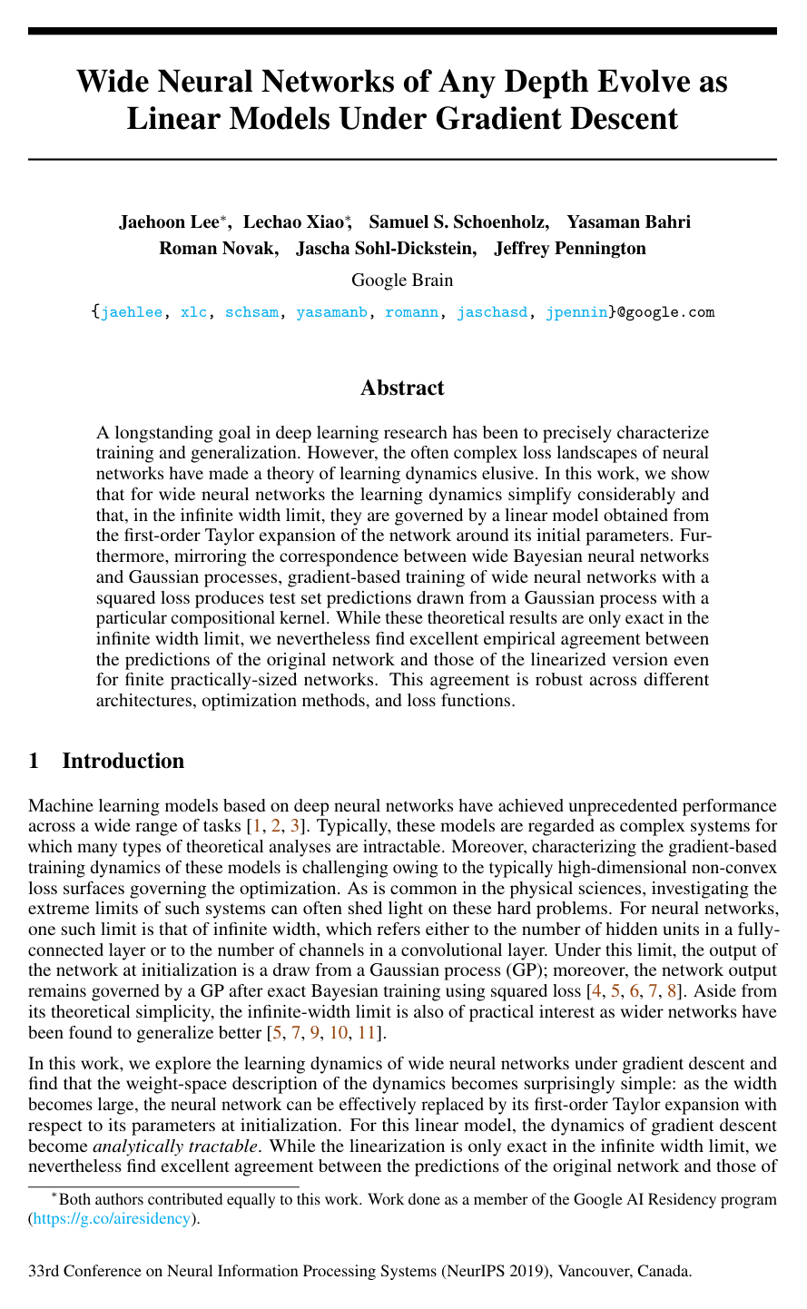
Wide neural networks of any depth evolve as linear models under gradient descent

Jaehoon LeeLechao XiaoSamuel S. SchoenholzYasaman BahriRoman NovakJascha Sohl-DicksteinJeffrey Pennington

article2019NeurIPS1,366 citations

Proves that deep neural networks evolve as linear models under gradient descent in the infinite-width limit, bridging complex neural network training dynamics with tractable Gaussian process theory and matching the empirical behavior of practical finite-width architectures.

Listen

Deep neural networks are central to modern artificial intelligence, yet understanding how their parameters evolve during training remains a major challenge due to complex, high-dimensional optimization surfaces. As organizations increasingly rely on deep learning for mission-critical applications, the lack of theoretical clarity regarding training dynamics and generalization introduces uncertainty and unpredictability in model behavior. To address this issue, the article investigates the extreme limit of network width—the number of hidden units or channels—to establish whether the training behavior of highly parameterized neural networks can be simplified and rigorously predicted.

The main objective of the article is to demonstrate theoretically and empirically that sufficiently wide neural networks evolve during gradient-based training as linear models derived from their initial state, and to show that their outputs follow predictable statistical distributions across training.

To evaluate this behavior, the authors combined formal mathematical proofs with extensive empirical simulations. They mathematically analyzed the training trajectories of wide networks under continuous and discrete gradient descent across both standard and specialized parameterizations. Experimentally, they tested multiple architectures—including fully-connected networks, convolutional networks, and practical Wide Residual Networks—on standard benchmark image datasets (MNIST and CIFAR-10) using various loss functions (mean squared error and cross-entropy) and optimization techniques like momentum and mini-batching.

The article establishes several key findings. First, as the width of a neural network approaches infinity, its gradient descent learning dynamics become mathematically equivalent to a linear model based on a first-order Taylor expansion around its initial parameters. Second, during training, individual internal weights move only a vanishingly small amount, yet their collective movement yields the exact target outputs. Third, for squared error loss, the training dynamics admit exact closed-form solutions where the network's predictive output distribution throughout training evolves as a Gaussian process governed by a deterministic kernel known as the Neural Tangent Kernel. Fourth, empirical experiments confirm that this linear approximation closely matches actual training dynamics, loss reduction, and classification accuracy even in practical, finite-width models (such as networks with widths or channel sizes between 512 and 8,192). Finally, the deviation between a finite network and its linearized counterpart decreases predictably at an inverse square-root rate relative to layer width, though this discrepancy tends to grow with larger dataset sizes.

These findings provide practical implications for model development and analysis. They demonstrate that very wide networks can be studied, diagnosed, and partly predicted using linear and kernel methods rather than opaque black-box heuristics. This can improve development timelines and performance evaluations by allowing closed-form calculations or simplified linear training rather than extensive empirical trial and error. Furthermore, the results clarify the fundamental distinction between standard gradient descent training and full Bayesian posterior sampling, illustrating that gradient-trained wide networks induce a distinct predictive distribution rather than sampling from a Bayesian model posterior.

For practitioners and researchers, the article suggests leveraging kernel methods and the released open-source software tools to study architectural trainability and generalization prior to heavy compute investments. Organizations can explore linearized models to diagnose baseline behavior on complex architectures. However, further research is recommended before fully replacing standard deep architectures with linear kernel equivalents, particularly to determine why performance gaps between finite and infinite models persist in certain designs (such as convolutional networks without pooling) and how to best manage scaling trade-offs as dataset sizes increase.

The conclusions are supported by robust proofs and consistent experimental validations across varied model setups, providing high confidence in the theoretical results for wide regimes. Nevertheless, stakeholders should note important boundary conditions: the exact mathematical equivalence applies strictly in the infinite-width limit with learning rates below a critical threshold. In practice, models trained with cross-entropy loss can show growing divergence in late-stage outputs, and real-world networks with narrower widths or specific non-pooling architectures may operate outside this linearized regime.

Google bayesian methods deep learning gaussian processes wide neural networks neural tangent kernel gradient descent

arXiv: 1902.06720

Paper: Neural Tangent Kernel: Convergence and Generalization in Neural Networks, Arthur Jacot et al. (2018). This foundational paper introduces the Neural Tangent Kernel (NTK) framework in the infinite-width limit, providing the direct mathematical basis upon which the source's linearized model and gradient flow equivalence are established.
Paper: Gradient Descent Provably Optimizes Over-parameterized Neural Networks, Simon S. Du et al. (2018). This work establishes that over-parameterized neural network parameters remain close to their initializations during gradient descent, laying essential analytical groundwork for analyzing wide networks as linearized models.
Paper: A Convergence Theory for Deep Learning via Over-Parameterization, Zeyuan Allen-Zhu et al. (2018). It proves polynomial-time global convergence for over-parameterized deep neural networks optimized via gradient descent by characterizing trajectories near initialization.
Paper: Exact solutions to the nonlinear dynamics of learning in deep linear neural networks, Andrew M. Saxe et al. (2014). This paper offers foundational exact solutions for learning dynamics in deep linear networks under gradient descent, motivating continuous-time analytical perspectives on network evolution.

Paper: Fourier Features Let Networks Learn High Frequency Functions in Low Dimensional Domains, Matthew Tancik et al. (2020). It applies the Neural Tangent Kernel perspective from wide network theory to diagnose spectral bias and introduces Fourier feature mappings to enable coordinate-based MLPs to fit high-frequency functions.
Paper: When and why PINNs fail to train: A neural tangent kernel perspective, Sifan Wang et al. (2020). This paper leverages the infinite-width Neural Tangent Kernel framework to analyze and overcome training failure modes and spectral bias in physics-informed neural networks.
Paper: There Will Be a Scientific Theory of Deep Learning, Jamie Simon et al. (2026). It synthesizes infinite-width 'lazy' kernel regimes with broader theoretical principles into an overarching physical framework of deep learning mechanics and optimization dynamics.

Cover for Wide neural networks of any depth evolve as linear models under gradient descent

Abstract

A longstanding goal in deep learning research has been to precisely characterize training and generalization. However, the often complex loss landscapes of neural networks have made a theory of learning dynamics elusive. In this work, we show that for wide neural networks the learning dynamics simplify considerably and that, in the infinite width limit, they are governed by a linear model obtained from the first-order Taylor expansion of the network around its initial parameters. Furthermore, mirroring the correspondence between wide Bayesian neural networks and Gaussian processes, gradient-based training of wide neural networks with a squared loss produces test set predictions drawn from a Gaussian process with a particular compositional kernel. While these theoretical results are only exact in the infinite width limit, we nevertheless find excellent empirical agreement between the predictions of the original network and those of the linearized version even for finite practically-sized networks. This agreement is robust across different architectures, optimization methods, and loss functions.

Topics

bayesian methods deep learning gaussian processes gaussians linear models network architecture optimization optimization problems test samples theoretical result

Keywords

wide neural networks neural tangent kernel gradient descent infinite width networks training dynamics gradient flow linear models Gaussian processes Taylor expansion

1 Introduction
1.1 Related work
2 Theoretical results
2.1 Notation and setup for architecture and training dynamics
2.2 Linearized networks have closed form training dynamics for parameters and outputs
2.3 Infinite width limit yields a Gaussian process
2.3.1 Gaussian processes from gradient descent training
2.4 Infinite width networks are linearized networks
2.5 Extensions to other optimizers, architectures, and losses
3 Experiments
4 Discussion
References
A Additional figures
B Extensions
B.1 Momentum
B.2 Multi-dimensional output and cross-entropy loss
C Neural Tangent kernel for ReLU\operatorname{ReLU} and erf\operatorname{erf}
D Gradient flow dynamics for training only the readout-layer
E Computing NTK and NNGP Kernel
F Results in function space for NTK parameterization transfer to standard parameterization
G Convergence of neural network to its linearization, and stability of NTK under gradient descent
G.1 Proof of Theorem
G.2 Proof of Theorem
G.3 Proof of Lemma
G.4 Remarks on NTK parameterization
H Bounding the discrepancy between the original and the linearized network: MSE loss
I Convergence of empirical kernel
J Details on Wide Residual Network

Knowls

Knowl 1 — Linearized Neural Network Model and Closed-Form Parameter and Output Dynamics under Squared Loss
model/method
For a neural network with parameters $\theta \in \mathbb{R}^p$ and initial parameter vector $\theta_0$ , the linearized neural network $f_t^{\text{lin}}(x) \in \mathbb{R}^k$ for an input $x \in \mathbb{R}^{n_0}$ is defined by its first-order Taylor expansion around $\theta_0$ :

$f_t^{\text{lin}}(x) \equiv f_0(x) + \left.\nabla_\theta f(x)\right|_{\theta=\theta_0} \omega_t,$

where $\omega_t \equiv \theta_t - \theta_0 \in \mathbb{R}^p$ represents the change in parameter values from initialization, and $f_0(x) \equiv f(x, \theta_0)$ is the initial output. For a dataset $\mathcal{D} = \{(x_i, y_i)\}_{i=1}^{|\mathcal{D}|}$ with inputs $\mathcal{X} = \{x_i\}$ and target labels $\mathcal{Y} = \{y_i\}$ , under continuous-time gradient flow with learning rate $\eta$ and mean-squared error (MSE) loss $\mathcal{L} = \frac{1}{2}\|f_t^{\text{lin}}(\mathcal{X}) - \mathcal{Y}\|_2^2$ , the dynamics of $\omega_t$ and $f_t^{\text{lin}}$ are given by:

$\dot{\omega}_t = -\eta \nabla_\theta f_0(\mathcal{X})^T \nabla_{f_t^{\text{lin}}(\mathcal{X})}\mathcal{L},$

$\dot{f}_t^{\text{lin}}(x) = -\eta \hat{\Theta}_0(x, \mathcal{X}) \nabla_{f_t^{\text{lin}}(\mathcal{X})}\mathcal{L},$

where $\hat{\Theta}_0(x, x') \equiv \nabla_\theta f_0(x) \nabla_\theta f_0(x')^T$ is the empirical Neural Tangent Kernel (NTK) at initialization, and $\hat{\Theta}_0 \equiv \hat{\Theta}_0(\mathcal{X}, \mathcal{X})$ . When $\hat{\Theta}_0$ is invertible, the gradient flow ODEs admit exact closed-form solutions for any time $t \ge 0$ :

$\omega_t = -\nabla_\theta f_0(\mathcal{X})^T \hat{\Theta}_0^{-1} \left(I - e^{-\eta \hat{\Theta}_0 t}\right)(f_0(\mathcal{X}) - \mathcal{Y}),$

$f_t^{\text{lin}}(\mathcal{X}) = \left(I - e^{-\eta \hat{\Theta}_0 t}\right)\mathcal{Y} + e^{-\eta \hat{\Theta}_0 t} f_0(\mathcal{X}).$

For an arbitrary evaluation point $x$ , the output decomposes as $f_t^{\text{lin}}(x) = \mu_t(x) + \gamma_t(x)$ , with:

$\mu_t(x) = \hat{\Theta}_0(x, \mathcal{X})\hat{\Theta}_0^{-1} \left(I - e^{-\eta \hat{\Theta}_0 t}\right)\mathcal{Y},$

$\gamma_t(x) = f_0(x) - \hat{\Theta}_0(x, \mathcal{X})\hat{\Theta}_0^{-1} \left(I - e^{-\eta \hat{\Theta}_0 t}\right)f_0(\mathcal{X}).$
Knowl 2 — Asymptotic Equivalence of Non-Linear Neural Network and Linearized Model Trajectories
theoretical result
Consider a fully connected feed-forward neural network of depth $L$ with identical hidden layer widths $n_1 = \dots = n_L = n$ , trained on dataset $(\mathcal{X}, \mathcal{Y})$ with mean squared loss. Let $\Theta \equiv \lim_{n \to \infty} \hat{\Theta}_0(\mathcal{X}, \mathcal{X})$ denote the analytic infinite-width Neural Tangent Kernel, and assume $\lambda_{\min}(\Theta) > 0$ . Define the critical learning rate threshold:

$\eta_{\text{critical}} \equiv \frac{2}{\lambda_{\min}(\Theta) + \lambda_{\max}(\Theta)}.$

If the learning rate satisfies $\eta < \eta_{\text{critical}}$ , then for any test input $x \in \mathbb{R}^{n_0}$ with $\|x\|_2 \le 1$ , under discrete gradient descent or continuous gradient flow, with probability arbitrarily close to 1 over random parameter initialization:

$\sup_{t \ge 0} \left\|f_t(x) - f_t^{\text{lin}}(x)\right\|_2 = O\left(n^{-1/2}\right),$

$\sup_{t \ge 0} \frac{\|\theta_t - \theta_0\|_2}{\sqrt{n}} = O\left(n^{-1/2}\right),$

$\sup_{t \ge 0} \left\|\hat{\Theta}_t - \hat{\Theta}_0\right\|_F = O\left(n^{-1/2}\right),$

as $n \to \infty$ , where $f_t(x)$ is the output of the full non-linear network, $f_t^{\text{lin}}(x)$ is the output of the first-order Taylor linearized model, $\theta_t$ is the parameter vector, and $\hat{\Theta}_t$ is the empirical tangent kernel matrix at time $t$ . As a result, the distribution over training trajectories of the non-linear network converges to that of the linearized model as $n \to \infty$ .
Knowl 3 — Gaussian Process Evolution of Predictive Distributions under Gradient Descent Training
theoretical result
Let an infinitely wide neural network be trained on a training dataset $(\mathcal{X}, \mathcal{Y})$ using continuous-time gradient descent with learning rate $\eta < \eta_{\text{critical}}$ on a mean squared error loss. Over the random draw of parameter initialization, the predictive function distribution evaluated on a test set $\mathcal{X}_T$ at time $t \ge 0$ converges in distribution as hidden layer width $n \to \infty$ to a Gaussian process $\mathcal{N}(\mu(\mathcal{X}_T), \Sigma(\mathcal{X}_T, \mathcal{X}_T))$ , with mean and covariance functions given by:

$\mu(\mathcal{X}_T) = \Theta(\mathcal{X}_T, \mathcal{X}) \Theta^{-1} \left(I - e^{-\eta \Theta t}\right) \mathcal{Y},$

$\Sigma(\mathcal{X}_T, \mathcal{X}_T) = K(\mathcal{X}_T, \mathcal{X}_T) + \Theta(\mathcal{X}_T, \mathcal{X})\Theta^{-1}\left(I - e^{-\eta \Theta t}\right) K \left(I - e^{-\eta \Theta t}\right) \Theta^{-1}\Theta(\mathcal{X}, \mathcal{X}_T) - \left(\Theta(\mathcal{X}_T, \mathcal{X})\Theta^{-1}\left(I - e^{-\eta \Theta t}\right) K(\mathcal{X}, \mathcal{X}_T) + \text{h.c.}\right),$

where $\Theta \equiv \Theta(\mathcal{X}, \mathcal{X})$ is the infinite-width Neural Tangent Kernel (NTK), $K \equiv K(\mathcal{X}, \mathcal{X})$ is the infinite-width Neural Network Gaussian Process (NNGP) kernel, and $\text{h.c.}$ denotes the Hermitian conjugate (transpose for real matrices). In the asymptotic training limit $t \to \infty$ , the output distribution converges to:

$\lim_{t \to \infty} \lim_{n \to \infty} f_t(x) \sim \mathcal{N}\left(\Theta(x, \mathcal{X})\Theta^{-1}\mathcal{Y}, \; K(x, x) + \Theta(x, \mathcal{X})\Theta^{-1} K \Theta^{-1}\Theta(\mathcal{X}, x) - \left(\Theta(x, \mathcal{X})\Theta^{-1} K(\mathcal{X}, x) + \text{h.c.}\right)\right).$

This distribution differs from the exact Bayesian posterior under the NNGP kernel $K$ , demonstrating that gradient descent training of all layers does not perform Bayesian posterior inference.
Knowl 4 — Bayesian Posterior Equivalence for Readout-Layer Only Optimization
theoretical result
When all hidden layer parameters $\theta^{\le L}$ of a neural network are kept frozen at their random Gaussian initialization and only the readout layer parameters $\theta^{L+1}$ are optimized using gradient flow with mean squared error loss $\mathcal{L} = \frac{1}{2}\|f(\mathcal{X}) - \mathcal{Y}\|_2^2$ , the model predictions on an arbitrary test input $x^*$ are Gaussian distributed over the ensemble of initializations for all $t \ge 0$ in the infinite-width limit $n_1, \dots, n_L \to \infty$ :

$\mathbb{E}[f_t(x^*)] = K(x^*, \mathcal{X}) K^{-1} \left(I - e^{-\eta K t}\right) \mathcal{Y},$

$\text{Var}[f_t(x^*)] = K(x^*, x^*) - K(x^*, \mathcal{X}) K^{-1} \left(I - e^{-2\eta K t}\right) K(x^*, \mathcal{X})^T,$

where $K \equiv K(\mathcal{X}, \mathcal{X})$ is the infinite-width NNGP covariance kernel. In the limit $t \to \infty$ , this predictive distribution converges to:

$\lim_{t \to \infty} f_t(x^*) \sim \mathcal{N}\left(K(x^*, \mathcal{X})K^{-1}\mathcal{Y}, \; K(x^*, x^*) - K(x^*, \mathcal{X})K^{-1}K(x^*, \mathcal{X})^T\right),$

which is identical to the exact Bayesian posterior predictive distribution of a Gaussian process with kernel $K$ . Thus, optimizing only the readout layer via gradient flow is mathematically equivalent to exact "sample-then-optimize" Bayesian posterior sampling.
Knowl 5 — Recursive Formulation of the NNGP and Neural Tangent Kernels
equation
For a deep feed-forward neural network with point-wise activation $\phi$ , weight variances $\sigma_w^2$ , and bias variances $\sigma_b^2$ , the infinite-width NNGP kernel $K^l(x, x')$ and Neural Tangent Kernel $\Theta^l(x, x')$ at layer $l \in \{1, \dots, L+1\}$ for inputs $x, x' \in \mathbb{R}^{n_0}$ are computed recursively as:

$K^l(x, x') = \tilde{K}^l(x, x') \otimes \text{Id}_{n_l}, \quad \Theta^l(x, x') = \tilde{\Theta}^l(x, x') \otimes \text{Id}_{n_l},$

with base cases at layer 1:

$\tilde{K}^1(x, x') = \tilde{\Theta}^1(x, x') = \sigma_w^2 \left(\frac{1}{n_0} x^T x'\right) + \sigma_b^2.$

For layers $l \ge 1$ , the recursive step is defined by:

$\tilde{K}^{l+1}(x, x') = \sigma_w^2 \mathcal{T}\left(\begin{pmatrix} \tilde{K}^l(x, x) & \tilde{K}^l(x, x') \\ \tilde{K}^l(x, x') & \tilde{K}^l(x', x') \end{pmatrix}\right) + \sigma_b^2,$

$\tilde{\Theta}^{l+1}(x, x') = \tilde{K}^{l+1}(x, x') + \sigma_w^2 \tilde{\Theta}^l(x, x') \dot{\mathcal{T}}\left(\begin{pmatrix} \tilde{K}^l(x, x) & \tilde{K}^l(x, x') \\ \tilde{K}^l(x, x') & \tilde{K}^l(x', x') \end{pmatrix}\right),$

where the dual activation operators $\mathcal{T}(\Sigma)$ and $\dot{\mathcal{T}}(\Sigma)$ for a $2 \times 2$ positive semi-definite covariance matrix $\Sigma$ are defined as expectations over $(u, v) \sim \mathcal{N}(0, \Sigma)$ :

$\mathcal{T}(\Sigma) = \mathbb{E}[\phi(u)\phi(v)], \quad \dot{\mathcal{T}}(\Sigma) = \mathbb{E}[\phi'(u)\phi'(v)].$
Knowl 6 — Analytic Dual Activation Kernels for ReLU and erf Nonlinearities
equation
For a $2 \times 2$ positive semi-definite covariance matrix $\Sigma = \begin{pmatrix} \Sigma_{11} & \Sigma_{12} \\ \Sigma_{12} & \Sigma_{22} \end{pmatrix}$ and angle $\theta = \arccos\left(\frac{\Sigma_{12}}{\sqrt{\Sigma_{11}\Sigma_{22}}}\right)$ , the dual activation functions $\mathcal{T}(\Sigma) = \mathbb{E}_{(u,v)\sim\mathcal{N}(0,\Sigma)}[\phi(u)\phi(v)]$ and $\dot{\mathcal{T}}(\Sigma) = \mathbb{E}_{(u,v)\sim\mathcal{N}(0,\Sigma)}[\phi'(u)\phi'(v)]$ admit closed forms for rectified linear unit (ReLU) and error function (erf) activations:
1. For $\phi(x) = \max(x, 0)$ (ReLU):
$\mathcal{T}(\Sigma) = \frac{1}{2\pi} \sqrt{\Sigma_{11}\Sigma_{22}} \left(\sin\theta + (\pi - \theta)\cos\theta\right) = \frac{1}{2\pi}\left(\sqrt{\Sigma_{11}\Sigma_{22} - \Sigma_{12}^2} + (\pi - \theta)\Sigma_{12}\right),$

$\dot{\mathcal{T}}(\Sigma) = \frac{1}{2\pi}(\pi - \theta).$
1. For $\phi(x) = \text{erf}(x)$ :
$\mathcal{T}(\Sigma) = \frac{2}{\pi} \arcsin\left(\frac{2\Sigma_{12}}{\sqrt{(1 + 2\Sigma_{11})(1 + 2\Sigma_{22})}}\right),$

$\dot{\mathcal{T}}(\Sigma) = \frac{4}{\pi} \det(I + 2\Sigma)^{-1/2} = \frac{4}{\pi \sqrt{(1 + 2\Sigma_{11})(1 + 2\Sigma_{22}) - 4\Sigma_{12}^2}}.$
Knowl 7 — Dynamical Equivalence between Standard and NTK Parameterizations under Scaled Learning Rates
theoretical result
The standard network parameterization defines weights $W_{ij}^l \sim \mathcal{N}\left(0, \frac{\sigma_w^2}{n_l}\right)$ and biases $b_j^l \sim \mathcal{N}(0, \sigma_b^2)$ with global gradient descent learning rate $\eta_{\text{std}} = \frac{\eta_0}{n_{\max}}$ , where $n_{\max} = \max_l n_l$ . The NTK parameterization defines $W_{ij}^l = \frac{\sigma_w}{\sqrt{n_l}} \omega_{ij}^l$ and $b_j^l = \sigma_b \beta_j^l$ with trainable variables initialized as standard Gaussians $\omega_{ij}^l, \beta_j^l \sim \mathcal{N}(0, 1)$ .

While the represented function at initialization is identical in both parameterizations, the training trajectories under gradient descent are equivalent if and only if layer-dependent learning rates $\eta_{\text{NTK}, w}^l$ and $\eta_{\text{NTK}, b}^l$ are applied in the NTK parameterization:

$\eta_{\text{NTK}, w}^l = \frac{n_l}{n_{\max}\sigma_w^2} \eta_0, \quad \eta_{\text{NTK}, b}^l = \frac{1}{n_{\max}\sigma_b^2} \eta_0.$

Consequently, parameter-space linearization, stability of the tangent kernel, and convergence to Gaussian process dynamics hold for networks in both standard parameterization and NTK parameterization as hidden layer widths approach infinity.
Knowl 8 — Linearized Network Dynamics for Momentum Optimization and Cross-Entropy Loss
model/method
The linearization of neural network outputs $f_t^{\text{lin}}(x)$ extends beyond gradient descent with squared error to momentum optimizers and general multi-output loss functions:
1. For discrete momentum updates $\theta_{i+1} = \theta_i + \beta(\theta_i - \theta_{i-1}) - \eta \left.\nabla_\theta \mathcal{L}\right|_{\theta=\theta_i}$ , the discrete function-space update is:
$f_{i+1}^{\text{lin}}(x) = f_i^{\text{lin}}(x) - \eta \hat{\Theta}_0(x, \mathcal{X}) \nabla_{f_i^{\text{lin}}(\mathcal{X})}\mathcal{L} + \beta\left(f_i^{\text{lin}}(x) - f_{i-1}^{\text{lin}}(x)\right).$

In continuous time with rescaled time $t = i\sqrt{\eta}$ and friction coefficient $\tilde{\beta} = \frac{\beta - 1}{\sqrt{\eta}}$ , the dynamics follow the second-order ODE:

$\ddot{f}_t^{\text{lin}}(x) = \tilde{\beta} \dot{f}_t^{\text{lin}}(x) - \hat{\Theta}_0(x, \mathcal{X}) \nabla_{f_t^{\text{lin}}(\mathcal{X})}\mathcal{L}.$
1. For multi-class classification with target one-hot vectors $\mathcal{Y}$ under cross-entropy loss $\mathcal{L}(f, y) = -\sum_i y_i \log \sigma(f_i)$ where $\sigma(f)_i = \frac{\exp(f_i)}{\sum_j \exp(f_j)}$ , the linearized gradient flow ODEs are:
$\dot{f}_t^{\text{lin}}(\mathcal{X}) = -\eta \hat{\Theta}_0(\mathcal{X}, \mathcal{X}) \left(\sigma\left(f_t^{\text{lin}}(\mathcal{X})\right) - \mathcal{Y}\right),$

$\dot{f}_t^{\text{lin}}(x) = -\eta \hat{\Theta}_0(x, \mathcal{X}) \left(\sigma\left(f_t^{\text{lin}}(\mathcal{X})\right) - \mathcal{Y}\right),$

which can be integrated numerically as an initial value problem using standard ODE solvers.
Knowl 9 — Empirical Scaling of Weight Changes, Kernel Stability, and Linearized Model Tracking
empirical result
Empirical evaluations on MNIST and CIFAR-10 across fully-connected networks, convolutional networks, and Wide Residual Networks (WRNs with 1024 channels) confirm that:
1. Parameter changes across $T$ training steps scale as $\frac{\|\theta_T^l - \theta_0^l\|_F}{\|\theta_0^l\|_F} = O\left(n^{-1/2}\right)$ for input and output layers, and as $O\left(n^{-1}\right)$ for intermediate hidden layers of width $n$ .
2. The relative drift of the empirical tangent kernel during training scales as $\frac{\|\hat{\Theta}_T^{(n)} - \hat{\Theta}_0^{(n)}\|_F}{\|\hat{\Theta}_0^{(n)}\|_F} = O(n^{-1})$ , whereas the finite-width empirical kernel deviates from the infinite-width analytic kernel by $\frac{\|\hat{\Theta}_0^{(n)} - \Theta\|_F}{\|\Theta\|_F} = O\left(n^{-1/2}\right)$ .
3. Because the training-induced kernel change $O(n^{-1})$ is smaller than the initialization discrepancy $O(n^{-1/2})$ , linearized dynamics computed using the empirical kernel $\hat{\Theta}_0$ track finite-width non-linear network outputs, training loss, and test accuracy significantly closer than dynamics computed using the infinite-width analytic kernel $\Theta$ .

Coverage note — None was omitted; all primary theoretical results, kernel definitions, closed-form formulas, algorithmic extensions, and empirical findings have been captured.

References

1.Alex Krizhevsky, Ilya Sutskever, and Geoffrey E Hinton. Imagenet classification with deep convolutional neural networks. In Advances in Neural Information Processing Systems. 2012.
2.Kaiming He, Xiangyu Zhang, Shaoqing Ren, and Jian Sun. Deep residual learning for image recognition. In Conference on Computer Vision and Pattern Recognition, pages 770–778, 2016.
3.Jacob Devlin, Ming-Wei Chang, Kenton Lee, and Kristina Toutanova. Bert: Pre-training of deep bidirectional transformers for language understanding. arXiv preprint arXiv:1810.04805, 2018.
4.Radford M. Neal. Priors for infinite networks (tech. rep. no. crg-tr-94-1). University of Toronto, 1994.
5.Jaehoon Lee, Yasaman Bahri, Roman Novak, Sam Schoenholz, Jeffrey Pennington, and Jascha Sohl-dickstein. Deep neural networks as gaussian processes. In International Conference on Learning Representations, 2018.
6.Alexander G. de G. Matthews, Jiri Hron, Mark Rowland, Richard E. Turner, and Zoubin Ghahramani. Gaussian process behaviour in wide deep neural networks. In International Conference on Learning Representations, 4 2018. URL https://openreview.net/forum?id=H1-nGgWC-.
7.Roman Novak, Lechao Xiao, Jaehoon Lee, Yasaman Bahri, Greg Yang, Jiri Hron, Daniel A. Abolafia, Jeffrey Pennington, and Jascha Sohl-Dickstein. Bayesian deep convolutional networks with many channels are gaussian processes. In International Conference on Learning Representations, 2019.
8.Adrià Garriga-Alonso, Laurence Aitchison, and Carl Edward Rasmussen. Deep convolutional networks as shallow gaussian processes. In International Conference on Learning Representations, 2019.
9.Behnam Neyshabur, Ryota Tomioka, and Nathan Srebro. In search of the real inductive bias: On the role of implicit regularization in deep learning. In International Conference on Learning Representations workshop track, 2015.
10.Roman Novak, Yasaman Bahri, Daniel A. Abolafia, Jeffrey Pennington, and Jascha Sohl-Dickstein. Sensitivity and generalization in neural networks: an empirical study. In International Conference on Learning Representations, 2018.
11.Behnam Neyshabur, Zhiyuan Li, Srinadh Bhojanapalli, Yann LeCun, and Nathan Srebro. The role of over-parametrization in generalization of neural networks. In International Conference on Learning Representations, 2019.
12.Alexander G. de G. Matthews, Jiri Hron, Richard E. Turner, and Zoubin Ghahramani. Sample-then-optimize posterior sampling for bayesian linear models. In NeurIPS Workshop on Advances in Approximate Bayesian Inference, 2017. URL http://approximateinference.org/2017/accepted/MatthewsEtAl2017.pdf.
13.Arthur Jacot, Franck Gabriel, and Clement Hongler. Neural tangent kernel: Convergence and generalization in neural networks. In Advances in Neural Information Processing Systems, 2018.
14.Sergey Zagoruyko and Nikos Komodakis. Wide residual networks. In British Machine Vision Conference, 2016.
15.Roman Novak, Lechao Xiao, Jiri Hron, Jaehoon Lee, Alexander A. Alemi, Jascha Sohl-Dickstein, and Samuel S. Schoenholz. Neural tangents: Fast and easy infinite neural networks in python. https://github.com/google/neural-tangents, https://arxiv.org/abs/1912.02803, 2019.
16.Amit Daniely, Roy Frostig, and Yoram Singer. Toward deeper understanding of neural networks: The power of initialization and a dual view on expressivity. In Advances In Neural Information Processing Systems, 2016.
17.Amit Daniely. SGD learns the conjugate kernel class of the network. In Advances in Neural Information Processing Systems, 2017.
18.Andrew M Saxe, James L McClelland, and Surya Ganguli. Exact solutions to the nonlinear dynamics of learning in deep linear neural networks. In International Conference on Learning Representations, 2014.
19.Simon S Du, Jason D Lee, Haochuan Li, Liwei Wang, and Xiyu Zhai. Gradient descent finds global minima of deep neural networks. In International Conference on Machine Learning, 2019.
20.Zeyuan Allen-Zhu, Yuanzhi Li, and Zhao Song. A convergence theory for deep learning via over-parameterization. In International Conference on Machine Learning, 2019.
21.Zeyuan Allen-Zhu, Yuanzhi Li, and Zhao Song. On the convergence rate of training recurrent neural networks. arXiv preprint arXiv:1810.12065, 2018.
22.Difan Zou, Yuan Cao, Dongruo Zhou, and Quanquan Gu. Stochastic gradient descent optimizes over-parameterized deep relu networks. Machine Learning, 2019.
23.Song Mei, Andrea Montanari, and Phan-Minh Nguyen. A mean field view of the landscape of two-layer neural networks. Proceedings of the National Academy of Sciences, 115(33): E7665–E7671, 2018.
24.Lenaic Chizat and Francis Bach. On the global convergence of gradient descent for over-parameterized models using optimal transport. In Advances in neural information processing systems, 2018.
25.Grant M Rotskoff and Eric Vanden-Eijnden. Parameters as interacting particles: long time convergence and asymptotic error scaling of neural networks. In Advances in neural information processing systems, 2018.
26.Justin Sirignano and Konstantinos Spiliopoulos. Mean field analysis of neural networks. arXiv preprint arXiv:1805.01053, 2018.
27.Xavier Glorot and Yoshua Bengio. Understanding the difficulty of training deep feedforward neural networks. In International Conference on Artificial Intelligence and Statistics, pages 249–256, 2010.
28.Lenaic Chizat, Edouard Oyallon, and Francis Bach. On lazy training in differentiable programming. arXiv preprint arXiv:1812.07956, 2018.
29.Twan van Laarhoven. L2 regularization versus batch and weight normalization. arXiv preprint arXiv:1706.05350, 2017.
30.Tero Karras, Timo Aila, Samuli Laine, and Jaakko Lehtinen. Progressive growing of GANs for improved quality, stability, and variation. In International Conference on Learning Representations, 2018.
31.Daniel S. Park, Jascha Sohl-Dickstein, Quoc V. Le, and Samuel L. Smith. The effect of network width on stochastic gradient descent and generalization: an empirical study. In International Conference on Machine Learning, 2019.
32.Ben Poole, Subhaneil Lahiri, Maithra Raghu, Jascha Sohl-Dickstein, and Surya Ganguli. Exponential expressivity in deep neural networks through transient chaos. In Advances In Neural Information Processing Systems, pages 3360–3368, 2016.
33.Samuel S Schoenholz, Justin Gilmer, Surya Ganguli, and Jascha Sohl-Dickstein. Deep information propagation. International Conference on Learning Representations, 2017.
34.Lechao Xiao, Yasaman Bahri, Jascha Sohl-Dickstein, Samuel Schoenholz, and Jeffrey Pennington. Dynamical isometry and a mean field theory of CNNs: How to train 10,000-layer vanilla convolutional neural networks. In International Conference on Machine Learning, 2018.
35.Ge Yang and Samuel Schoenholz. Mean field residual networks: On the edge of chaos. In Advances in Neural Information Processing Systems. 2017.
36.Alexander G de G Matthews, Mark Rowland, Jiri Hron, Richard E Turner, and Zoubin Ghahramani. Gaussian process behaviour in wide deep neural networks. arXiv preprint arXiv:1804.11271, 9 2018.
37.Greg Yang. Scaling limits of wide neural networks with weight sharing: Gaussian process behavior, gradient independence, and neural tangent kernel derivation. arXiv preprint arXiv:1902.04760, 2019.
38.Sever Silvestru Dragomir. Some Gronwall type inequalities and applications. Nova Science Publishers New York, 2003.
39.Minmin Chen, Jeffrey Pennington, and Samuel Schoenholz. Dynamical isometry and a mean field theory of RNNs: Gating enables signal propagation in recurrent neural networks. In International Conference on Machine Learning, 2018.
40.Greg Yang, Jeffrey Pennington, Vinay Rao, Jascha Sohl-Dickstein, and Samuel S. Schoenholz. A mean field theory of batch normalization. In International Conference on Learning Representations, 2019.
41.Roy Frostig, Peter Hawkins, Matthew Johnson, Chris Leary, and Dougal Maclaurin. JAX: Autograd and XLA. www.github.com/google/jax, 2018.
42.Martín Abadi, Paul Barham, Jianmin Chen, Zhifeng Chen, Andy Davis, Jeffrey Dean, Matthieu Devin, Sanjay Ghemawat, Geoffrey Irving, Michael Isard, et al. Tensorflow: A system for large-scale machine learning. In 12th USENIX Symposium on Operating Systems Design and Implementation (OSDI 16), 2016.
43.Chiyuan Zhang, Samy Bengio, and Yoram Singer. Are all layers created equal? arXiv preprint arXiv:1902.01996, 2019.
44.Ning Qian. On the momentum term in gradient descent learning algorithms. Neural networks, 12(1):145–151, 1999.
45.Weijie Su, Stephen Boyd, and Emmanuel Candes. A differential equation for modeling nesterov’s accelerated gradient method: Theory and insights. In Advances in Neural Information Processing Systems, pages 2510–2518, 2014.
46.Youngmin Cho and Lawrence K Saul. Kernel methods for deep learning. In Advances in neural information processing systems, 2009.
47.Christopher KI Williams. Computing with infinite networks. In Advances in neural information processing systems, pages 295–301, 1997.
48.Roman Vershynin. Introduction to the non-asymptotic analysis of random matrices. arXiv preprint arXiv:1011.3027, 2010.

Citation

MLA

Lee, J., et al. “Wide Neural Networks of Any Depth Evolve as Linear Models Under Gradient Descent ^*”. Journal of Statistical Mechanics: Theory and Experiment, vol. 2020, no. 12, 2020, p. 124002, https://doi.org/10.1088/1742-5468/abc62b.

APA

Lee, J., Xiao, L., Schoenholz, S. S., Bahri, Y., Novak, R., Sohl-Dickstein, J., & Pennington, J. (2020). Wide neural networks of any depth evolve as linear models under gradient descent ^*. Journal of Statistical Mechanics: Theory and Experiment, 2020(12), 124002. https://doi.org/10.1088/1742-5468/abc62b

Chicago

Lee, J., L. Xiao, S. S. Schoenholz, et al. 2020. “Wide Neural Networks of Any Depth Evolve as Linear Models Under Gradient Descent ^*”. Journal of Statistical Mechanics: Theory and Experiment 2020 (12): 124002. https://doi.org/10.1088/1742-5468/abc62b.

Harvard

Lee, J. et al. (2020) “Wide neural networks of any depth evolve as linear models under gradient descent ^*”, Journal of Statistical Mechanics: Theory and Experiment, 2020(12), p. 124002. Available at: https://doi.org/10.1088/1742-5468/abc62b.

Vancouver

1. Lee J, Xiao L, Schoenholz SS, Bahri Y, Novak R, Sohl-Dickstein J, Pennington J (2020) Wide neural networks of any depth evolve as linear models under gradient descent ^*. Journal of Statistical Mechanics: Theory and Experiment 2020:124002

BibTeX

@article{Lee_2020, title={Wide neural networks of any depth evolve as linear models under gradient descent
                    <sup>*</sup>}, volume={2020}, ISSN={1742-5468}, url={http://dx.doi.org/10.1088/1742-5468/abc62b}, DOI={10.1088/1742-5468/abc62b}, number={12}, journal={Journal of Statistical Mechanics: Theory and Experiment}, publisher={IOP Publishing}, author={Lee, Jaehoon and Xiao, Lechao and Schoenholz, Samuel S and Bahri, Yasaman and Novak, Roman and Sohl-Dickstein, Jascha and Pennington, Jeffrey}, year={2020}, month=Dec, pages={124002} }

Metadata:Crossref

Access the Paper

This paper is available from its original source. Click below to access the PDF.

Open PDF

License: Published with permission

Wide neural networks of any depth evolve as linear models under gradient descent

Abstract

Topics

Keywords

Table of Contents

Knowls

Knowl 1 — Linearized Neural Network Model and Closed-Form Parameter and Output Dynamics under Squared Loss

Knowl 2 — Asymptotic Equivalence of Non-Linear Neural Network and Linearized Model Trajectories

Knowl 3 — Gaussian Process Evolution of Predictive Distributions under Gradient Descent Training

Knowl 4 — Bayesian Posterior Equivalence for Readout-Layer Only Optimization

Knowl 5 — Recursive Formulation of the NNGP and Neural Tangent Kernels

Knowl 6 — Analytic Dual Activation Kernels for ReLU and erf Nonlinearities

Knowl 7 — Dynamical Equivalence between Standard and NTK Parameterizations under Scaled Learning Rates

Knowl 8 — Linearized Network Dynamics for Momentum Optimization and Cross-Entropy Loss

Knowl 9 — Empirical Scaling of Weight Changes, Kernel Stability, and Linearized Model Tracking

References

Citation

BibTeX

Access the Paper