On First-Order Meta-Learning Algorithms

Alex NicholJoshua AchiamJohn Schulman

article2018arXiv2,658 citations

Introduces Reptile, a computationally efficient first-order meta-learning algorithm that avoids expensive second-order derivatives in MAML while matching its few-shot classification performance, supported by theoretical analysis explaining how first-order updates find effective initializations across tasks.

Listen

Machine learning models typically require large amounts of data to reach strong performance on new tasks, while humans can often learn from just a few examples. This gap motivates meta-learning methods that aim to produce agents capable of rapid adaptation to previously unseen tasks drawn from a distribution of related problems. The article examines a family of first-order algorithms that learn a parameter initialization optimized for quick fine-tuning, avoiding the computational cost of second-order derivatives required by full MAML.

The work set out to analyze why first-order approximations perform well, introduce a simpler algorithm called Reptile, and provide both theoretical insight and practical guidance for few-shot learning. The authors combine Taylor-series analysis of gradient updates with experiments on standard benchmarks. They evaluate on Omniglot and Mini-ImageNet few-shot classification tasks using convolutional networks, plus a controlled one-dimensional sine-wave regression problem, comparing MAML, first-order MAML, and Reptile under consistent architectures and optimizers.

The analysis shows that both first-order MAML and Reptile optimize not only the average loss across tasks but also the inner product of gradients computed on different minibatches within the same task, thereby improving within-task generalization. On Mini-ImageNet, Reptile with transduction reaches 49.97 % accuracy in the 1-shot 5-way setting and 65.99 % in the 5-shot setting, matching or slightly exceeding first-order MAML. On Omniglot the three methods perform similarly, with transduction providing a consistent boost. Reptile requires no explicit train-test split within each task and is simpler to implement than full MAML.

These results indicate that computationally lighter first-order methods can deliver performance comparable to more expensive second-order approaches on established few-shot benchmarks, lowering barriers to applying meta-learning at larger scale. The theoretical view also helps explain why standard pre-training followed by fine-tuning often succeeds. Practitioners can therefore consider Reptile as a practical baseline when second-order information is prohibitive.

Further work is warranted to adapt Reptile to reinforcement learning, test deeper networks, add regularization to close the train-test gap, and explore few-shot density estimation. The Taylor approximation underlying the analysis holds only for modest step sizes and iteration counts, and empirical gains remain sensitive to inner-loop batching choices; readers should therefore validate hyper-parameters on their specific data regime before large-scale deployment.

OpenAI adaptive algorithms classification meta-learning Meta-Learning First-Order MAML Reptile

arXiv: 1803.02999 openai/supervised-reptile

Paper: Model-Agnostic Meta-Learning for Fast Adaptation of Deep Networks, Chelsea Finn et al. (2017). It introduces Model-Agnostic Meta-Learning (MAML), providing the primary foundation, objective, and second-order optimization baseline that Reptile and first-order meta-learning algorithms analyze and simplify.
Paper: Optimization as a Model for Few-Shot Learning, S. Ravi et al. (2017). It frames few-shot learning directly as an optimization problem and establishes key benchmark protocols on Mini-ImageNet that this work adopts.
Paper: Learning to learn by gradient descent by gradient descent, Marcin Andrychowicz et al. (2016). It establishes the modern foundation of learning to optimize via gradient descent across tasks, providing conceptual background for gradient-based meta-learning.
Paper: Prototypical Networks for Few-shot Learning, Jake Snell et al. (2017). It establishes core few-shot episodic evaluation benchmarks and standard comparison baselines on Omniglot and Mini-ImageNet used throughout the paper.
Paper: Matching Networks for One Shot Learning, Oriol Vinyals et al. (2016). It formalizes episodic meta-learning for one-shot visual recognition that underpins the experimental setups and problem formulation in this paper.
Paper: Learning to Compare: Relation Network for Few-Shot Learning, Flood Sung et al. (2017). It provides foundational metric-learning and episodic training paradigms for few-shot image classification evaluated alongside gradient-based meta-learning methods.

Paper: Gradient Surgery for Multi-Task Learning, Tianhe Yu et al. (2020). It builds directly upon the dynamics of multi-task gradient alignment studied in first-order meta-learning by introducing gradient projection surgery to resolve destructive task conflicts.

Cover for On First-Order Meta-Learning Algorithms

Abstract

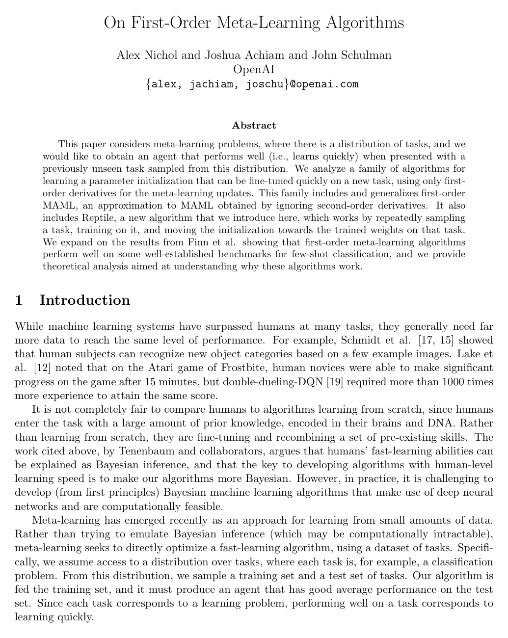
This paper considers meta-learning problems, where there is a distribution of tasks, and we would like to obtain an agent that performs well (i.e., learns quickly) when presented with a previously unseen task sampled from this distribution. We analyze a family of algorithms for learning a parameter initialization that can be fine-tuned quickly on a new task, using only first-order derivatives for the meta-learning updates. This family includes and generalizes first-order MAML, an approximation to MAML obtained by ignoring second-order derivatives. It also includes Reptile, a new algorithm that we introduce here, which works by repeatedly sampling a task, training on it, and moving the initialization towards the trained weights on that task. We expand on the results from Finn et al. showing that first-order meta-learning algorithms perform well on some well-established benchmarks for few-shot classification, and we provide theoretical analysis aimed at understanding why these algorithms work.

Topics

adaptive algorithms classification meta-learning optimization problems classification models efficient algorithm online learning

Keywords

Meta-Learning First-Order MAML Reptile Few-Shot Classification Gradient Descent Initialization Inner Loop Outer Loop Mini-ImageNet Omniglot

1 Introduction
2 Meta-Learning an Initialization
3 Reptile
4 Case Study: One-Dimensional Sine Wave Regression
5 Analysis
5.1 Leading Order Expansion of the Update
5.2 Finding a Point Near All Solution Manifolds
6 Experiments
6.1 Few-Shot Classification
6.2 Comparing Different Inner-Loop Gradient Combinations
6.3 Overlap Between Inner-Loop Mini-Batches
7 Discussion
8 Future Work
References
A Hyper-parameters

Knowls

Knowl 1 — Reptile Meta-Learning Algorithm
algorithm
Reptile is a first-order gradient-based meta-learning algorithm that learns an initial parameter vector $\phi$ for a parameterized model such that fine-tuning on a new, previously unseen task sampled from the same task distribution requires only a small number of gradient steps to generalize well.

In each meta-iteration of serial Reptile, a task $\tau$ is sampled from task distribution $p(\tau)$ . The model parameters $\phi$ are updated by executing $k$ consecutive steps of stochastic gradient descent (or an optimizer such as Adam) on the task loss $L_\tau$ , yielding adapted parameter vector $\tilde{\phi} = U_\tau^k(\phi)$ . The meta-parameters are then interpolated towards $\tilde{\phi}$ : $\phi \leftarrow \phi + \epsilon (\tilde{\phi} - \phi)$ where $\epsilon \in (0, 1]$ is the outer-loop step size.

In the batched (parallel) version, $n$ tasks $\{\tau_i\}_{i=1}^n$ are evaluated in parallel at each meta-iteration, performing $k$ inner steps on each task to yield $\tilde{\phi}_i = U_{\tau_i}^k(\phi)$ , and updating the initialization by averaging the task displacements: $\phi \leftarrow \phi + \frac{\epsilon}{n} \sum_{i=1}^n (\tilde{\phi}_i - \phi)$
Input: Initial parameter vector $\phi$ , outer step size $\epsilon$ , inner step size $\alpha$ , inner steps $k$ , task distribution $p(\tau)$
for iteration = 1, 2, ... do
    Sample task $\tau \sim p(\tau)$ with loss function $L_\tau$
    Initialize $\tilde{\phi} \leftarrow \phi$
    for step = 1, 2, ..., $k$ do
        Sample minibatch from task $\tau$
        Compute gradient $g \leftarrow \nabla_{\tilde{\phi}} L_\tau(\tilde{\phi})$
        Update inner parameters $\tilde{\phi} \leftarrow \tilde{\phi} - \alpha g$
    end for
    Update meta-parameters $\phi \leftarrow \phi + \epsilon (\tilde{\phi} - \phi)$
end for
Knowl 2 — Leading-Order Taylor Expansion of Meta-Learning Gradients
theoretical result
Approximating the inner-loop parameter trajectory of SGD with inner step size $\alpha$ via a Taylor series reveals the leading-order structure of the expected meta-gradients for MAML, First-Order MAML (FOMAML), and Reptile. Over a sequence of $k \ge 2$ inner-loop loss functions $L_1, L_2, \dots, L_k$ (e.g., losses on different minibatches from a sampled task), let $\phi_1$ denote the initial parameter vector, $\bar{g}_i = \nabla_{\phi_1} L_i(\phi_1)$ the initial gradients, and $\bar{H}_i = \nabla^2_{\phi_1} L_i(\phi_1)$ the initial Hessians.

The expected meta-gradients decompose to order $O(\alpha)$ as: $\mathbb{E}[g_{\text{MAML}}] = (1)\,\text{AvgGrad} - 2(k - 1)\alpha \,\text{AvgGradInner} + O(\alpha^2)$ $\mathbb{E}[g_{\text{FOMAML}}] = (1)\,\text{AvgGrad} - (k - 1)\alpha \,\text{AvgGradInner} + O(\alpha^2)$ $\mathbb{E}[g_{\text{Reptile}}] = (k)\,\text{AvgGrad} - \frac{1}{2} k(k - 1)\alpha \,\text{AvgGradInner} + O(\alpha^2)$

where: $\text{AvgGrad} = \mathbb{E}_{\tau, 1}[\bar{g}_1]$ $\text{AvgGradInner} = \mathbb{E}_{\tau, 1, 2}[\bar{H}_2 \bar{g}_1] = \frac{1}{2} \mathbb{E}_{\tau, 1, 2}\left[\nabla_{\phi_1}(\bar{g}_1 \cdot \bar{g}_2)\right]$

For any fixed $k \ge 2$ , the ratio of the coefficient of $\text{AvgGradInner}$ to that of $\text{AvgGrad}$ follows the ordering $\text{MAML} > \text{FOMAML} > \text{Reptile}$ . In all three algorithms, this ratio grows linearly with both the inner step size $\alpha$ and the number of iterations $k$ , provided $\alpha k$ is sufficiently small.
Knowl 3 — Within-Task Generalization via AvgGradInner and Joint Optimization via AvgGrad
definition
In gradient-based meta-learning objectives for initialization $\phi$ , the expected update decomposes into two distinct mathematical terms:
1. $\text{AvgGrad} = \mathbb{E}_{\tau, 1}[\nabla_\phi L_{\tau, 1}(\phi)]$ : The negative direction $-\text{AvgGrad}$ corresponds to standard joint training, driving parameters $\phi$ toward the minimizer of the average task loss $\mathbb{E}_\tau[L_\tau(\phi)]$ .
2. $\text{AvgGradInner} = \frac{1}{2}\mathbb{E}_{\tau, 1, 2}\left[\nabla_\phi (\nabla_\phi L_{\tau, 1}(\phi) \cdot \nabla_\phi L_{\tau, 2}(\phi))\right]$ : The negative direction $-\text{AvgGradInner}$ is the gradient of the expected inner product between gradients evaluated on two independent minibatches $1$ and $2$ drawn from the same task $\tau$ .
Moving in the direction of $-\text{AvgGradInner}$ maximizes the inner product $\nabla_\phi L_{\tau, 1}(\phi) \cdot \nabla_\phi L_{\tau, 2}(\phi)$ . When gradients across different batches within a task have positive dot products, performing a gradient step on one batch improves the model's loss on other batches, directly driving fast within-task generalization.
Knowl 4 — First-Order Model-Agnostic Meta-Learning (FOMAML) Formulation
algorithm
Model-Agnostic Meta-Learning (MAML) optimizes an initialization $\phi$ by minimizing $\mathbb{E}_\tau[L_{\tau, B}(U_{\tau, A}(\phi))]$ , where $U_{\tau, A}(\phi)$ denotes $k$ gradient updates on a task training set $A$ , and $L_{\tau, B}$ evaluates loss on a task validation set $B$ . The full MAML gradient is: $g_{\text{MAML}} = U'_{\tau, A}(\phi) \nabla_{\tilde{\phi}} L_{\tau, B}(\tilde{\phi})$ where $\tilde{\phi} = U_{\tau, A}(\phi)$ and $U'_{\tau, A}(\phi) = \prod_{j=1}^{k-1} (I - \alpha \nabla^2 L_{\tau, j}(\phi_j))$ is the Jacobian of the inner-loop update.

First-Order MAML (FOMAML) approximates this Jacobian by the identity matrix ( $U'_{\tau, A}(\phi) \approx I$ ), omitting all second-derivative terms. The outer-loop gradient is computed directly as the loss gradient evaluated at the adapted parameters $\tilde{\phi}$ on validation set $B$ : $g_{\text{FOMAML}} = \nabla_{\tilde{\phi}} L_{\tau, B}(\tilde{\phi})$
Input: Initial parameters $\phi$ , outer step size $\beta$ , inner step size $\alpha$ , inner steps $k$ , task distribution $p(\tau)$
for iteration = 1, 2, ... do
    Sample task $\tau \sim p(\tau)$
    Partition task data into disjoint sets $A$ and $B$
    Initialize $\tilde{\phi} \leftarrow \phi$
    for step = 1, 2, ..., $k$ do
        Compute inner gradient on set $A$ : $g \leftarrow \nabla_{\tilde{\phi}} L_{\tau, A}(\tilde{\phi})$
        Update inner parameters: $\tilde{\phi} \leftarrow \tilde{\phi} - \alpha g$
    end for
    Compute meta-gradient on set $B$ : $g_{\text{FOMAML}} \leftarrow \nabla_{\tilde{\phi}} L_{\tau, B}(\tilde{\phi})$
    Update initialization: $\phi \leftarrow \phi - \beta g_{\text{FOMAML}}$
end for
Knowl 5 — Geometric Characterization of Reptile as Distance Minimization to Task Solution Manifolds
theoretical result
Let $W_\tau \subset \mathbb{R}^d$ denote the manifold of optimal parameter vectors that minimize the loss for task $\tau$ . Reptile can be interpreted geometrically as performing stochastic gradient descent on the expected squared Euclidean distance from the initialization $\phi$ to each task's solution manifold: $\min_\phi \mathbb{E}_\tau \left[ \frac{1}{2} D(\phi, W_\tau)^2 \right]$ where $D(\phi, W_\tau) = \min_{p \in W_\tau} \|\phi - p\|_2$ .

For almost all $\phi \in \mathbb{R}^d$ , the gradient of the squared distance to $W_\tau$ is: $\nabla_\phi \left( \frac{1}{2} D(\phi, W_\tau)^2 \right) = \phi - P_{W_\tau}(\phi)$ where $P_{W_\tau}(\phi) = \arg\min_{p \in W_\tau} \|p - \phi\|_2$ is the Euclidean projection of $\phi$ onto $W_\tau$ . A stochastic gradient descent step on this objective yields: $\phi \leftarrow \phi - \epsilon (\phi - P_{W_\tau}(\phi)) = (1 - \epsilon)\phi + \epsilon P_{W_\tau}(\phi)$

Reptile approximates the projection $P_{W_\tau}(\phi)$ by running $k$ steps of gradient descent on $L_\tau$ initialized at $\phi$ . While the expected loss objective $\mathbb{E}_\tau[L_\tau(\phi)]$ often possesses a high-dimensional manifold of degenerate minimizers (such as constant zero functions), the expected squared distance objective $\mathbb{E}_\tau[D(\phi, W_\tau)^2]$ typically has a unique, isolated point that lies closest to all individual task solution manifolds simultaneously.

Knowl 6 — Few-Shot Classification Benchmark Results on Mini-ImageNet and Omniglot

data/table

Reptile matches or exceeds the performance of full MAML and First-Order MAML (FOMAML) across standard few-shot image classification benchmarks on Mini-ImageNet and Omniglot. Incorporating transductive batch normalization (sharing statistics across the query set at test time) consistently improves classification accuracy across all methods.

Algorithm	1-shot 5-way	5-shot 5-way
MAML + Transduction	$48.70 \pm 1.84\%$	$63.11 \pm 0.92\%$
1st-order MAML + Transduction	$48.07 \pm 1.75\%$	$63.15 \pm 0.91\%$
Reptile	$47.07 \pm 0.26\%$	$62.74 \pm 0.37\%$
Reptile + Transduction	$49.97 \pm 0.32\%$	$65.99 \pm 0.58\%$

Table: Mini-ImageNet few-shot classification accuracy (mean $\pm$ standard deviation across 3 random seeds).

Algorithm	1-shot 5-way	5-shot 5-way	1-shot 20-way	5-shot 20-way
MAML + Transduction	$98.7 \pm 0.4\%$	$99.9 \pm 0.1\%$	$95.8 \pm 0.3\%$	$98.9 \pm 0.2\%$
1st-order MAML + Transduction	$98.3 \pm 0.5\%$	$99.2 \pm 0.2\%$	$89.4 \pm 0.5\%$	$97.9 \pm 0.1\%$
Reptile	$95.39 \pm 0.09\%$	$98.90 \pm 0.10\%$	$88.14 \pm 0.15\%$	$96.65 \pm 0.33\%$
Reptile + Transduction	$97.68 \pm 0.04\%$	$99.48 \pm 0.06\%$	$89.43 \pm 0.14\%$	$97.12 \pm 0.32\%$

Table: Omniglot few-shot classification accuracy (mean $\pm$ standard deviation across 3 random seeds).

Knowl 7 — Optimization Practices for Reptile Inner and Outer Loops
experimental setup
The standard empirical implementation setup for Reptile few-shot classification employs distinct configurations across inner and outer loops:
1. Inner-Loop Optimizer: Adam is used with first-moment momentum disabled ( $\beta_1 = 0$ ). Non-zero momentum degrades performance because meta-learning relies on successive inner steps originating from different mini-batches to optimize the gradient inner product; momentum causes one mini-batch to influence updates across subsequent steps, dampening this effect.
2. Adam Second-Moment Statistics: Adam's second-moment rolling statistics are updated continuously across inner steps without being reset or interpolated during training. However, these statistics are backed up and reset when evaluating on test tasks to prevent information leakage.
3. Outer-Loop Optimizer: Standard SGD is used in the outer loop, with the outer step size $\epsilon$ linearly annealed to zero over the course of training iterations.
4. Batch Normalization (Transductive vs. Non-Transductive): In the transductive setting, test batch normalization statistics are computed across all test/query samples simultaneously. In the non-transductive setting, batch normalization statistics are computed using all support/training samples and exactly one test sample at a time.
Knowl 8 — Failure Mode of Shared-Tail FOMAML and Robustness of Reptile to Batch Overlap
empirical result
First-Order MAML is highly sensitive to whether the final inner-loop mini-batch overlaps with earlier batches, whereas Reptile is robust:
- Separate-Tail FOMAML: The final mini-batch used to compute the meta-gradient $g_{\text{FOMAML}} = \nabla L_k$ is sampled from a disjoint data pool relative to inner-loop steps $1, \dots, k-1$ . This matches the train-test split logic of full MAML and maintains high test accuracy across varying inner iterations and batch sizes.
- Shared-Tail FOMAML: The final mini-batch is sampled from the same data pool as earlier steps. When cycling through training data without replacement on 5-shot 5-way Omniglot, test accuracy collapses to near 0% once the inner iteration count reaches 5 (where the 5th step re-uses data from earlier steps) or when batch size exceeds 25 in a 4-step inner loop. Random sampling with replacement degrades performance more gradually as overlap occurs probabilistically. Exhaustive hyperparameter sweeps over the outer step size confirm that this failure is structural, likely caused by gradients near local optima carrying little generalization signal on previously seen samples.
- Reptile Robustness: Because Reptile sums all step displacements ( $\tilde{\phi} - \phi = -\alpha \sum_{i=1}^k g_i$ ), it maintains high accuracy regardless of inner iteration counts, batch sizes, or batch overlap, without requiring a train/validation split per task.
Knowl 9 — Empirical Comparison of Inner-Loop Gradient Combinations in Meta-Updates
empirical result
Evaluating linear combinations of inner-loop gradients $g_1, g_2, g_3, g_4$ (computed over 4 non-overlapping mini-batches per task on 5-shot 5-way Omniglot using vanilla SGD) demonstrates how meta-learning performance scales with trajectory depth:
- Single Gradient Updates: Using only the first gradient $g_1$ achieves near-zero meta-learning accuracy because it optimizes only the expected loss $\text{AvgGrad}$ . Updates using single later gradients ( $g_2, g_3, g_4$ , corresponding to FOMAML variants) achieve high test accuracy, with performance improving monotonically as the step index increases.
- Accumulated Gradients (Reptile): Combining all step gradients via summation ( $g_1 + g_2$ , $g_1 + g_2 + g_3$ , $g_1 + g_2 + g_3 + g_4$ , matching Reptile) yields faster training convergence and higher final test accuracy than using only the final gradient or using step-normalized averages (e.g., $\frac{1}{4}(g_1 + g_2 + g_3 + g_4)$ ).
- FOMAML vs. Reptile at $k=2$ : For exactly two inner steps, FOMAML ( $g_2$ ) outperforms Reptile ( $g_1 + g_2$ ), consistent with Taylor analysis showing FOMAML puts higher relative weight on $\text{AvgGradInner}$ versus $\text{AvgGrad}$ at $k=2$ . However, as $k$ increases, the quadratic growth of $\text{AvgGradInner}$ in Reptile (proportional to $\frac{1}{2}k(k-1)$ ) allows Reptile to benefit substantially from larger numbers of inner steps.
Knowl 10 — 1D Sine Wave Few-Shot Regression Benchmark Setup
experimental setup
The 1D sine wave regression problem provides a benchmark where standard joint training provably fails while meta-learning algorithms succeed:
- Task Distribution: Each task $\tau = (a, b)$ is parameterized by amplitude $a \sim U([0.1, 5.0])$ and phase $b \sim U([0, 2\pi])$ , defining the ground-truth function $f_\tau(x) = a \sin(x + b)$ .
- Task Data and Evaluation: For each task, $p = 10$ training points $x_1, \dots, x_p \sim U([-5, 5])$ with labels $y_i = f_\tau(x_i)$ are presented to an MLP architecture ( $1 \to 64 \to 64 \to 1$ ). The evaluation loss is the squared $L_2$ error integrated across $[-5, 5]$ (approximated over 50 equally spaced points): $L_\tau(f) = \int_{-5}^5 |f(x) - f_\tau(x)|^2 \, dx$
- Joint Training Failure: Due to the uniform phase distribution $b \sim U([0, 2\pi])$ , the expected function across tasks is $\mathbb{E}_\tau[f_\tau(x)] = 0$ . Consequently, minimizing the expected loss $\mathbb{E}_\tau[L_\tau(f)]$ converges to the zero function $f(x) \equiv 0$ , providing an uninformative initialization for fine-tuning.
- Meta-Learning Adaptation: In contrast, both MAML and Reptile learn parameter initializations that output approximately $f(x) \approx 0$ prior to task adaptation, but possess internal representations that accurately reconstruct the full sine wave across the $[-5, 5]$ interval after 32 gradient steps on the 10 support points.

Coverage note — None was omitted; all primary algorithms, theoretical Taylor expansions, geometric derivations, and experimental findings are covered.

References

1.Marcin Andrychowicz, Misha Denil, Sergio Gomez, Matthew W Hoffman, David Pfau, Tom Schaul, and Nando de Freitas. Learning to learn by gradient descent by gradient descent. In Advances in Neural Information Processing Systems, pages 3981–3989, 2016.
2.Jia Deng, Wei Dong, Richard Socher, Li-Jia Li, Kai Li, and Li Fei-Fei. Imagenet: A large-scale hierarchical image database. In Computer Vision and Pattern Recognition, 2009. CVPR 2009. IEEE Conference on, pages 248–255. IEEE, 2009.
3.Yan Duan, John Schulman, Xi Chen, Peter L Bartlett, Ilya Sutskever, and Pieter Abbeel. $\mathrm{RL}^{2}$ : Fast reinforcement learning via slow reinforcement learning. arXiv preprint arXiv:1611.02779, 2016.
4.Chelsea Finn, Pieter Abbeel, and Sergey Levine. Model-agnostic meta-learning for fast adaptation of deep networks. arXiv preprint arXiv:1703.03400, 2017.
5.Chelsea Finn and Sergey Levine. Meta-learning and universality: Deep representations and gradient descent can approximate any learning algorithm. arXiv preprint arXiv:1710.11622, 2017.
6.Nikolaus Hansen. The CMA evolution strategy: a comparing review. In Towards a new evolutionary computation, pages 75–102. Springer, 2006.
7.Geoffrey E Hinton and David C Plaut. Using fast weights to deblur old memories. In Proceedings of the ninth annual conference of the Cognitive Science Society, pages 177–186, 1987.
8.Sepp Hochreiter, A Steven Younger, and Peter R Conwell. Learning to learn using gradient descent. In International Conference on Artificial Neural Networks, pages 87–94. Springer, 2001.
9.Sergey Ioffe and Christian Szegedy. Batch normalization: Accelerating deep network training by reducing internal covariate shift. arXiv preprint arXiv:1502.03167, 2015.
10.Diederik P. Kingma and Jimmy Ba. Adam: A method for stochastic optimization. In International Conference on Learning Representations (ICLR), 2015.
11.Brenden M. Lake, Ruslan Salakhutdinov, Jason Gross, and Joshua B. Tenenbaum. One shot learning of simple visual concepts. In Conference of the Cognitive Science Society (CogSci), 2011.
12.Brenden M Lake, Ruslan Salakhutdinov, and Joshua B Tenenbaum. Human-level concept learning through probabilistic program induction. Science, 350(6266):1332–1338, 2015.
13.Sachin Ravi and Hugo Larochelle. Optimization as a model for few-shot learning. In International Conference on Learning Representations (ICLR), 2017.
14.Scott Reed, Yutian Chen, Thomas Paine, Aäron van den Oord, SM Eslami, Danilo Rezende, Oriol Vinyals, and Nando de Freitas. Few-shot autoregressive density estimation: Towards learning to learn distributions. arXiv preprint arXiv:1710.10304, 2017.
15.Ruslan Salakhutdinov, Joshua Tenenbaum, and Antonio Torralba. One-shot learning with a hierarchical nonparametric bayesian model. In Proceedings of ICML Workshop on Unsupervised and Transfer Learning, pages 195–206, 2012.
16.Adam Santoro, Sergey Bartunov, Matthew Botvinick, Daan Wierstra, and Timothy Lillicrap. Meta-learning with memory-augmented neural networks. In International conference on machine learning, pages 1842–1850, 2016.
17.Lauren A Schmidt. Meaning and compositionality as statistical induction of categories and constraints. PhD thesis, Massachusetts Institute of Technology, 2009.
18.Oriol Vinyals, Charles Blundell, Tim Lillicrap, Daan Wierstra, et al. Matching networks for one shot learning. In Advances in Neural Information Processing Systems, pages 3630–3638, 2016.
19.Ziyu Wang, Tom Schaul, Matteo Hessel, Hado Van Hasselt, Marc Lanctot, and Nando De Freitas. Dueling network architectures for deep reinforcement learning. arXiv preprint arXiv:1511.06581, 2015.
20.Ning Zhang, Jeff Donahue, Ross Girshick, and Trevor Darrell. Part-based R-CNNs for fine-grained category detection. In European conference on computer vision, pages 834–849. Springer, 2014.
21.Martin Zinkevich, Markus Weimer, Lihong Li, and Alex J Smola. Parallelized stochastic gradient descent. In Advances in neural information processing systems, pages 2595–2603, 2010.

Citation

MLA

Nichol, A., et al. “On First-Order Meta-Learning Algorithms”. arXiv, 2018, https://doi.org/10.48550/arxiv.1803.02999.

APA

Nichol, A., Achiam, J., & Schulman, J. (2018). On First-Order Meta-Learning Algorithms. arXiv. https://doi.org/10.48550/arxiv.1803.02999

Chicago

Nichol, A., J. Achiam, and J. Schulman. 2018. “On First-Order Meta-Learning Algorithms”. Preprint, ArXiv. https://doi.org/10.48550/arxiv.1803.02999.

Harvard

Nichol, A., Achiam, J. and Schulman, J. (2018) “On First-Order Meta-Learning Algorithms”. arXiv. Available at: https://doi.org/10.48550/arxiv.1803.02999.

Vancouver

1. Nichol A, Achiam J, Schulman J (2018) On First-Order Meta-Learning Algorithms. https://doi.org/10.48550/arxiv.1803.02999

BibTeX

@misc{https://doi.org/10.48550/arxiv.1803.02999,
  doi = {10.48550/ARXIV.1803.02999},
  url = {https://arxiv.org/abs/1803.02999},
  author = {Nichol, Alex and Achiam, Joshua and Schulman, John},
  keywords = {Machine Learning (cs.LG), FOS: Computer and information sciences, FOS: Computer and information sciences},
  title = {On First-Order Meta-Learning Algorithms},
  publisher = {arXiv},
  year = {2018},
  copyright = {arXiv.org perpetual, non-exclusive license}
}

Metadata:DOI registry

Source Code

This paper has an official code repository available. Click below to access the source code.

View Repository

Access the Paper

This paper is available from its original source. Click below to access the PDF.

Open PDF

License: Published with permission

On First-Order Meta-Learning Algorithms

Abstract

Topics

Keywords

Table of Contents

Knowls

Knowl 1 — Reptile Meta-Learning Algorithm

Knowl 2 — Leading-Order Taylor Expansion of Meta-Learning Gradients

Knowl 3 — Within-Task Generalization via AvgGradInner and Joint Optimization via AvgGrad

Knowl 4 — First-Order Model-Agnostic Meta-Learning (FOMAML) Formulation

Knowl 5 — Geometric Characterization of Reptile as Distance Minimization to Task Solution Manifolds

Knowl 6 — Few-Shot Classification Benchmark Results on Mini-ImageNet and Omniglot

Knowl 7 — Optimization Practices for Reptile Inner and Outer Loops

Knowl 8 — Failure Mode of Shared-Tail FOMAML and Robustness of Reptile to Batch Overlap

Knowl 9 — Empirical Comparison of Inner-Loop Gradient Combinations in Meta-Updates

Knowl 10 — 1D Sine Wave Few-Shot Regression Benchmark Setup

References

Citation

BibTeX

Source Code

Access the Paper