Model-Agnostic Meta-Learning for Fast Adaptation of Deep Networks
Chelsea Finn $^{1}$
Pieter Abbeel $^{1,2}$
Sergey Levine $^{1}$
$^{1}$ University of California, Berkeley
$^{2}$ OpenAI
$^{1}$ Correspondence to: Chelsea Finn [email protected].
Abstract
We propose an algorithm for meta-learning that is model-agnostic, in the sense that it is compatible with any model trained with gradient descent and applicable to a variety of different learning problems, including classification, regression, and reinforcement learning. The goal of meta-learning is to train a model on a variety of learning tasks, such that it can solve new learning tasks using only a small number of training samples. In our approach, the parameters of the model are explicitly trained such that a small number of gradient steps with a small amount of training data from a new task will produce good generalization performance on that task. In effect, our method trains the model to be easy to fine-tune. We demonstrate that this approach leads to state-of-the-art performance on two few-shot image classification benchmarks, produces good results on few-shot regression, and accelerates fine-tuning for policy gradient reinforcement learning with neural network policies.
Executive Summary: The paper introduces a meta-learning method called MAML that trains any gradient-based model to adapt rapidly to new tasks using only a few examples and one or a few parameter updates. The underlying problem is that standard deep networks require large datasets and many training iterations to reach good performance on a new task, whereas practical applications often provide only limited new data and limited time for retraining. The authors therefore set out to produce an initial set of parameters such that a small amount of gradient descent on a new task quickly yields strong results, without adding extra learned parameters or restricting model architecture.
The approach optimizes the starting parameters directly: for each sampled training task, the model takes one or more gradient steps on a small batch of data and is then evaluated on held-out data from the same task; the meta-objective minimizes that post-update error across many tasks. The same procedure is applied without modification to regression, image classification, and policy-gradient reinforcement learning. Experiments use standard benchmarks (sinusoid regression, Omniglot and MiniImagenet classification, MuJoCo locomotion) and compare against pretraining, random initialization, and prior meta-learning methods.
The central results are that a single MAML-trained initialization reaches state-of-the-art accuracy on few-shot classification while using fewer parameters than competing specialized methods; on regression it extrapolates correctly from five to twenty points where ordinary pretraining overfits; and on reinforcement-learning locomotion tasks it achieves good policies after only one to three gradient steps, far outperforming pretraining or random starts. A computationally cheaper first-order variant performs nearly as well. In all domains the model continues to improve with additional updates rather than overfitting.
These findings indicate that a single, task-agnostic initialization can replace hand-engineered architectures or learned update rules for rapid adaptation, lowering data and compute requirements when new tasks arrive. The method is immediately usable with existing deep-learning libraries and any differentiable loss, including non-differentiable reinforcement-learning objectives.
Further work is needed to test whether the same initialization remains effective when test tasks lie farther from the meta-training distribution, to scale the approach to larger models and real-world robotics, and to combine it with other efficiency techniques such as learned step sizes. The main limitations are that the meta-training phase itself requires many tasks drawn from a related distribution and that the second-order gradient computation adds overhead (mitigated by the first-order approximation). Overall the empirical evidence across three distinct domains is consistent and supports the claim that the learned initialization enables fast, general-purpose adaptation.
1. Introduction
Section Summary: This paper introduces a meta-learning approach designed to let AI systems learn new tasks rapidly from just a few examples, much like humans do. It trains a model’s initial parameters so that one or a few gradient updates on small amounts of new data produce strong performance, and the method works with any model trained by gradient descent, including standard neural networks for classification, regression, or reinforcement learning. Unlike earlier techniques, it adds no extra parameters or architectural restrictions, instead focusing on building representations that make quick adaptation possible across varied tasks.
Learning quickly is a hallmark of human intelligence, whether it involves recognizing objects from a few examples or quickly learning new skills after just minutes of experience. Our artificial agents should be able to do the same, learning and adapting quickly from only a few examples, and continuing to adapt as more data becomes available. This kind of fast and flexible learning is challenging, since the agent must integrate its prior experience with a small amount of new information, while avoiding overfitting to the new data. Furthermore, the form of prior experience and new data will depend on the task. As such, for the greatest applicability, the mechanism for learning to learn (or meta-learning) should be general to the task and the form of computation required to complete the task.
In this work, we propose a meta-learning algorithm that is general and model-agnostic, in the sense that it can be directly applied to any learning problem and model that is trained with a gradient descent procedure. Our focus is on deep neural network models, but we illustrate how our approach can easily handle different architectures and different problem settings, including classification, regression, and policy gradient reinforcement learning, with minimal modification. In meta-learning, the goal of the trained model is to quickly learn a new task from a small amount of new data, and the model is trained by the meta-learner to be able to learn on a large number of different tasks. The key idea underlying our method is to train the model's initial parameters such that the model has maximal performance on a new task after the parameters have been updated through one or more gradient steps computed with a small amount of data from that new task. Unlike prior meta-learning methods that learn an update function or learning rule [1, 2, 3, 4], our algorithm does not expand the number of learned parameters nor place constraints on the model architecture (e.g. by requiring a recurrent model [5] or a Siamese network [6]), and it can be readily combined with fully connected, convolutional, or recurrent neural networks. It can also be used with a variety of loss functions, including differentiable supervised losses and non-differentiable reinforcement learning objectives.
The process of training a model's parameters such that a few gradient steps, or even a single gradient step, can produce good results on a new task can be viewed from a feature learning standpoint as building an internal representation that is broadly suitable for many tasks. If the internal representation is suitable to many tasks, simply fine-tuning the parameters slightly (e.g. by primarily modifying the top layer weights in a feedforward model) can produce good results. In effect, our procedure optimizes for models that are easy and fast to fine-tune, allowing the adaptation to happen in the right space for fast learning. From a dynamical systems standpoint, our learning process can be viewed as maximizing the sensitivity of the loss functions of new tasks with respect to the parameters: when the sensitivity is high, small local changes to the parameters can lead to large improvements in the task loss.
The primary contribution of this work is a simple model- and task-agnostic algorithm for meta-learning that trains a model's parameters such that a small number of gradient updates will lead to fast learning on a new task. We demonstrate the algorithm on different model types, including fully connected and convolutional networks, and in several distinct domains, including few-shot regression, image classification, and reinforcement learning. Our evaluation shows that our meta-learning algorithm compares favorably to state-of-the-art one-shot learning methods designed specifically for supervised classification, while using fewer parameters, but that it can also be readily applied to regression and can accelerate reinforcement learning in the presence of task variability, substantially outperforming direct pretraining as initialization.
2. Model-Agnostic Meta-Learning
Section Summary: The section introduces model-agnostic meta-learning as a way to train any standard model so it can adapt rapidly to new tasks using only a few examples and gradient updates. Rather than learning task-specific features or relying on specialized architectures, the approach optimizes a model's initial parameters so that small adjustments based on a new task's loss produce large performance gains. This is achieved by treating entire tasks as training examples drawn from a distribution, then updating the shared parameters to minimize error after adaptation on held-out data from those tasks.
We aim to train models that can achieve rapid adaptation, a problem setting that is often formalized as few-shot learning. In this section, we will define the problem setup and present the general form of our algorithm.
2.1 Meta-Learning Problem Set-Up
The goal of few-shot meta-learning is to train a model that can quickly adapt to a new task using only a few datapoints and training iterations. To accomplish this, the model or learner is trained during a meta-learning phase on a set of tasks, such that the trained model can quickly adapt to new tasks using only a small number of examples or trials. In effect, the meta-learning problem treats entire tasks as training examples. In this section, we formalize this meta-learning problem setting in a general manner, including brief examples of different learning domains. We will discuss two different learning domains in detail in Section 3.
We consider a model, denoted $f$, that maps observations $\mathbf{x}$ to outputs $\mathbf{a}$. During meta-learning, the model is trained to be able to adapt to a large or infinite number of tasks. Since we would like to apply our framework to a variety of learning problems, from classification to reinforcement learning, we introduce a generic notion of a learning task below. Formally, each task $\mathcal{T} = { \mathcal{L}(\mathbf{x}_1, \mathbf{a}_1, \dots, \mathbf{x}_H, \mathbf{a}_H), q(\mathbf{x}1), q(\mathbf{x}{t+1} | \mathbf{x}_t, \mathbf{a}_t), H }$ consists of a loss function $\mathcal{L}$, a distribution over initial observations $q(\mathbf{x}1)$, a transition distribution $ q(\mathbf{x}{t+1} | \mathbf{x}_t, \mathbf{a}_t)$, and an episode length $H$. In i.i.d. supervised learning problems, the length $H!=!1$. The model may generate samples of length $H$ by choosing an output $\mathbf{a}_t$ at each time $t$. The loss $\mathcal{L}(\mathbf{x}_1, \mathbf{a}_1, \dots, \mathbf{x}_H, \mathbf{a}_H)\rightarrow \mathbb{R}$, provides task-specific feedback, which might be in the form of a misclassification loss or a cost function in a Markov decision process.
In our meta-learning scenario, we consider a distribution over tasks $p(\mathcal{T})$ that we want our model to be able to adapt to. In the $K$-shot learning setting, the model is trained to learn a new task $\mathcal{T}i$ drawn from $p(\mathcal{T})$ from only $K$ samples drawn from $q_i$ and feedback $\mathcal{L}{\mathcal{T}_i}$ generated by $\mathcal{T}_i$. During meta-training, a task $\mathcal{T}i$ is sampled from $p(\mathcal{T})$, the model is trained with $K$ samples and feedback from the corresponding loss $\mathcal{L}{\mathcal{T}_i}$ from $\mathcal{T}_i$, and then tested on new samples from $\mathcal{T}_i$. The model $f$ is then improved by considering how the test error on new data from $q_i$ changes with respect to the parameters. In effect, the test error on sampled tasks $\mathcal{T}_i$ serves as the training error of the meta-learning process. At the end of meta-training, new tasks are sampled from $p(\mathcal{T})$, and meta-performance is measured by the model's performance after learning from $K$ samples. Generally, tasks used for meta-testing are held out during meta-training.
2.2 A Model-Agnostic Meta-Learning
Algorithm
 {width=40%}
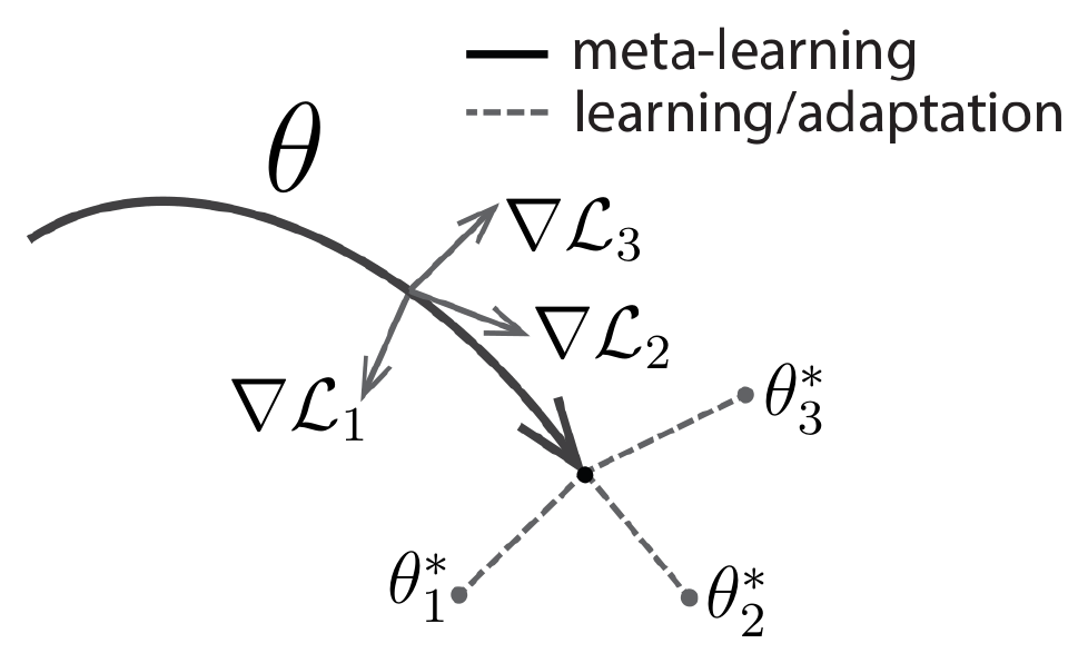
In contrast to prior work, which has sought to train recurrent neural networks that ingest entire datasets [5, 7] or feature embeddings that can be combined with nonparametric methods at test time [8, 6], we propose a method that can learn the parameters of any standard model via meta-learning in such a way as to prepare that model for fast adaptation. The intuition behind this approach is that some internal representations are more transferrable than others. For example, a neural network might learn internal features that are broadly applicable to all tasks in $p(\mathcal{T})$, rather than a single individual task. How can we encourage the emergence of such general-purpose representations? We take an explicit approach to this problem: since the model will be fine-tuned using a gradient-based learning rule on a new task, we will aim to learn a model in such a way that this gradient-based learning rule can make rapid progress on new tasks drawn from $p(\mathcal{T})$, without overfitting. In effect, we will aim to find model parameters that are sensitive to changes in the task, such that small changes in the parameters will produce large improvements on the loss function of any task drawn from $p(\mathcal{T})$, when altered in the direction of the gradient of that loss (see Figure 1). We make no assumption on the form of the model, other than to assume that it is parametrized by some parameter vector $\theta$, and that the loss function is smooth enough in $\theta$ that we can use gradient-based learning techniques.
Formally, we consider a model represented by a parametrized function $f_\theta$ with parameters $\theta$. When adapting to a new task $\mathcal{T}_i$, the model's parameters $\theta$ become $\theta_i'$. In our method, the updated parameter vector $\theta_i'$ is computed using one or more gradient descent updates on task $\mathcal{T}_i$. For example, when using one gradient update,
$ \theta_i'=\theta-\alpha \nabla_\theta \mathcal{L}_{\mathcal{T}i}(f\theta). $
The step size $\alpha$ may be fixed as a hyperparameter or meta-learned. For simplicity of notation, we will consider one gradient update for the rest of this section, but using multiple gradient updates is a straightforward extension.
The model parameters are trained by optimizing for the performance of $f_{\theta_i'}$ with respect to $\theta$ across tasks sampled from $p(\mathcal{T})$. More concretely, the meta-objective is as follows:
$ \min_\theta \sum_{\mathcal{T}i \sim p(\mathcal{T})} \mathcal{L}{\mathcal{T}i} (f{\theta_i'}) = \sum_{\mathcal{T}i \sim p(\mathcal{T})} \mathcal{L}{\mathcal{T}i} (f{\theta - \alpha \nabla_\theta \mathcal{L}_{\mathcal{T}i}(f\theta)}) $
Note that the meta-optimization is performed over the model parameters $\theta$, whereas the objective is computed using the updated model parameters $\theta'$. In effect, our proposed method aims to optimize the model parameters such that one or a small number of gradient steps on a new task will produce maximally effective behavior on that task.
The meta-optimization across tasks is performed via stochastic gradient descent (SGD), such that the model parameters $\theta$ are updated as follows:
$ \theta \leftarrow \theta - \beta \nabla_\theta \sum_{\mathcal{T}i \sim p(\mathcal{T})} \mathcal{L}{\mathcal{T}i} (f{\theta_i'})\tag{1} $
where $\beta$ is the meta step size. The full algorithm, in the general case, is outlined in Algorithm 1.
Require: $p(\mathcal{T})$: distribution over tasks
Require: $\alpha$, $\beta$: step size hyperparameters
randomly initialize $\theta$
while not done do
  Sample batch of tasks $\mathcal{T}_i \sim p(\mathcal{T})$
  for all $\mathcal{T}_i$ do
    Evaluate $\nabla_\theta \mathcal{L}_{\mathcal{T}_i}(f_\theta)$ with respect to $K$ examples
    Compute adapted parameters with gradient descent: $\theta_i'=\theta-\alpha \nabla_\theta  \mathcal{L}_{\mathcal{T}_i}(  f_\theta )$
  end for
  Update $\theta \leftarrow \theta - \beta \nabla_\theta \sum_{\mathcal{T}_i \sim p(\mathcal{T})}  \mathcal{L}_{\mathcal{T}_i} ( f_{\theta_i'})$
end while
The MAML meta-gradient update involves a gradient through a gradient. Computationally, this requires an additional backward pass through $f$ to compute Hessian-vector products, which is supported by standard deep learning libraries such as TensorFlow [9]. In our experiments, we also include a comparison to dropping this backward pass and using a first-order approximation, which we discuss in Section 5.2.
3. Species of MAML
Section Summary: The section explains how the core MAML approach can be applied to two different settings. In supervised learning, it enables models to learn new classification or regression tasks from just a handful of labeled examples by adapting parameters with standard losses such as mean-squared error or cross-entropy. In reinforcement learning, the same mechanism lets an agent quickly acquire a policy for a new task by performing a few policy-gradient updates on limited experience from that environment.
In this section, we discuss specific instantiations of our meta-learning algorithm for supervised learning and reinforcement learning. The domains differ in the form of loss function and in how data is generated by the task and presented to the model, but the same basic adaptation mechanism can be applied in both cases.
3.1 Supervised Regression and Classification
Few-shot learning is well-studied in the domain of supervised tasks, where the goal is to learn a new function from only a few input/output pairs for that task, using prior data from similar tasks for meta-learning. For example, the goal might be to classify images of a Segway after seeing only one or a few examples of a Segway, with a model that has previously seen many other types of objects. Likewise, in few-shot regression, the goal is to predict the outputs of a continuous-valued function from only a few datapoints sampled from that function, after training on many functions with similar statistical properties.
To formalize the supervised regression and classification problems in the context of the meta-learning definitions in Section 2.1, we can define the horizon $H=1$ and drop the timestep subscript on $\mathbf{x}_t$, since the model accepts a single input and produces a single output, rather than a sequence of inputs and outputs. The task $\mathcal{T}_i$ generates $K$ i.i.d. observations $\mathbf{x}$ from $q_i$, and the task loss is represented by the error between the model's output for $\mathbf{x}$ and the corresponding target values $\mathbf{y}$ for that observation and task.
Two common loss functions used for supervised classification and regression are cross-entropy and mean-squared error (MSE), which we will describe below; though, other supervised loss functions may be used as well. For regression tasks using mean-squared error, the loss takes the form:
$ \mathcal{L}{\mathcal{T}i}(f\phi) = !!!!!! \sum{\mathbf{x}^{(j)}, \mathbf{y}^{(j)} \sim \mathcal{T}i} \lVert f\phi(\mathbf{x}^{(j)}) - \mathbf{y}^{(j)} \rVert_2^2,\tag{2} $
where $\mathbf{x}^{(j)}, \mathbf{y}^{(j)}$ are an input/output pair sampled from task $\mathcal{T}_i$. In $K$-shot regression tasks, $K$ input/output pairs are provided for learning for each task.
Similarly, for discrete classification tasks with a cross-entropy loss, the loss takes the form:
$ \begin{aligned} \mathcal{L}{\mathcal{T}i}(f\phi) = !!!!!! \sum{\mathbf{x}^{(j)}, \mathbf{y}^{(j)} \sim \mathcal{T}i} !!!!!! & \mathbf{y}^{(j)} \log f\phi(\mathbf{x}^{(j)}) \ &+(1-\mathbf{y}^{(j)}) \log (1-f_\phi(\mathbf{x}^{(j)})) \end{aligned}\tag{3} $
According to the conventional terminology, $K$-shot classification tasks use $K$ input/output pairs from each class, for a total of $NK$ data points for $N$-way classification. Given a distribution over tasks $p(\mathcal{T}_i)$, these loss functions can be directly inserted into the equations in Section 2.2 to perform meta-learning, as detailed in Algorithm 2.
{REQUIRE $p(\mathcal{T})$: distribution over tasks
Require: $\alpha$, $\beta$: step size hyperparameters
randomly initialize $\theta$
while not done do
  Sample batch of tasks $\mathcal{T}_i \sim p(\mathcal{T})$
  for all $\mathcal{T}_i$ do
    Sample $K$ datapoints $\mathcal{D}=\{\mathbf{x}^{(j)}, \mathbf{y}^{(j)}\}$ from $\mathcal{T}_i$
    Evaluate $\nabla_\theta \mathcal{L}_{\mathcal{T}_i}(f_\theta)$ using $\mathcal{D}$ and $\mathcal{L}_{\mathcal{T}_i}$ in Equation (2) or (3)
    Compute adapted parameters with gradient descent: $\theta_i'=\theta-\alpha \nabla_\theta  \mathcal{L}_{\mathcal{T}_i}(  f_\theta )$
    Sample datapoints $\mathcal{D}_i'=\{\mathbf{x}^{(j)}, \mathbf{y}^{(j)}\}$ from $\mathcal{T}_i$ for the meta-update
  end for
  Update $\theta \leftarrow \theta - \beta \nabla_\theta \sum_{\mathcal{T}_i \sim p(\mathcal{T})}  \mathcal{L}_{\mathcal{T}_i} ( f_{\theta_i'})$ using each $\mathcal{D}_i'$ and $\mathcal{L}_{\mathcal{T}_i}$ in Equation 2 or 3
end while
}
3.2 Reinforcement Learning
In reinforcement learning (RL), the goal of few-shot meta-learning is to enable an agent to quickly acquire a policy for a new test task using only a small amount of experience in the test setting. A new task might involve achieving a new goal or succeeding on a previously trained goal in a new environment. For example, an agent might learn to quickly figure out how to navigate mazes so that, when faced with a new maze, it can determine how to reliably reach the exit with only a few samples. In this section, we will discuss how MAML can be applied to meta-learning for RL.
Each RL task $\mathcal{T}_i$ contains an initial state distribution $q_i(\mathbf{x}1)$ and a transition distribution $q_i(\mathbf{x}{t+1}| \mathbf{x}_t, \mathbf{a}t)$, and the loss $\mathcal{L}{\mathcal{T}i}$ corresponds to the (negative) reward function $R$. The entire task is therefore a Markov decision process (MDP) with horizon $H$, where the learner is allowed to query a limited number of sample trajectories for few-shot learning. Any aspect of the MDP may change across tasks in $p(\mathcal{T})$. The model being learned, $f\theta$, is a policy that maps from states $\mathbf{x}_t$ to a distribution over actions $\mathbf{a}_t$ at each timestep $t \in {1, ..., H}$. The loss for task $\mathcal{T}i$ and model $f\phi$ takes the form
$ \mathcal{L}{\mathcal{T}i}(f\phi) = - \mathbb{E}{\mathbf{x}t, \mathbf{a}t \sim f\phi, q{\mathcal{T}i}}\left[\sum{t=1}^H R_i(\mathbf{x}_t, \mathbf{a}_t) \right].\tag{4} $
In $K$-shot reinforcement learning, $K$ rollouts from $f_\theta$ and task $\mathcal{T}_i$, $(\mathbf{x}_1, \mathbf{a}_1, ... \mathbf{x}_H)$, and the corresponding rewards $R(\mathbf{x}t, \mathbf{a}t)$, may be used for adaptation on a new task $\mathcal{T}i$. Since the expected reward is generally not differentiable due to unknown dynamics, we use policy gradient methods to estimate the gradient both for the model gradient update(s) and the meta-optimization. Since policy gradients are an on-policy algorithm, each additional gradient step during the adaptation of $f\theta$ requires new samples from the current policy $f{\theta{i'}}$. We detail the algorithm in Algorithm 3. This algorithm has the same structure as Algorithm 2, with the principal difference being that steps 5 and 8 require sampling trajectories from the environment corresponding to task $\mathcal{T}_i$. Practical implementations of this method may also use a variety of improvements recently proposed for policy gradient algorithms, including state or action-dependent baselines and trust regions [10].
{REQUIRE $p(\mathcal{T})$: distribution over tasks
Require: $\alpha$, $\beta$: step size hyperparameters
randomly initialize $\theta$
while not done do
  Sample batch of tasks $\mathcal{T}_i \sim p(\mathcal{T})$
  for all $\mathcal{T}_i$ do
    Sample $K$ trajectories $\mathcal{D}=\{(\mathbf{x}_1, \mathbf{a}_1,... \mathbf{x}_H)\}$ using $f_\theta$ in $\mathcal{T}_i$
    Evaluate $\nabla_\theta \mathcal{L}_{\mathcal{T}_i}(f_\theta)$ using $\mathcal{D}$ and $\mathcal{L}_{\mathcal{T}_i}$ in Equation 4
    Compute adapted parameters with gradient descent: $\theta_i'=\theta-\alpha \nabla_\theta  \mathcal{L}_{\mathcal{T}_i}(  f_\theta )$
    Sample trajectories $\mathcal{D}_i'=\{(\mathbf{x}_1, \mathbf{a}_1,... \mathbf{x}_H)\}$ using $f_{\theta_i'}$ in $\mathcal{T}_i$
  end for
  Update $\theta \leftarrow \theta - \beta \nabla_\theta \sum_{\mathcal{T}_i \sim p(\mathcal{T})}  \mathcal{L}_{\mathcal{T}_i} ( f_{\theta_i'})$ using each $\mathcal{D}_i'$ and $\mathcal{L}_{\mathcal{T}_i}$ in Equation 4
end while
}
4. Related Work
Section Summary: The proposed method is a general meta-learning technique for few-shot adaptation that learns a good model initialization so standard gradient updates can quickly adjust to new tasks. It differs from other meta-learning approaches that rely on learned update rules, added parameters, recurrent memory modules, or task-specific comparison metrics, which often limit flexibility or add complexity. The approach is also distinct from standard pretraining or initialization schemes because it explicitly optimizes parameters for rapid sensitivity to new data rather than broad feature reuse.
The method that we propose in this paper addresses the general problem of meta-learning [11, 1, 12], which includes few-shot learning. A popular approach for meta-learning is to train a meta-learner that learns how to update the parameters of the learner's model [2, 13, 14]. This approach has been applied to learning to optimize deep networks [15, 3, 16], as well as for learning dynamically changing recurrent networks [17]. One recent approach learns both the weight initialization and the optimizer, for few-shot image recognition [4]. Unlike these methods, the MAML learner's weights are updated using the gradient, rather than a learned update; our method does not introduce additional parameters for meta-learning nor require a particular learner architecture.
Few-shot learning methods have also been developed for specific tasks such as generative modeling [18, 19] and image recognition [8]. One successful approach for few-shot classification is to learn to compare new examples in a learned metric space using e.g. Siamese networks [6] or recurrence with attention mechanisms [8, 20, 21]. These approaches have generated some of the most successful results, but are difficult to directly extend to other problems, such as reinforcement learning. Our method, in contrast, is agnostic to the form of the model and to the particular learning task.
Another approach to meta-learning is to train memory-augmented models on many tasks, where the recurrent learner is trained to adapt to new tasks as it is rolled out. Such networks have been applied to few-shot image recognition [5, 22] and learning "fast" reinforcement learning agents [7, 23]. Our experiments show that our method outperforms the recurrent approach on few-shot classification. Furthermore, unlike these methods, our approach simply provides a good weight initialization and uses the same gradient descent update for both the learner and meta-update. As a result, it is straightforward to finetune the learner for additional gradient steps.
Our approach is also related to methods for initialization of deep networks. In computer vision, models pretrained on large-scale image classification have been shown to learn effective features for a range of problems [24]. In contrast, our method explicitly optimizes the model for fast adaptability, allowing it to adapt to new tasks with only a few examples. Our method can also be viewed as explicitly maximizing sensitivity of new task losses to the model parameters. A number of prior works have explored sensitivity in deep networks, often in the context of initialization [25, 26]. Most of these works have considered good random initializations, though a number of papers have addressed data-dependent initializers [27, 28], including learned initializations [29, 30]. In contrast, our method explicitly trains the parameters for sensitivity on a given task distribution, allowing for extremely efficient adaptation for problems such as $K$-shot learning and rapid reinforcement learning in only one or a few gradient steps.
5. Experimental Evaluation
Section Summary: The experimental evaluation tests whether MAML can support rapid adaptation to new tasks across regression, classification, and reinforcement learning domains, while also checking if the resulting models keep improving with extra gradient steps or data. Using a simple sine-wave regression task as an initial case, the approach is compared against standard pretraining followed by fine-tuning and against an oracle that receives task identity as input. Results show that a MAML-trained model quickly fits new sine waves from only a handful of points, extrapolates sensibly outside the observed data, and continues to improve without overfitting, outperforming the baseline that cannot recover a useful representation from the same limited samples.
 {width=50%}
The goal of our experimental evaluation is to answer the following questions: (1) Can MAML enable fast learning of new tasks? (2) Can MAML be used for meta-learning in multiple different domains, including supervised regression, classification, and reinforcement learning? (3) Can a model learned with MAML continue to improve with additional gradient updates and/or examples?
All of the meta-learning problems that we consider require some amount of adaptation to new tasks at test-time. When possible, we compare our results to an oracle that receives the identity of the task (which is a problem-dependent representation) as an additional input, as an upper bound on the performance of the model. All of the experiments were performed using TensorFlow [9], which allows for automatic differentiation through the gradient update(s) during meta-learning. The code is available online[^1].
[^1]: Code for the regression and supervised experiments is at github.com/cbfinn/maml and code for the RL experiments is at github.com/cbfinn/maml_rl
5.1 Regression
We start with a simple regression problem that illustrates the basic principles of MAML. Each task involves regressing from the input to the output of a sine wave, where the amplitude and phase of the sinusoid are varied between tasks. Thus, $p(\mathcal{T})$ is continuous, where the amplitude varies within $[0.1, 5.0]$ and the phase varies within $[0, \pi]$, and the input and output both have a dimensionality of $1$. During training and testing, datapoints $\mathbf{x}$ are sampled uniformly from $[-5.0, 5.0]$. The loss is the mean-squared error between the prediction $f(\mathbf{x})$ and true value. The regressor is a neural network model with $2$ hidden layers of size $40$ with ReLU nonlinearities. When training with MAML, we use one gradient update with $K=10$ examples with a fixed step size $\alpha=0.01$, and use Adam as the meta-optimizer [31]. The baselines are likewise trained with Adam. To evaluate performance, we fine-tune a single meta-learned model on varying numbers of $K$ examples, and compare performance to two baselines: (a) pretraining on all of the tasks, which entails training a network to regress to random sinusoid functions and then, at test-time, fine-tuning with gradient descent on the $K$ provided points, using an automatically tuned step size, and (b) an oracle which receives the true amplitude and phase as input. In Appendix C, we show comparisons to additional multi-task and adaptation methods.
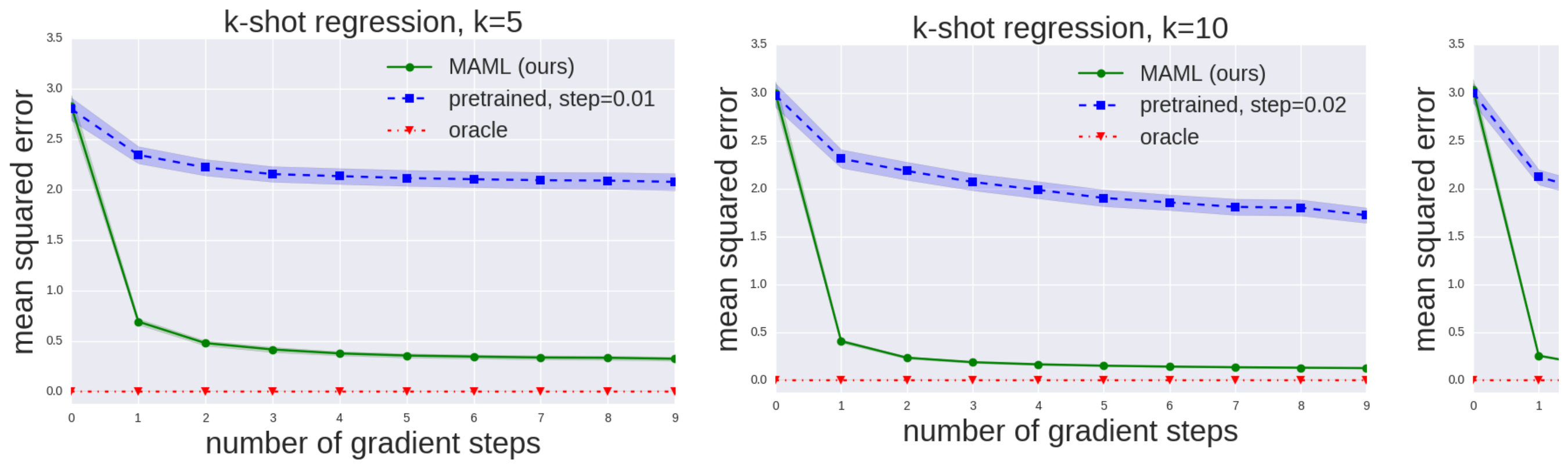
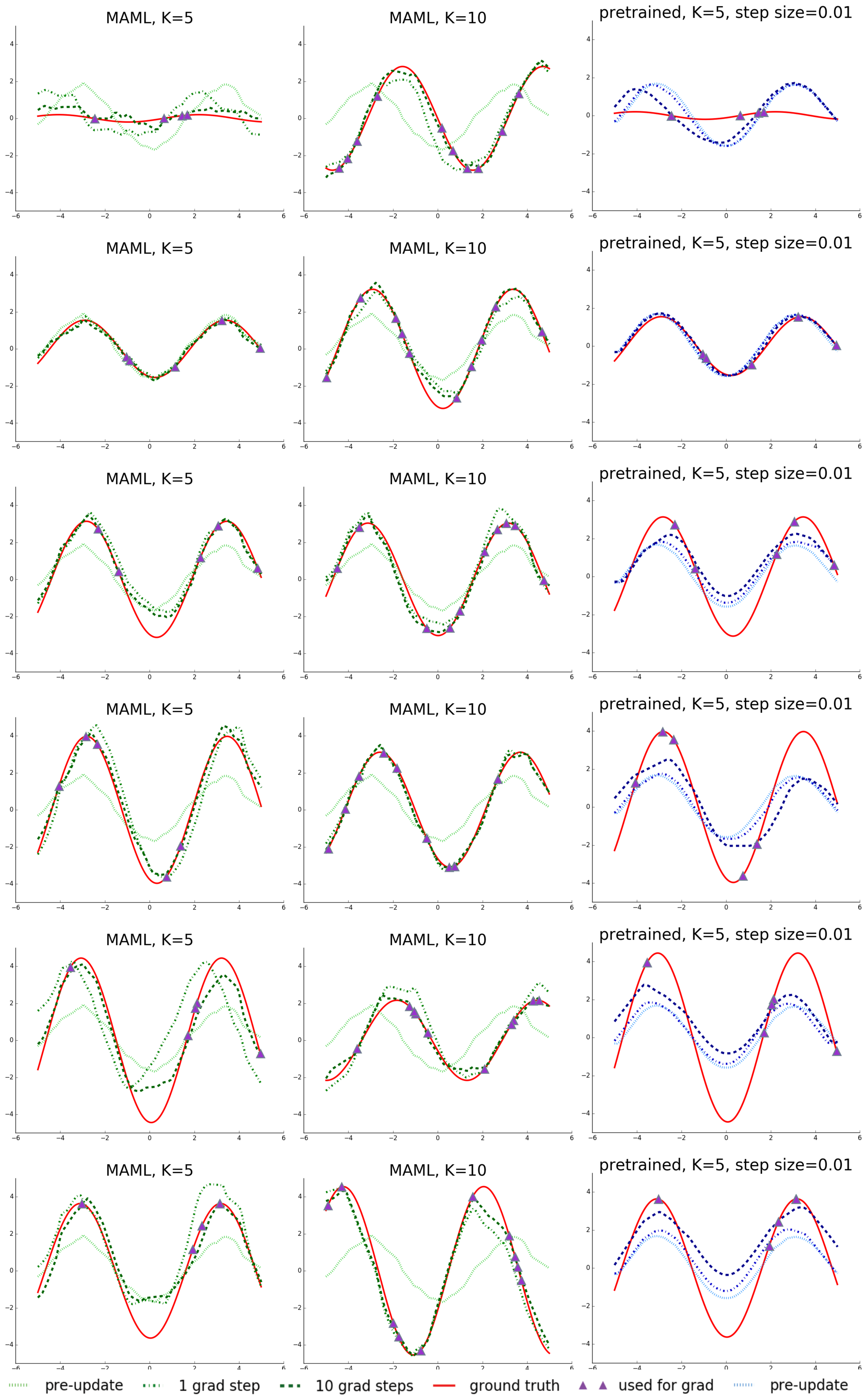
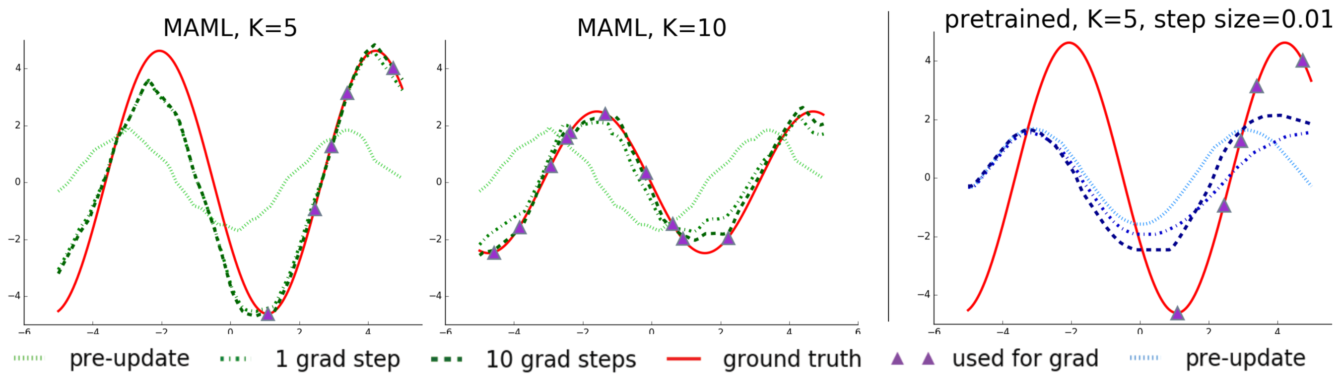
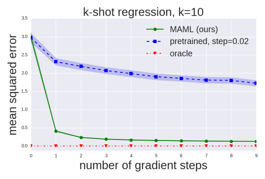
We evaluate performance by fine-tuning the model learned by MAML and the pretrained model on $K={5, 10, 20}$ datapoints. During fine-tuning, each gradient step is computed using the same $K$ datapoints. The qualitative results, shown in Figure 2 and further expanded on in Appendix B show that the learned model is able to quickly adapt with only $5$ datapoints, shown as purple triangles, whereas the model that is pretrained using standard supervised learning on all tasks is unable to adequately adapt with so few datapoints without catastrophic overfitting. Crucially, when the $K$ datapoints are all in one half of the input range, the model trained with MAML can still infer the amplitude and phase in the other half of the range, demonstrating that the MAML trained model $f$ has learned to model the periodic nature of the sine wave. Furthermore, we observe both in the qualitative and quantitative results (Figure 3 and Appendix B) that the model learned with MAML continues to improve with additional gradient steps, despite being trained for maximal performance after one gradient step. This improvement suggests that MAML optimizes the parameters such that they lie in a region that is amenable to fast adaptation and is sensitive to loss functions from $p(\mathcal{T})$, as discussed in Section 2.2, rather than overfitting to parameters $\theta$ that only improve after one step.
5.2 Classification
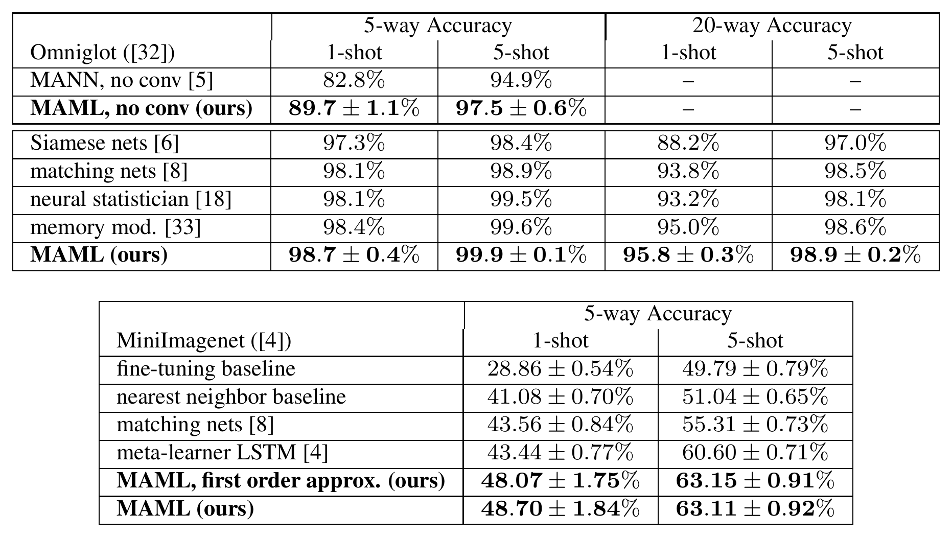
::: {caption="Table 1: Few-shot classification on held-out Omniglot characters (top) and the MiniImagenet test set (bottom). MAML achieves results that are comparable to or outperform state-of-the-art convolutional and recurrent models. Siamese nets, matching nets, and the memory module approaches are all specific to classification, and are not directly applicable to regression or RL scenarios. The ± shows 95% confidence intervals over tasks. Note that the Omniglot results may not be strictly comparable since the train/test splits used in the prior work were not available. The MiniImagenet evaluation of baseline methods and matching networks is from [4]."}
:::
To evaluate MAML in comparison to prior meta-learning and few-shot learning algorithms, we applied our method to few-shot image recognition on the Omniglot [32] and MiniImagenet datasets. The Omniglot dataset consists of 20 instances of 1623 characters from 50 different alphabets. Each instance was drawn by a different person. The MiniImagenet dataset was proposed by [4], and involves 64 training classes, 12 validation classes, and 24 test classes. The Omniglot and MiniImagenet image recognition tasks are the most common recently used few-shot learning benchmarks [8, 5, 4]. We follow the experimental protocol proposed by [8], which involves fast learning of $N$-way classification with 1 or 5 shots. The problem of $N$-way classification is set up as follows: select $N$ unseen classes, provide the model with $K$ different instances of each of the $N$ classes, and evaluate the model's ability to classify new instances within the $N$ classes. For Omniglot, we randomly select $1200$ characters for training, irrespective of alphabet, and use the remaining for testing. The Omniglot dataset is augmented with rotations by multiples of $90$ degrees, as proposed by [5].
Our model follows the same architecture as the embedding function used by [8], which has 4 modules with a $3\times3$ convolutions and $64$ filters, followed by batch normalization [34], a ReLU nonlinearity, and $2\times2$ max-pooling. The Omniglot images are downsampled to $28\times28$, so the dimensionality of the last hidden layer is $64$. As in the baseline classifier used by [8], the last layer is fed into a softmax. For Omniglot, we used strided convolutions instead of max-pooling. For MiniImagenet, we used $32$ filters per layer to reduce overfitting, as done by [4]. In order to also provide a fair comparison against memory-augmented neural networks [5] and to test the flexibility of MAML, we also provide results for a non-convolutional network. For this, we use a network with $4$ hidden layers with sizes $256$, $128$, $64$, $64$, each including batch normalization and ReLU nonlinearities, followed by a linear layer and softmax. For all models, the loss function is the cross-entropy error between the predicted and true class. Additional hyperparameter details are included in Appendix A.1.
We present the results in Table 1. The convolutional model learned by MAML compares well to the state-of-the-art results on this task, narrowly outperforming the prior methods. Some of these existing methods, such as matching networks, Siamese networks, and memory models are designed with few-shot classification in mind, and are not readily applicable to domains such as reinforcement learning. Additionally, the model learned with MAML uses fewer overall parameters compared to matching networks and the meta-learner LSTM, since the algorithm does not introduce any additional parameters beyond the weights of the classifier itself. Compared to these prior methods, memory-augmented neural networks [5] specifically, and recurrent meta-learning models in general, represent a more broadly applicable class of methods that, like MAML, can be used for other tasks such as reinforcement learning [7, 23]. However, as shown in the comparison, MAML significantly outperforms memory-augmented networks and the meta-learner LSTM on 5-way Omniglot and MiniImagenet classification, both in the $1$-shot and $5$-shot case.
A significant computational expense in MAML comes from the use of second derivatives when backpropagating the meta-gradient through the gradient operator in the meta-objective (see Equation (1)). On MiniImagenet, we show a comparison to a first-order approximation of MAML, where these second derivatives are omitted. Note that the resulting method still computes the meta-gradient at the post-update parameter values $\theta_i'$, which provides for effective meta-learning. Surprisingly however, the performance of this method is nearly the same as that obtained with full second derivatives, suggesting that most of the improvement in MAML comes from the gradients of the objective at the post-update parameter values, rather than the second order updates from differentiating through the gradient update. Past work has observed that ReLU neural networks are locally almost linear ([35]), which suggests that second derivatives may be close to zero in most cases, partially explaining the good performance of the first-order approximation. This approximation removes the need for computing Hessian-vector products in an additional backward pass, which we found led to roughly $33%$ speed-up in network computation.
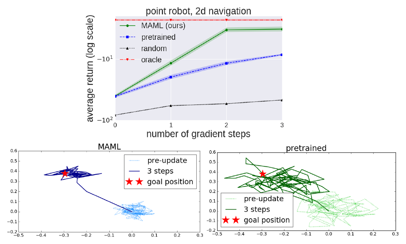
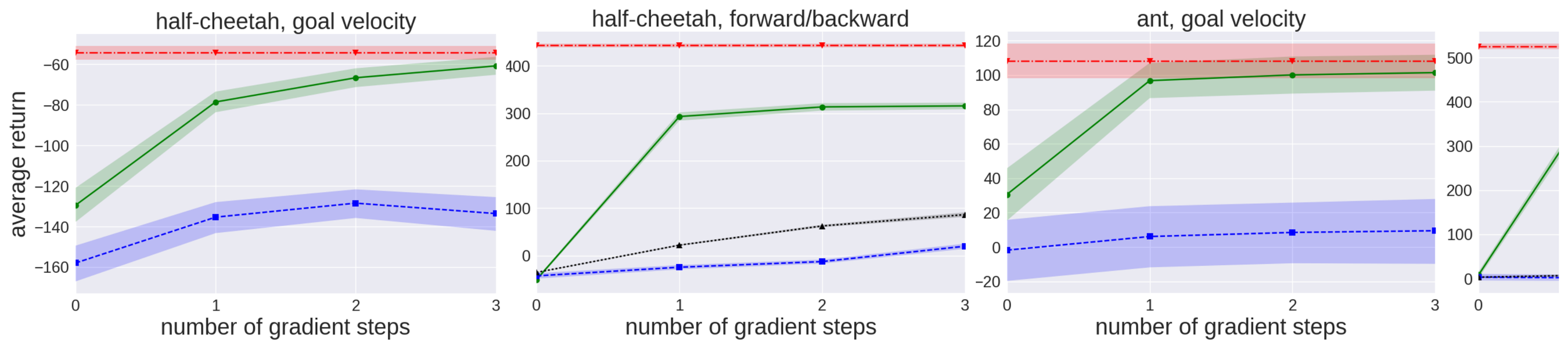
5.3 Reinforcement Learning