Fast ODE-based Sampling for Diffusion Models in Around 5 Steps

Zhenyu ZhouDefang ChenCan WangChun Chen

article2024CVPR110 citationsCVPR 2024 Highlight Paper (Top 2.8%)

Proposes AMED-Solver, a single-step ODE solver that exploits the two-dimensional subspace geometry of diffusion sampling trajectories to eliminate truncation errors and generate high-quality images in only around 5 evaluation steps.

Listen

Diffusion models have established themselves as a leading class of generative artificial intelligence, producing exceptionally high-quality and diverse images. However, their practical deployment is severely hindered by slow generation speeds, traditionally requiring hundreds to thousands of iterative computational steps. While recent mathematical techniques have reduced this requirement to under twenty steps, cutting the computational budget down to extremely few steps—such as five—causes standard numerical solvers to suffer severe approximation errors and sharp drops in image quality. Alternative distillation-based techniques can achieve rapid generation but demand massive re-training expenses and alter model behavior.

The article aims to develop and evaluate a new sampling approach that maintains high image generation quality under extreme computational constraints of around five function evaluations, without requiring costly model retraining.

To achieve this, the authors observed an underlying geometric property of diffusion sampling trajectories: despite existing in image spaces with thousands of dimensions, the generation paths consistently lie almost entirely within a simple two-dimensional plane. Leveraging this insight, the authors created the Approximate Mean-Direction Solver (AMED-Solver) and a generalized plugin extension (AMED-Plugin). The approach trains a tiny auxiliary neural network using knowledge distillation from pre-generated sample paths. This network learns to predict optimal intermediate time steps and scaling factors, allowing the solver to directly navigate along the true mean direction of the trajectory rather than relying on heuristic approximations. The authors evaluated the framework across benchmark datasets spanning image resolutions from 32x32 to 512x512 pixels, including CIFAR-10, ImageNet, FFHQ, LSUN Bedroom, and Stable Diffusion.

The findings show that the proposed approach delivers substantial performance gains in ultra-fast sampling regimes. First, when operating at only 5 function evaluations, the method achieved state-of-the-art image quality among numerical solver methods across multiple benchmarks, reaching Fréchet Inception Distance scores of 6.61 on CIFAR-10, 10.74 on ImageNet 64x64, and 13.20 on LSUN Bedroom. Second, applying the plugin to existing multi-step solvers significantly improved baseline outputs, reducing error scores by roughly 30% to 50% in low-step settings. Third, the lightweight predictor network introduces virtually no sampling overhead and requires negligible training resources—taking as little as a few minutes to a few hours on a single standard graphics processing unit.

These results demonstrate that organizations deploying diffusion models can achieve near-instantaneous image generation while reducing inference compute costs and hardware requirements. Unlike full-model distillation, this approach preserves the core mathematical formulation of the underlying model, ensuring stability and compatibility with existing workflows.

Organizations operating or deploying diffusion models in production should consider integrating this plug-and-play solver framework to lower generation latency and hosting expenses. The authors note, however, that solver performance remains sensitive to the underlying scheduling of time steps, indicating that time-schedule tuning is necessary to maximize image fidelity across different model architectures and data domains.

The State Key Laboratory of Blockchain and Data Security Zhejiang University diffusion probabilistic models ode diffusion models ODE-based sampling fast ODE solvers

arXiv: 2312.00094

Paper: DPM-Solver: A Fast ODE Solver for Diffusion Probabilistic Model Sampling in Around 10 Steps, Cheng Lu et al. (2022). It introduces DPM-Solver, the foundational fast ODE numerical solver whose semi-linear formulation and multi-step approximation errors in ultra-low step counts directly motivate AMED's mean-direction approach.
Paper: Denoising Diffusion Implicit Models, Jiaming Song et al. (2021). It establishes deterministic, non-Markovian sampling for diffusion models, framing generative inference as an ODE trajectory that subsequent fast ODE solvers optimize.
Paper: Elucidating the Design Space of Diffusion-Based Generative Models, Tero Karras et al. (2022). It systematizes diffusion ODE formulations, noise schedules, and high-order deterministic numerical integrators that serve as standard baselines for fast sampling.
Paper: Score-Based Generative Modeling through Stochastic Differential Equations, Yang Song et al. (2021). It introduces the continuous probability flow ODE formulation that enables deterministic ODE-based trajectory sampling in diffusion models.
Paper: Progressive Distillation for Fast Sampling of Diffusion Models, Tim Salimans et al. (2022). It establishes few-step generation through progressive distillation, providing the primary retraining-heavy baseline that the retraining-free AMED solver aims to improve upon.
Paper: Consistency Models, Yang Song et al. (2023). It defines consistency distillation along diffusion ODE trajectories, representing the benchmark standard for few-step sampling against which numerical solvers are compared.
Paper: High-Resolution Image Synthesis with Latent Diffusion Models, Robin Rombach et al. (2022). It provides the latent diffusion architecture and pre-trained Stable Diffusion models on which fast ODE sampling plug-ins and evaluations are executed.
Paper: Denoising Diffusion Probabilistic Models, Jonathan Ho et al. (2020). It introduces the core denoising diffusion probabilistic modeling paradigm upon which all subsequent ODE trajectory formulations and acceleration solvers depend.

Paper: Mean Flows for One-step Generative Modeling, Zhengyang Geng et al. (2025). It extends the concept of learning average velocities across trajectory intervals to achieve direct one-step generative flow modeling.
Paper: Variational Flow Maps: Make Some Noise for One-Step Conditional Generation, Abbas Mammadov et al. (2026). It applies few-step and one-step generative flow principles to solve downstream conditional inverse problems.
Paper: Generative Modeling via Drifting, Mingyang Deng et al. (2026). It develops an alternative paradigm to multi-step ODE integration by training models via drifting fields to accomplish one-step generation.

Cover for Fast ODE-based Sampling for Diffusion Models in Around 5 Steps

Abstract

Sampling from diffusion models can be treated as solving the corresponding ordinary differential equations (ODEs), with the aim of obtaining an accurate solution with as few number of function evaluations (NFE) as possible. Recently, various fast samplers utilizing higher-order ODE solvers have emerged and achieved better performance than the initial first-order one. However, these numerical methods inherently result in certain approximation errors, which significantly degrades sample quality with extremely small NFE (e.g., around 5). In contrast, based on the geometric observation that each sampling trajectory almost lies in a two-dimensional subspace embedded in the ambient space, we propose Approximate MEan-Direction Solver (AMED-Solver) that eliminates truncation errors by directly learning the mean direction for fast diffusion sampling. Besides, our method can be easily used as a plugin to further improve existing ODE-based samplers. Extensive experiments on image synthesis with the resolution ranging from 32 to 512 demonstrate the effectiveness of our method. With only 5 NFE, we achieve 6.61 FID on CIFAR-10, 10.74 FID on ImageNet 64x64, and 13.20 FID on LSUN Bedroom. Our code is available at https://github.com/zju-pi/diff-sampler.

Topics

diffusion probabilistic models ode

Keywords

diffusion models ODE-based sampling fast ODE solvers Approximate MEan-Direction Solver probability flow ODE single-step ODE solvers discretization error stochastic differential equations

1. Introduction
2. Background
2.1. Diffusion Models
2.2. Categorization of Previous Fast ODE Solvers
3. Our Proposed AMED-Solver
3.1. The Sampling Trajectory Almost Lies in a Two-Dimensional Subspace
3.2. Approximate Mean-Direction Solver
3.3. AMED as A Plugin
3.4. Training and Sampling
3.5. Comparing with Distillation-based Methods
4. Experiments
4.1. Settings
4.2. Image Generation
4.3. Ablation Study
5. Conclusion
6. Acknowledgement
References

Knowls

Knowl 1 — Approximate mean-direction update
model/method
For the EDM parameterization used in the paper, the probability-flow ODE is written as $d x_t=\boldsymbol{\epsilon}_\theta(x_t,t)\,dt$ , where $x_t\in\mathbb{R}^d$ is the diffusion state at noise level $t>0$ and $\boldsymbol{\epsilon}_\theta:\mathbb{R}^d\times\mathbb{R}_{>0}\to\mathbb{R}^d$ is the pretrained noise-prediction network. Sampling uses a decreasing time step from $t_{n+1}$ to $t_n$ , with $t_n<t_{n+1}$ .

AMED-Solver chooses an intermediate time $s_n\in(t_n,t_{n+1})$ and a scalar direction factor $c_n\in\mathbb{R}$ so that the network direction at $(x_{s_n},s_n)$ approximates the average ODE direction over the whole interval:
$\boldsymbol{\epsilon}_\theta(x_{s_n},s_n)\approx \frac{c_n}{t_n-t_{n+1}}\int_{t_{n+1}}^{t_n}\boldsymbol{\epsilon}_\theta(x_t,t)\,dt.$
The resulting single-step update is
$x_{t_n}\approx x_{t_{n+1}}+c_n(t_n-t_{n+1})\boldsymbol{\epsilon}_\theta(x_{s_n},s_n).$
The intermediate state $x_{s_n}$ is obtained by an intermediate solver step. The standard DPM-Solver-2 update is recovered when $s_n=\sqrt{t_nt_{n+1}}$ and $c_n=1$ ; AMED instead learns both quantities for each sampling state, reducing the truncation error caused by a fixed numerical approximation.
Knowl 2 — Two-dimensional geometry of diffusion sampling trajectories
empirical result
The paper empirically finds that a complete diffusion sampling trajectory is nearly contained in a two-dimensional subspace, despite the image state having thousands or hundreds of thousands of dimensions. PCA was applied to 1,000 trajectories generated with the EDM solver using 80 NFE on CIFAR-10 $32\times32$ , FFHQ $64\times64$ , ImageNet $64\times64$ , and LSUN Bedroom $256\times256$ .

For each state $x_t$ , the projection $\widetilde{x}_t$ onto the top two principal components was evaluated using the relative error $\lVert x_t-\widetilde{x}_t\rVert_2/\lVert x_t\rVert_2$ . The averaged relative projection error stayed at a small level and did not exceed $8\%$ across the tested datasets, while the cumulative variance plots on page 4 show that the top two components explain nearly all trajectory variance. The ambient dimensions are $3\cdot32^2=3072$ , $3\cdot64^2=12288$ , and $3\cdot256^2=196608$ . This observation motivates approximating the vector-valued integral in the ODE update by a learned mean direction.
Knowl 3 — AMED predictor and distillation objective
model/method
The learned AMED predictor $g_\phi$ receives the current U-Net bottleneck feature $h_{t_{n+1}}$ and the two endpoint times, and predicts the intermediate location and direction scale:
$\{s_n,c_n\}=g_\phi(h_{t_{n+1}},t_{n+1},t_n).$
In the implemented parameterization, the network predicts $r_n$ and $c_n$ , then converts the interpolation coefficient $r_n$ into a geometric intermediate time,
$s_n=t_n^{r_n}t_{n+1}^{1-r_n}.$
The predictor channel-wise mean-pools the U-Net bottleneck, processes the result through fully connected layers, concatenates the time embedding, and applies another fully connected layer with a sigmoid output. Its purpose is to predict two scalar sampling parameters rather than a high-dimensional image state.

Training uses knowledge distillation from a more accurate teacher trajectory. If $\Phi_s$ denotes the student solver, $x_{t_{n+1}}$ is the student state, and $y_{t_n}$ is the teacher state at the same scheduled time, the loss for interval $n$ is
$\mathcal{L}_{t_n}(\phi)=d\!\left(\Phi_s\!\left(x_{t_{n+1}},t_{n+1},t_n,\{s_n,c_n\}\right),y_{t_n}\right),$
where $d$ is a distance between states; the experiments use the $L_2$ distance. Teacher trajectories insert $M$ intermediate points between each pair of student times. For a polynomial schedule with exponent $\rho$ , the teacher points are
$s_n^i=\left(t_n^{1/\rho}+\frac{i}{M+1}\left(t_{n+1}^{1/\rho}-t_n^{1/\rho}\right)\right)^\rho,\qquad i=1,\ldots,M.$
The predictor is trained progressively from the highest-noise interval toward the data endpoint, applying $N-1$ backpropagations per training loop.
Knowl 4 — AMED sampling procedure
algorithm
AMED sampling takes a trained predictor $g_\phi$ , a decreasing sampling schedule $t_N>\cdots>t_1$ , and either the AMED-Solver or a baseline ODE solver. It returns a generated state at $t_1$ .
Input: Trained predictor $g_\phi$ , time schedule $t_1<\cdots<t_N$ , pretrained noise network $\boldsymbol{\epsilon}_\theta$ , and ODE solver.
Sample $x_{t_N}\sim\mathcal{N}(0,t_N^2I)$ .
for $n=N-1$ down to $1$ do
    Evaluate the U-Net at $(x_{t_{n+1}},t_{n+1})$ and extract bottleneck feature $h_{t_{n+1}}$ .
    Predict $(r_n,c_n)=g_\phi(h_{t_{n+1}},t_{n+1},t_n)$ .
    Set $s_n=t_n^{r_n}t_{n+1}^{1-r_n}$ .
    For AMED-Solver, take an Euler intermediate step
         $x_{s_n}=x_{t_{n+1}}+(s_n-t_{n+1})\boldsymbol{\epsilon}_\theta(x_{t_{n+1}},t_{n+1})$ .
    Update to $t_n$ using
         $x_{t_n}=x_{t_{n+1}}+c_n(t_n-t_{n+1})\boldsymbol{\epsilon}_\theta(x_{s_n},s_n)$ .
    For AMED-Plugin, replace the last two operations by the corresponding baseline solver's two substeps and scale the direction in the latter substep by $c_n$ .
end for
Output: Generated sample $x_{t_1}$ .
Without the analytical first step, each interval requires two U-Net evaluations, giving $2(N-1)$ NFE. The predictor itself adds negligible sampling computation because it has only about 9,000 parameters.
Knowl 5 — AMED-Plugin generalizes learned direction selection to existing solvers
model/method
AMED-Plugin applies the same learned intermediate-time and scaling-factor idea to an arbitrary fast ODE solver. For a baseline solver represented by $\Phi$ , let $\Lambda_n=\{s_n,c_n\}$ denote the parameters used on the interval from $t_{n+1}$ to $t_n$ . The plugin performs the baseline solver's intermediate evaluation at the predicted $s_n$ rather than at a fixed heuristic time, and multiplies the direction used in the latter part of the step by the predicted $c_n$ .

The fixed DPM-Solver-2 choice uses $s_n=\sqrt{t_nt_{n+1}}$ and $c_n=1$ . AMED-Plugin learns both quantities from the current U-Net bottleneck feature, allowing the direction to adapt to the current trajectory and to the solver being improved. In the grid-search validation reported on page 5, the schedule used $\epsilon=0.002$ , $T=80$ , and $N=6$ ; a Heun teacher with 80 NFE supplied the reference trajectory. Searching the intermediate coefficient $r_n$ produced a trajectory closer to the reference than the fixed geometric-mean baseline in most intervals, supporting the use of learned rather than fixed intermediate locations.
Knowl 6 — Analytical first step and optional time rescaling
model/method
At the initial high-noise state $x_{t_N}$ , the paper observes that the predicted direction $\boldsymbol{\epsilon}_\theta(x_{t_N},t_N)$ is nearly aligned with $x_{t_N}$ . The analytical first step (AFS) therefore uses $x_{t_N}$ itself as the first-step direction, eliminating one U-Net evaluation. AFS is reported to cause little degradation, and sometimes improves quality, on the small-resolution datasets tested.

For AMED-Plugin applied to DDIM, iPNDM, and DPM-Solver++ on $32\times32$ and $64\times64$ datasets, the predictor can optionally learn an additional positive time-scaling factor $a_n$ . The intermediate evaluation for the second substep then uses $\boldsymbol{\epsilon}_\theta(x_{s_n},a_ns_n)$ instead of $\boldsymbol{\epsilon}_\theta(x_{s_n},s_n)$ . This expands the available solution family and improved some of the reported small-resolution results. With AFS, the otherwise even evaluation count $2(N-1)$ becomes odd, enabling the experiments at 3, 5, 7, and 9 NFE.
Knowl 7 — Experimental configuration for fast-sampling evaluation
experimental setup
AMED-Solver and AMED-Plugin were evaluated on CIFAR-10 $32\times32$ , FFHQ $64\times64$ , ImageNet $64\times64$ , LSUN Bedroom $256\times256$ , and Stable Diffusion at $512$ resolution. The models were pretrained pixel-space diffusion models or the latent-space Stable Diffusion model. Baselines included DDIM, DPM-Solver-2, third-order DPM-Solver++, UniPC, and fourth-order improved PNDM (iPNDM).

The main schedule was the polynomial schedule with $\rho=7$ ; DPM-Solver++ and UniPC used their recommended logSNR schedules, while AMED-Solver used a uniform schedule on CIFAR-10, FFHQ, and ImageNet. The AMED predictor was trained using 10,000 images, took 2--8 minutes on CIFAR-10 and 1--3 hours on LSUN Bedroom on one NVIDIA A100, and used about 9,000 parameters. DPM-Solver-2 or EDM with doubled NFE supplied AMED-Solver teachers; AMED-Plugin used the same solver as the student, with $M=1$ for DPM-Solver-2 and $M=2$ for other solvers. Image quality was measured by FID on 50,000 generated images, except for Stable Diffusion, where FID used 30,000 images generated from 30,000 fixed MS-COCO validation prompts.
Knowl 8 — Image-generation results around five NFE
data/table
The FID results reported on page 7 compare solver-based samplers at 3, 5, 7, and 9 NFE; lower is better. AMED-Solver consistently improves over the other single-step solvers, while AMED-Plugin often reaches or surpasses the multi-step baselines. The entries are:
Could not parse LaTeX table
The dagger marks runs that additionally learned the time-scaling factors $a_n$ . At 5 NFE, the strongest reported values are FID 6.61 on CIFAR-10, 10.74 on ImageNet, and 13.20 on LSUN Bedroom for AMED-Plugin or AMED-Solver configurations.
Knowl 9 — Stable Diffusion acceleration with AMED-Plugin
empirical result
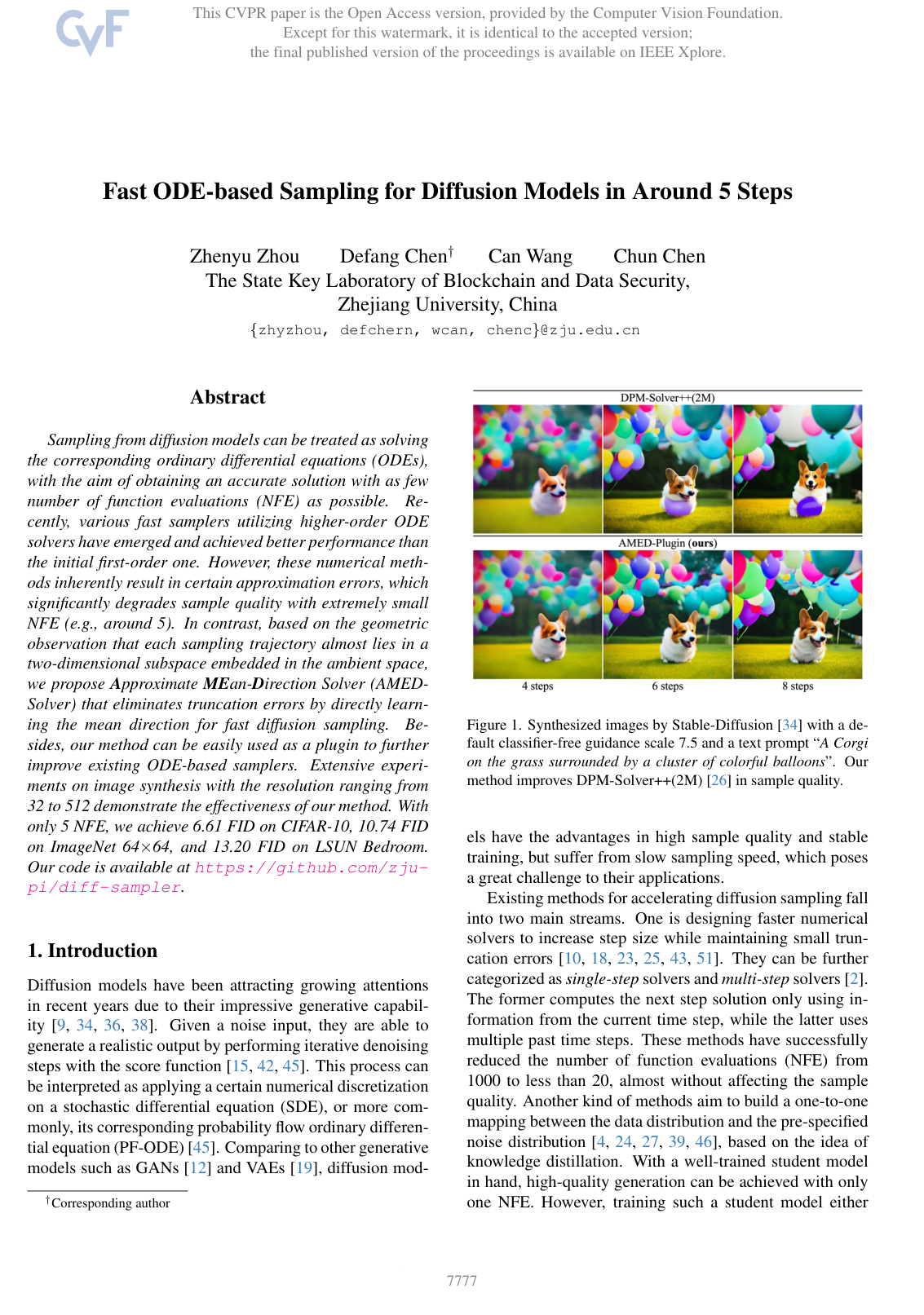
On Stable Diffusion v1.4 at $512$ resolution with classifier-free guidance scale 7.5, AMED-Plugin was applied to DPM-Solver++(2M). The evaluation used 30,000 fixed text prompts sampled from the MS-COCO validation set, and one solver step required two U-Net evaluations. The FID values reported on page 7 were:
Could not parse LaTeX table
AMED-Plugin improves the baseline at every tested evaluation budget, including the extremely small budget of 8 NFE.
Knowl 10 — Teacher and schedule ablations
empirical result
The ablations on CIFAR-10 show that the quality of the AMED predictor depends on how closely the teacher solver matches the student solver. At 3, 5, 7, and 9 NFE, AMED-Solver trained with DPM-Solver++(3M), iPNDM, DPM-Solver-2, and EDM teachers obtained FIDs of $(35.68,12.34,11.28,9.65)$ , $(32.38,12.42,10.09,8.54)$ , $(18.49,11.60,11.64,9.23)$ , and $(28.99,7.59,4.36,3.67)$ , respectively. For AMED-Plugin on iPNDM, the corresponding values were $(16.00,7.57,4.28,2.85)$ , $(10.81,6.61,3.65,2.63)$ , $(12.07,8.19,4.52,2.66)$ , and $(29.62,10.58,9.36,4.44)$ . The best results generally came from a teacher whose sampling procedure resembled the student procedure.

The schedule ablation used DPM-Solver++(3M) on CIFAR-10. The baseline FIDs for uniform, polynomial, and logSNR schedules were $(76.80,26.90,16.80,13.44)$ , $(70.04,31.66,11.30,6.45)$ , and $(110.0,24.97,6.74,3.42)$ at 3, 5, 7, and 9 NFE. Applying AMED-Plugin changed them to $(33.61,13.24,8.89,8.24)$ , $(32.47,19.59,9.60,4.39)$ , and $(25.95,7.68,4.51,3.03)$ , respectively. Thus the plugin improves all tested schedules, even though the preferred fixed schedule depends on the solver, dataset, and NFE budget.
Knowl 11 — Limitation: fixed schedules remain sensitive at very low NFE
limitation
Fast diffusion ODE solvers remain highly sensitive to the chosen time schedule when the NFE budget is small. The paper reports that no single fixed schedule performs well in all tested situations. AMED-Plugin can adaptively adjust intermediate times and therefore partly alleviates this problem, but it does not eliminate the dependence on the underlying schedule. The authors leave the design of schedules informed directly by the geometric shape of sampling trajectories as future work.

Coverage note — The paper's qualitative Stable Diffusion image comparisons and its discussion contrasting AMED with full distillation methods were not made separate knowls because the quantitative Stable Diffusion result is included and the comparison is contextual rather than an additional contributed method.

References

1.Brian DO Anderson. Reverse-time diffusion equation models. Stochastic Processes and their Applications, 12(3):313–326, 1982.
2.Kendall Atkinson, Weimin Han, and David E Stewart. Numerical solution of ordinary differential equations. John Wiley & Sons, 2011.
3.Fan Bao, Chongxuan Li, Jun Zhu, and Bo Zhang. Analytic-dpm: an analytic estimate of the optimal reverse variance in diffusion probabilistic models. arXiv preprint arXiv:2201.06503, 2022.
4.David Berthelot, Arnaud Autef, Jierui Lin, Dian Ang Yap, Shuangfei Zhai, Siyuan Hu, Daniel Zheng, Walter Talbot, and Eric Gu. Tract: Denoising diffusion models with transitive closure time-distillation. arXiv preprint arXiv:2303.04248, 2023.
5.Mikołaj Binkowski, Danica J Sutherland, Michael Arbel, and Arthur Gretton. Demystifying mmd gans. arXiv preprint arXiv:1801.01401, 2018.
6.Defang Chen, Zhenyu Zhou, Jian-Ping Mei, Chunhua Shen, Chun Chen, and Can Wang. A geometric perspective on diffusion models. arXiv preprint arXiv:2305.19947, 2023.
7.Elliott Ward Cheney, EW Cheney, and W Cheney. Analysis for applied mathematics. Springer, 2001.
8.Giannis Daras, Yuval Dagan, Alexandros G Dimakis, and Constantinos Daskalakis. Consistent diffusion models: Mitigating sampling drift by learning to be consistent. arXiv preprint arXiv:2302.09057, 2023.
9.Prafulla Dhariwal and Alex Nichol. Diffusion models beat gans on image synthesis. In Advances in Neural Information Processing Systems, 2021.
10.Tim Dockhorn, Arash Vahdat, and Karsten Kreis. Genie: Higher-order denoising diffusion solvers. In Advances in Neural Information Processing Systems, 2022.
11.William Feller. On the theory of stochastic processes, with particular reference to applications. In Proceedings of the First Berkeley Symposium on Mathematical Statistics and Probability, pages 403–432, 1949.
12.Ian Goodfellow, Jean Pouget-Abadie, Mehdi Mirza, Bing Xu, David Warde-Farley, Sherjil Ozair, Aaron Courville, and Yoshua Bengio. Generative adversarial nets. Advances in neural information processing systems, 27, 2014.
13.Jiatao Gu, Shuangfei Zhai, Yizhe Zhang, Lingjie Liu, and Josh Susskind. Boot: Data-free distillation of denoising diffusion models with bootstrapping. arXiv preprint arXiv:2306.05544, 2023.
14.Martin Heusel, Hubert Ramsauer, Thomas Unterthiner, Bernhard Nessler, and Sepp Hochreiter. GANs trained by a two time-scale update rule converge to a local Nash equilibrium. In Advances in Neural Information Processing Systems, pages 6626–6637, 2017.
15.Jonathan Ho, Ajay Jain, and Pieter Abbeel. Denoising diffusion probabilistic models. In Advances in Neural Information Processing Systems, 2020.
16.Aapo Hyvarinen. Estimation of non-normalized statistical models by score matching. Journal of Machine Learning Research, 6:695–709, 2005.
17.Tero Karras, Samuli Laine, and Timo Aila. A style-based generator architecture for generative adversarial networks. In Proceedings of the IEEE/CVF conference on computer vision and pattern recognition, pages 4401–4410, 2019.
18.Tero Karras, Miika Aittala, Timo Aila, and Samuli Laine. Elucidating the design space of diffusion-based generative models. In Advances in Neural Information Processing Systems, 2022.
19.Diederik P Kingma and Max Welling. Auto-encoding variational bayes. arXiv preprint arXiv:1312.6114, 2013.
20.Diederik P Kingma, Tim Salimans, Ben Poole, and Jonathan Ho. Variational diffusion models. In Advances in Neural Information Processing Systems, 2021.
21.Alex Krizhevsky and Geoffrey Hinton. Learning multiple layers of features from tiny images. Technical Report, 2009.
22.Tsung-Yi Lin, Michael Maire, Serge Belongie, James Hays, Pietro Perona, Deva Ramanan, Piotr Dollar, and C Lawrence Zitnick. Microsoft coco: Common objects in context. In Computer Vision–ECCV 2014: 13th European Conference, Zurich, Switzerland, September 6-12, 2014, Proceedings, Part V 13, pages 740–755. Springer, 2014.
23.Luping Liu, Yi Ren, Zhijie Lin, and Zhou Zhao. Pseudo numerical methods for diffusion models on manifolds. In International Conference on Learning Representations, 2022.
24.Xingchao Liu, Chengyue Gong, and Qiang Liu. Flow straight and fast: Learning to generate and transfer data with rectified flow. arXiv preprint arXiv:2209.03003, 2022.
25.Cheng Lu, Yuhao Zhou, Fan Bao, Jianfei Chen, Chongxuan Li, and Jun Zhu. Dpm-solver: A fast ode solver for diffusion probabilistic model sampling in around 10 steps. In Advances in Neural Information Processing Systems, 2022.
26.Cheng Lu, Yuhao Zhou, Fan Bao, Jianfei Chen, Chongxuan Li, and Jun Zhu. Dpm-solver++: Fast solver for guided sampling of diffusion probabilistic models. arXiv preprint arXiv:2211.01095, 2022.
27.Eric Luhman and Troy Luhman. Knowledge distillation in iterative generative models for improved sampling speed. arXiv preprint arXiv:2101.02388, 2021.
28.Siwei Lyu. Interpretation and generalization of score matching. In Proceedings of the Twenty-Fifth Conference on Uncertainty in Artificial Intelligence, pages 359–366, 2009.
29.Dimitra Maoutsa, Sebastian Reich, and Manfred Opper. Interacting particle solutions of fokker–planck equations through gradient–log–density estimation. arXiv preprint arXiv:2006.00702, 2020.
30.Alexander Quinn Nichol and Prafulla Dhariwal. Improved denoising diffusion probabilistic models. In International Conference on Machine Learning, pages 8162–8171. PMLR, 2021.
31.Bernt Oksendal. Stochastic differential equations: an introduction with applications. Springer Science & Business Media, 2013.
32.Eckhard Platen and Nicola Bruti-Liberati. Numerical solution of stochastic differential equations with jumps in finance. Springer Science & Business Media, 2010.
33.Aditya Ramesh, Mikhail Pavlov, Gabriel Goh, Scott Gray, Chelsea Voss, Alec Radford, Mark Chen, and Ilya Sutskever. Zero-shot text-to-image generation. In International conference on machine learning, pages 8821–8831. Pmlr, 2021.
34.Robin Rombach, Andreas Blattmann, Dominik Lorenz, Patrick Esser, and Bjorn Ommer. High-resolution image synthesis with latent diffusion models. In Proceedings of the IEEE/CVF Conference on Computer Vision and Pattern Recognition, pages 10684–10695, 2022.
35.Olaf Ronneberger, Philipp Fischer, and Thomas Brox. U-net: Convolutional networks for biomedical image segmentation. In Medical Image Computing and Computer-Assisted Intervention–MICCAI 2015: 18th International Conference, Munich, Germany, October 5-9, 2015, Proceedings, Part III 18, pages 234–241. Springer, 2015.
36.Nataniel Ruiz, Yuanzhen Li, Varun Jampani, Yael Pritch, Michael Rubinstein, and Kfir Aberman. Dreambooth: Fine tuning text-to-image diffusion models for subject-driven generation. In Proceedings of the IEEE/CVF Conference on Computer Vision and Pattern Recognition, pages 22500–22510, 2023.
37.Olga Russakovsky, Jia Deng, Hao Su, Jonathan Krause, Sanjeev Satheesh, Sean Ma, Zhiheng Huang, Andrej Karpathy, Aditya Khosla, Michael S. Bernstein, Alexander C. Berg, and Fei-Fei Li. Imagenet large scale visual recognition challenge. International Journal of Computer Vision, 115(3):211–252, 2015.
38.Chitwan Saharia, William Chan, Saurabh Saxena, Lala Li, Jay Whang, Emily L Denton, Kamyar Ghasemipour, Raphael Gontijo Lopes, Burcu Karagol Ayan, Tim Salimans, et al. Photorealistic text-to-image diffusion models with deep language understanding. In Advances in Neural Information Processing Systems, pages 36479–36494, 2022.
39.Tim Salimans and Jonathan Ho. Progressive distillation for fast sampling of diffusion models. In International Conference on Learning Representations, 2022.
40.Antoine Salmona, Valentin De Bortoli, Julie Delon, and Agnes Desolneux. Can push-forward generative models fit multimodal distributions? Advances in Neural Information Processing Systems, 35:10766–10779, 2022.
41.Simo Sarkkӓ and Arno Solin. Applied stochastic differential equations. Cambridge University Press, 2019.
42.Jascha Sohl-Dickstein, Eric Weiss, Niru Maheswaranathan, and Surya Ganguli. Deep unsupervised learning using nonequilibrium thermodynamics. In International conference on machine learning, pages 2256–2265. PMLR, 2015.
43.Jiaming Song, Chenlin Meng, and Stefano Ermon. Denoising diffusion implicit models. In International Conference on Learning Representations, 2021.
44.Yang Song and Stefano Ermon. Generative modeling by estimating gradients of the data distribution. In Advances in Neural Information Processing Systems, 2019.
45.Yang Song, Jascha Sohl-Dickstein, Diederik P. Kingma, Abhishek Kumar, Stefano Ermon, and Ben Poole. Score-based generative modeling through stochastic differential equations. In International Conference on Learning Representations, 2021.
46.Yang Song, Prafulla Dhariwal, Mark Chen, and Ilya Sutskever. Consistency models. In International Conference on Machine learning, 2023.
47.Roman Vershynin. High-dimensional probability: An introduction with applications in data science. Cambridge university press, 2018.
48.Daniel Watson, William Chan, Jonathan Ho, and Mohammad Norouzi. Learning fast samplers for diffusion models by differentiating through sample quality. In International Conference on Learning Representations, 2021.
49.Mengfei Xia, Yujun Shen, Changsong Lei, Yu Zhou, Ran Yi, Deli Zhao, Wenping Wang, and Yong-jin Liu. Towards more accurate diffusion model acceleration with a timestep aligner. arXiv preprint arXiv:2310.09469, 2023.
50.Fisher Yu, Ari Seff, Yinda Zhang, Shuran Song, Thomas Funkhouser, and Jianxiong Xiao. Lsun: Construction of a large-scale image dataset using deep learning with humans in the loop. arXiv preprint arXiv:1506.03365, 2015.
51.Qinsheng Zhang and Yongxin Chen. Fast sampling of diffusion models with exponential integrator. In International Conference on Learning Representations, 2023.
52.Wenliang Zhao, Lujia Bai, Yongming Rao, Jie Zhou, and Jiwen Lu. Unipc: A unified predictor-corrector framework for fast sampling of diffusion models. arXiv preprint arXiv:2302.04867, 2023.

Citation

MLA

Zhou, Z., et al. “Fast ODE-based Sampling for Diffusion Models in Around 5 Steps”. arXiv, 2023, http://arxiv.org/abs/2312.00094v3.

APA

Zhou, Z., Chen, D., Wang, C., & Chen, C. (2023). Fast ODE-based Sampling for Diffusion Models in Around 5 Steps. arXiv. http://arxiv.org/abs/2312.00094v3

Chicago

Zhou, Z., D. Chen, C. Wang, and C. Chen. 2023. “Fast ODE-based Sampling for Diffusion Models in Around 5 Steps”. arXiv. http://arxiv.org/abs/2312.00094v3.

Harvard

Zhou, Z. et al. (2023) “Fast ODE-based Sampling for Diffusion Models in Around 5 Steps”, arXiv [Preprint]. Available at: http://arxiv.org/abs/2312.00094v3.

Vancouver

1. Zhou Z, Chen D, Wang C, Chen C (2023) Fast ODE-based Sampling for Diffusion Models in Around 5 Steps. arXiv

BibTeX

@article{zhou2023fast,
  title = {Fast ODE-based Sampling for Diffusion Models in Around 5 Steps},
  author = {Zhou, Zhenyu and Chen, Defang and Wang, Can and Chen, Chun},
  year = {2023},
  journal = {arXiv},
  url = {http://arxiv.org/abs/2312.00094v3},
  eprint = {2312.00094}
}

Metadata:arXiv

Access the Paper

This paper is available from its original source. Click below to access the PDF.

Open PDF

License: IEEE

Fast ODE-based Sampling for Diffusion Models in Around 5 Steps

Abstract

Topics

Keywords

Table of Contents

Knowls

Knowl 1 — Approximate mean-direction update

Knowl 2 — Two-dimensional geometry of diffusion sampling trajectories

Knowl 3 — AMED predictor and distillation objective

Knowl 4 — AMED sampling procedure

Knowl 5 — AMED-Plugin generalizes learned direction selection to existing solvers

Knowl 6 — Analytical first step and optional time rescaling

Knowl 7 — Experimental configuration for fast-sampling evaluation

Knowl 8 — Image-generation results around five NFE

Knowl 9 — Stable Diffusion acceleration with AMED-Plugin

Knowl 10 — Teacher and schedule ablations

Knowl 11 — Limitation: fixed schedules remain sensitive at very low NFE

References

Citation

BibTeX

Access the Paper